Which is Better for Individual Participant Data Meta-Analysis of Zero-Inflated Count Outcomes, One-Step or Two-Step Analysis? A Simulation Study

Abstract

Meta-analysis using individual participant data (IPD) is an important methodology in intervention research because it (a) increases accuracy and precision of estimates, (b) allows researchers to investigate mediators and moderators of treatment effects, and (c) makes use of extant data. IPD meta-analysis can be conducted either via a one-step approach that uses data from all studies simultaneously, or a two-step approach, which aggregates data for each study and then combines them in a traditional meta-analysis model. Unfortunately, there are no evidence-based guidelines for how best to approach IPD meta-analysis for count outcomes with many zeroes, such as alcohol use. We used simulation to compare the performance of four hurdle models (3 one-step and 1 two-step models) for zero-inflated count IPD, under realistic data conditions. Overall, all models yielded adequate coverage and bias for the treatment effect in the count portion of the model, across all data conditions. However, in the zero portion, the treatment effect was underestimated in most models and data conditions, especially when there were fewer studies. The performance of both one- and two-step approaches depended on the formulation of the treatment effects, suggesting a need to carefully consider model assumptions and specifications when using IPD.

Keywords:

• Monte Carlo simulation
• integrative data analysis
• IDA
• zero-altered count variables
• overall intervention effect
• overall treatment effect
• complex research synthesis

Introduction

Meta-analysis using individual participant data (IPD) is an important methodology in intervention research because it (a) increases accuracy and precision of estimates, (b) allows for the examination of covariates without potential ecological inference bias (Debray et al., 2015), and (c) leverages extant data. In particular, the meta-analysis of IPD affords greater flexibility than traditional, aggregate data meta-analysis to account for differences in participants, intervention approaches, study designs, and outcome measures across studies. IPD meta-analysis and aggregate data meta-analysis often produce comparable results when considering the average effect across multiple studies, such as an overall treatment effect size (Tierney et al., 2020). However, IPD meta-analysis is preferable to aggregate data meta-analysis as the use of participant-level data allows for a consistent statistical model across all studies as well as the ability to more flexibly tailor the model to a variety of outcome types, such as dichotomous (i.e., binary event) or count outcome variables. Thus, the analysis of IPD better ensures that the overall findings are based on a consistent set of statistical assumptions. Hence, IPD meta-analysis has long been considered the “gold standard” in meta-analysis (Sutton & Higgins, 2008).

The best practices for IPD meta-analyses with count outcomes are an area of ongoing research with a lack of guidance based on rigorous empirical data (e.g., simulation study). Count outcomes are commonly encountered in social behavioral research, with outcome examples including alcohol use quantity, number of sexual risk behaviors, and number of suicide-related behaviors. The Poisson and negative binomial (NB) models and their derivatives are commonly used for such outcomes. One assumption of the Poisson model is that the variability (i.e., dispersion) of the outcome is equal to the mean. The NB model extends the Poisson by incorporating a dispersion parameter, which can accommodate situations where the variability of the outcome is higher than the mean (i.e., overdispersion). In addition, count outcomes often exhibit a greater frequency of zero outcomes than would be expected by either the Poisson or NB models. Ignoring zero inflation in the outcome (called “zero-inflation bias”; Zhou et al., 2021) could lead to biased results and subsequently incorrect inference (Perumean-Chaney et al., 2013), although biased estimates may be corrected mathematically in some situations using summary-level data (see Zhou et al., 2021). Outcomes with excessive zeroes can be accommodated by modeling the outcome in two parts: (1) the probability of zero drinking and (2) the number of drinks when drinking is non-zero. Count outcomes where zero responses are kept separate from the non-zero portion of the distribution are known as hurdle models (Atkins et al., 2013; Atkins & Gallop, 2007). Hurdle models can be implemented in Mplus (Muthén & Muthén, 1998-2022) and R (R Core Team, 2022) and have been used in recent applied research (e.g., Huh et al., 2015, 2019; Wood et al., 2010).

An alternative to the hurdle model is a zero-inflated model, a type of mixture model that distinguishes between two types of zeroes: (a) zero counts, which would correspond with drinkers who happened not to drink during the period of interest, and (b) “excess zeroes” beyond what would be predicted by an ordinary count distribution, which would correspond with alcohol abstainers who never drink. Despite the theoretical difference in how they consider zeroes, hurdle models and zero-inflated models produce highly similar estimates in practice (Atkins et al., 2013). Thus, this article focuses on the hurdle model approach due to its simpler interpretation with respect to zeroes.

Hurdle NB models can be applied to IPD meta-analysis to accommodate count outcomes with excessive zeroes and over-dispersion using either a one-step or two-step meta-analysis approach (Simmonds et al., 2005, 2011). In a “one-step” or “one-stage” approach, participant-level data from different studies are examined simultaneously in a single model. Using a single model allows researchers to explicitly address the data structure, such as clustering within studies and participant-level missing data. Furthermore, the one-step IPD meta-analysis methods use a more exact likelihood specification compared to the two-step methods. For example, individual-level moderators and mediators of treatment effects can be directly modeled in a one-step analysis, but not in a two-step analysis. However, one-step IPD meta-analysis methods can be computationally intensive and challenging to implement (Burke et al., 2017). A second approach to IPD meta-analysis, which has been the most common (Simmonds et al., 2015), is a “two-step” or “two-stage” approach in which participant-level data are first aggregated to the study level (e.g., study-specific estimates of the treatment effect). These study-level data are then combined using traditional meta-analytic methods to estimate the overall effect and between-study heterogeneity.

In the context of count outcomes, different sample populations can produce markedly different outcome distributions (see Mun et al., 2022), which has implications with respect to the choice of a one- or two-step analysis. For example, when an alcohol intervention study focuses on a broad population of individuals, the outcome distribution may have a disproportionate frequency of zeroes due to the presence of alcohol abstainers and occasional nondrinkers. In contrast, studies of higher-risk individuals, such as heavy drinkers, may have outcome distributions consisting of mostly non-zero responses with very few zero responses (i.e., zero drinks). When one or more studies have few or no zero responses, a two-step approach using hurdle models in the first step of meta-analysis may be difficult or impossible because those studies will not produce a treatment effect with respect to zero drinking that can be combined in the second-step analysis. One-step models using multilevel modeling have greater flexibility to accommodate treatment effects that are missing by design, which we detail in the “One-step IPD Meta-analysis” section. In contrast, there can be data situations where a two-step meta-analysis may provide flexibility, for example, when underlying distributions differ by study (see Mun et al., 2022).

Although the advantages of a one-step approach over a two-step approach are clear in principle, it is not clear empirically when the two approaches produce the same answer (Kontopantelis, 2018) and under what circumstances the two approaches will diverge (Burke et al., 2017). The few studies that have examined this question suggest that one- and two-step approaches provide a similar answer when focused on the overall effect (i.e., treatment effects) for continuous outcomes (Kontopantelis, 2018; Lin & Zeng, 2010; Mathew & Nordström, 2010) or binary outcomes (Cheng et al., 2019; Debray et al., 2012; Lin & Zeng, 2010; Stewart et al., 2012). Chen et al. (2020) demonstrated via numerical studies and actual data analysis that both continuous and binary outcomes obtained from summary statistics can be as efficient as IPD. However, they also noted a loss of efficiency (6–20%) with a two-step approach when sample size was not sufficient. To the best of our knowledge, no studies have evaluated the relative performance of one- vs. two-step IPD meta-analysis approaches for count data with excess zeroes.

If one- and two-step IPD approaches generate comparable results, a two-step approach to IPD meta-analysis may have an important advantage over a one-step approach because estimating the overall effect does not require raw data. Aggregate data can be derived for each study by the original investigators, which can be shared for the second-step synthesis. Although it is increasingly common to share IPD, data availability remains a barrier to IPD meta-analysis. If aggregate data derived under a common model can be combined in the second-step meta-analysis without bias or loss of power, compared with one-step IPD meta-analysis, two-step IPD meta-analysis can be counted on when data availability may be limited. However, if one- vs. two-step IPD meta-analysis approaches have different statistical performance outcomes, it is also important to know under which data conditions different results emerge.

The current study was also motivated by the practical constraints encountered in one-step IPD meta-analysis. IPD from multiple independent trials tend to come from heterogeneous study designs, which produce an unbalanced design when pooled, resulting in estimation challenges (Huh et al., 2019). The fact that IPD can be analyzed in multiple ways within the one-step IPD meta-analysis approach, compared to the two-step IPD meta-analysis approach, also raises an open question of whether meta-analysis outcomes are sensitive to different modeling assumptions. The present study addresses this gap in the literature by comparing the performance of four different modeling strategies for one-step and two-step IPD meta-analysis in the context of count data with varying degrees of excess zeroes. More specifically, we compare the bias and coverage of the intervention estimates from one- and two-step IPD meta-analysis approaches using the multilevel hurdle NB model via a Monte Carlo simulation under realistic conditions when synthesizing data across behavioral intervention studies.

IPD meta-analysis models for count data with excess zeroes

This section introduces four statistical models for IPD meta-analysis for count data with excess zeroes. The two most common modeling approaches for count data with excess zeroes are zero-inflated count models (i.e., zero-inflated Poisson or zero-inflated NB) and hurdle models, which are both two-part approaches consisting of a binary logistic and a count regression sub-model. An advantage of hurdle models compared to zero-inflated models is that they are easier to interpret and estimate because of the clear distinction between zeroes and non-zero counts. In the current study, the four models for IPD meta-analysis are based on hurdle models in which the outcome is modeled in two parts: (a) a logistic regression examining the likelihood of a zero outcome vs. a non-zero outcome and (b) a zero-truncated count regression examining the mean parameter for non-zero count outcomes.

One-step IPD meta-analysis

We first detail three approaches for one-step IPD meta-analysis in which the study-specific treatment effects and the overall effect of treatment across studies are estimated in a single, simultaneous analysis. Model 1 is a conventional, multilevel model in which study is defined at the highest level (i.e., cluster) of the model and one or more dummy-coded predictor variables for treatment assignment predicting intervention outcome, the effect of which can vary by study. Model 1 is ideal when studies are preplanned with the same design, such as having the same number of study arms (e.g., all two-arm trials). Model 2 is a reformulation of Model 1 that excludes the fixed effect for treatment and accommodates differences in the number of treatment groups (see Huh et al., 2015, 2019) by (1) using unique randomized groups at the highest level of the multilevel model (MLM), instead of study, and (2) estimating treatment effects by computing the posterior distribution of the difference between each treatment group and its corresponding control group within studies. Finally, Model 3 is an extension of Model 2 that includes an additional fixed effect for treatment. Later in the “Simulation Design” section, Model 1 will serve as the data generating model and the gold standard against which three other models will be compared, assuming a balanced number of treatment arms (i.e., two) across studies.

Model 1: MLM with study at the highest level and study-specific treatment effects

A conventional strategy for estimating treatment effects across multiple studies is via a two- or three-level MLM, where study is defined at the highest level of the model and participants are nested within studies. If the data are structured such that each participant is associated with a single observation (e.g., one follow-up assessment per participant), a two-level model may be sufficient where participants (level 1) are nested within study (level 2). However, if the data consist of multiple follow-up observations nested within participant, a three-level model is a logical choice, where repeated observations (level 1) are nested within participant (level 2), and participants are nested within study (level 3). To derive study-specific treatment effects as well as an overall estimate of treatment effect, a varying intercept coefficient can be defined for each study in combination with a varying treatment slope (for a two-arm design) to account for variation in the treatment effect across studies.

When modeling a count outcome with excess zeroes, such as drinking quantity, a multilevel hurdle model can be conducted that treats the outcome as a mixture of two parts: (1) the probability of no drinks vs. any drinks, which can be modeled via logistic regression, and (2) the number of drinks when drinking is non-zero, which can be modeled using a zero-truncated count regression, such as the Poisson or NB models. For the present study, we consider the zero-truncated NB model, which includes an additional overdispersion parameter to accommodate situations where the variance of drinking, when it is non-zero, is greater than would be predicted by the Poisson model. This situation, where the variance of a variable is greater than its mean, is relatively common in studies with alcohol outcomes data and, more broadly, in behavioral intervention and prevention studies.

The logistic portion of the hurdle model (Equation (1a)) examines whether an individual participant from a specific study did not drink at a particular assessment point. Here, the subscript (B) identifies regression coefficients from the logistic sub-model, and I is an indicator function whose value is equal to one if the condition inside the parentheses is true and zero otherwise. Let $\mathrm{Pr}\left[{\mathrm{DRINKS}}_{t>0,is}=0\right]$ be the probability of individual i in study s not drinking at assessment t, and $\mathrm{Pr}\left[{\mathrm{DRINKS}}_{t>0,is}\ge 1\right]$ be the probability of individual i in study s drinking one or more drinks at assessment t. (1a) $$\begin{array}{ll}\text{log}\left(\frac{\text{Pr}\left[{\text{DRINKS}}_{t>0,is}=0\right]}{\text{Pr}\left[{\text{DRINKS}}_{t>0,is}\ge 1\right]}\right)& =b_{0\left(B\right)}+b_{1\left(B\right)}{\text{TREATMENT}}_{is}\\ +b_{2\left(B\right)}I\left({\text{DRINKS}}_{t=0,is}=0\right)+\hspace{0.17em}{b}_{3\left(B\right)}{\text{DRINKS}}_{t=0,is}\\ +u_{0s\left(B\right)}+u_{1s\left(B\right)}{\text{TREATMENT}}_{is}+r_{0i\left(B\right)}\end{array}$$(1a)

Let $\mathrm{E}\left[\left.{\mathrm{DRINKS}}_{t>0,is}\right|{\mathrm{DRINKS}}_{t>0,is}\ge 1\right]$ be the expected number of drinks, when drinking, which was one or greater for individual i in study s at assessment t in Equation (1b). To constrain predictions to positive counts greater than or equal to one, the outcome is modeled as the natural logarithm of the expected number of drinks (i.e., log link function) as follows: (1b) $$\begin{array}{c}\begin{array}{cc}\hspace{0.17em}\log \hspace{0.17em}\left(\mathrm{E}\left[\left.{\mathrm{DRINKS}}_{t>0,is}\right|{\mathrm{DRINKS}}_{t>0,is}\ge 1\right]\right)=& b_{0\left(C\right)}+b_{1\left(C\right)}{\mathrm{TREATMENT}}_{is}+\\ & {\hspace{0.17em}b}_{2\left(C\right)}I\left({\mathrm{DRINKS}}_{t=0,is}=0\right)+b_{3\left(C\right)}{\mathrm{DRINKS}}_{t=0,is}+\\ & {\hspace{0.17em}u}_{0s\left(C\right)}+u_{1s\left(C\right)}{\mathrm{TREATMENT}}_{is}+r_{0i\left(C\right)}\end{array}\end{array},$$(1b) where (C) identifies regression coefficients from the zero-truncated NB sub-model.

The nonvarying regression coefficients $b_{1\left(B\right)}$ and $b_{1\left(C\right)}$ quantify the covariate-adjusted average difference in post-baseline drinking between participants who received treatment compared to control participants. Covariates for baseline drinking are incorporated into both the logistic (Equation (1a)) and zero-truncated NB (Equation (1b)) models to adjust for baseline drinking. Baseline drinking, ${\text{DRINKS}}_{t=0,is},$ was divided into two related covariates to account for: (1) no drinking vs. any drinking and (2) the number of drinks at baseline including zeroes. These two covariates are the third and fourth terms on the right-hand side of Equations (1a and 1b). Consequently, individuals who did not drink at baseline have non-zero $b_{2\left(B\right)}$ and $b_{2\left(C\right)}$ terms (i.e., the association between not drinking vs. drinking at baseline and postbaseline drinking), while $b_{3\left(B\right)}$ and $b_{3\left(C\right)}$ are zeroed out in Equations (1a and 1b), respectively, because they are multiplied by zero when the number of baseline drinks is equal to zero. However, individuals who drank at baseline are represented by non-zero $b_{3\left(B\right)}$ and $b_{3\left(C\right)}$ terms, while b_2(B) and b_2(C) are zeroed out in Equations (1a and 1b) when the number of baseline drinks is non-zero.

Model 1 is a logical formulation of an MLM for one-step IPD meta-analysis. However, its disadvantages include greater complexity involving study-specific random intercepts and treatment slopes, which may lead to greater nonconvergence during estimation. Specifically, nonconvergence in estimation may be more likely when extending the model to include three-arm or four-arm trials where most studies are two-arm trials (e.g., a treatment group and a control group). In such situations, any study with just two groups will have missing data for the third and fourth intervention groups, when all of these studies are synthesized together. In addition, with more than one treatment type, it is likely that not all combinations of treatments would have been “directly” evaluated “head to head” in all studies. This results in rank deficiency because of insufficient study-level data to estimate the variance-covariance matrices of the study-specific random coefficients (i.e., for $u_{0s\left(B\right)},$ $u_{1s\left(B\right)};$ and $u_{0s\left(C\right)},$ $u_{1s\left(C\right)}$) (see Huh et al., 2019 for a detailed explanation).

In summary, Model 1 is ideal if there is no study-level missing data in treatment groups. However, when analyzing IPD from studies with different treatment arms, the estimation difficulties of Model 1 under this common data situation point to the need for alternative modeling strategies. The next approach, which was first implemented by Huh et al. (2015), is a simpler alternative to Model 1 in that it only uses a varying intercept to model treatment effects, and circumvents the challenge described above when treatment arms across studies are unbalanced and not directly estimable.

Model 2: MLM with study-by-treatment combinations at the highest level

To accommodate “missing” study-by-treatment combinations, a single varying intercept parameter representing unique study-by-treatment combinations can be specified, as detailed by Huh et al. (2019), each of which represents a unique randomized group. Model 2 is a one-step MLM with a random intercept for a unique study-by-treatment arm combination, where the treatment effects are calculated as postestimation contrasts of the random intercept between groups within studies. Model 2 can be implemented using a Bayesian approach to produce a full joint posterior distribution for the random effects (i.e., study-by-treatment effects), which makes computing the posterior distribution of the difference between each treatment group and its corresponding control group straightforward (see “Estimation Considerations” later).

The multilevel hurdle NB model that incorporates a varying intercept coefficient for unique randomized groups (i.e., study-by-treatment arm combinations) can be seen in Equations (2a and 2b). The logistic portion of the hurdle model (Equation (2a)) estimates whether an individual participant belonging to a specific randomized group did not drink (at a particular assessment point). Let $\mathrm{Pr}\left[{\mathrm{DRINKS}}_{t>0,ig}=0\right]$ be the probability of individual i in randomized group g not drinking at assessment t, and $\mathrm{Pr}\left[{\mathrm{DRINKS}}_{t>0,ig}\ge 1\right]$ be the probability of individual i in randomized group g drinking one or more drinks at assessment t. The randomized groups identified by the subscript g represent the active treatment and control comparison groups across all studies. For example, five two-arm studies, each with one treatment arm and one control arm, would translate to a total of 10 randomized groups. To constrain predictions to range from 0 to 1, the outcome is modeled as the natural logarithm of the odds (i.e., logit link function) of the probability of not drinking vs. any drinking, as follows: (2a) $$\begin{array}{c}\begin{array}{cc}\mathrm{l}\mathrm{og}\left(\frac{\mathrm{Pr}\left[{\mathrm{DRINKS}}_{t>0,ig}=0\right]}{\mathrm{Pr}\left[{\mathrm{DRINKS}}_{t>0,ig}\ge 1\right]}\right)=& b_{0\left(B\right)}+b_{1\left(B\right)}I\left({\mathrm{DRINKS}}_{t=0,ig}=0\right)+\\ & {\hspace{0.17em}b}_{2\left(B\right)}{\mathrm{DRINKS}}_{t=0,ig}+\\ & u_{0g\left(B\right)}+r_{0i\left(B\right)}\end{array}\end{array},$$(2a) where (B) identifies regression coefficients from the logistic model. The zero-truncated NB portion of the hurdle model (Equation (2b)) models occasions where drinking did occur, for individual i in randomized group g at assessment t, as follows: (2b) $$\begin{array}{c}\begin{array}{cc}\hspace{0.17em}\log \hspace{0.17em}\left(\mathrm{E}\left[\left.{\mathrm{DRINKS}}_{t>0,ig}\right|{\mathrm{DRINKS}}_{t>0,ig}\ge 1\right]\right)=& b_{0\left(C\right)}+b_{1\left(C\right)}I\left({\mathrm{DRINKS}}_{t=0,ig}=0\right)+\hspace{0.17em}\\ & b_{2\left(C\right)}\left({\mathrm{DRINKS}}_{t=0,ig}\right)+\\ & u_{0g\left(C\right)}+r_{0i\left(C\right)}\end{array}\end{array},$$(2b) where (C) identifies regression coefficients from the zero-truncated NB model. To control for baseline drinking, the covariates, $I({\mathrm{DRINKS}}_{t=0,ig}=0)$ and ${\mathrm{DRINKS}}_{t=0,ig},$ are included in Equations (2a and 2b), as in Model 1. Similarly, the nonvarying regression coefficients associated with the covariates for baseline drinking quantify the effect of (1) not drinking vs. drinking ($b_{1\left(B\right)},$ $b_{1\left(C\right)}$), and (2) the number of drinks when drinking ($b_{2\left(B\right)},$ $b_{2\left(C\right)}$), on the average drinking outcome across all randomized groups.

The group-level varying coefficients $u_{0g\left(B\right)}$ and $u_{0g\left(C\right)}$ in the logistic and zero-truncated NB sub-models, respectively, quantify the extent to which each randomized group (i.e., control or intervention group across studies) differs from the covariate-adjusted average drinking outcome across all groups.

Model 3: An extension of model 2 with an additional fixed treatment effect

Model 3 is a modification of Model 2 that incorporates a fixed effect for treatment arm, such that the overall treatment effect is directly estimated as a parameter, rather than indirectly derived as post estimation contrasts within studies from the varying intercept terms (i.e., random intercepts) of the unique randomized groups as in Model 2. The multilevel hurdle NB model that incorporates a fixed effect for treatment in combination with varying intercept coefficients for unique randomized groups (i.e., study-by-treatment arm combinations) is described in Equations (3a and 3b). (3a) $$\begin{array}{c}\begin{array}{cc}\mathrm{l}\mathrm{og}\left(\frac{\mathrm{Pr}\left[{\mathrm{DRINKS}}_{t>0,ig}=0\right]}{\mathrm{Pr}\left[{\mathrm{DRINKS}}_{t>0,ig}\ge 1\right]}\right)=& b_{0\left(B\right)}+b_{1\left(B\right)}{\mathrm{TREATMENT}}_{ig}+\\ & {\hspace{0.17em}b}_{2\left(B\right)}I\left({\mathrm{DRINKS}}_{t=0,ig}=0\right)+b_{3\left(B\right)}{\mathrm{DRINKS}}_{t=0,ig}+\\ & {\hspace{0.17em}u}_{0g\left(B\right)}+r_{0i\left(B\right)}, \mathrm{and}\end{array}\end{array}$$(3a) (3b) $$\begin{array}{c}\begin{array}{cc}\hspace{0.17em}\log \hspace{0.17em}\left(\mathrm{E}\left[\left.{\mathrm{DRINKS}}_{t>0,ig}\right|{\mathrm{DRINKS}}_{t>0,ig}\ge 1\right]\right)=& b_{0\left(C\right)}+b_{1\left(C\right)}{\mathrm{TREATMENT}}_{ig}+\\ & b_{2\left(C\right)}I\left({\mathrm{DRINKS}}_{t=0,ig}=0\right)+\hspace{0.17em}{b}_{3\left(C\right)}{\mathrm{DRINKS}}_{t=0,ig}+\\ & u_{0g\left(C\right)}+r_{0i\left(C\right)}\end{array}\end{array},$$(3b) where the subscripts have the same interpretation as Equations (2a and 2b). The nonvarying treatment coefficients $b_{1\left(B\right)}$ and $b_{1\left(C\right)}$ in the logistic and zero-truncated NB models, respectively, quantify the average covariate-adjusted difference in the average drinking outcome across groups for participants randomized to a treatment group (i.e., ${\mathrm{TREATMENT}}_{ig}$ = 1) vs. a control group.

In Model 3, the group-level varying coefficients $u_{0g\left(B\right)}$ and $u_{0g\left(C\right)}$ quantify the extent to which each randomized group differs from the (1) treatment- and (2) covariate-adjusted average drinking outcome. Thus, when a randomized group corresponds with a control condition (i.e., ${\mathrm{TREATMENT}}_{ig}$ = 0), $u_{0g\left(B\right)}$ and $u_{0g\left(C\right)}$ quantify the extent to which that specific control group differs from the average covariate-adjusted drinking outcome across all control participants. Similarly, when a randomized group corresponds with an intervention condition, $u_{0g\left(B\right)}$ and $u_{0g\left(C\right)}$ quantify the extent to which a specific intervention group differs from the average covariate-adjusted drinking outcome in the intervention group.

Two-step IPD meta-analysis

Next, we describe a two-step IPD meta-analysis approach to a hurdle model. A two-step approach may be computationally more straightforward for larger-scale IPD meta-analyses involving a larger sample of studies (e.g., 20 or more) or a larger number of covariates, especially when using zero-altered count models, which can be more computationally demanding to estimate using a one-step approach. Also, because the second step of a two-step IPD meta-analysis is functionally equivalent to a conventional meta-analysis, this approach may be useful as a means of incorporating aggregate data in a meta-analysis that were identically analyzed (e.g., zero-inflated Poisson) by the original investigators. The application of a hurdle model in the first step of the IPD meta-analysis produces two sets of treatment effect estimates, which can be synthesized in the second step using a bivariate meta-analysis, where each study contributes two outcomes, corresponding to the treatment effect in the logistic and zero-truncated portions of the hurdle model.

Model 4: Two-step bivariate random-effects meta-analysis

In the first-step analysis, a multilevel hurdle NB is estimated for each study (Equations (4a and 4b)) to simultaneously derive a study-specific treatment effect on (a) the probability of zero drinking, and (b) the quantity of drinking when non-zero. The first step of the analysis produces (a) a log odds ratio and (b) a log rate ratio for each study, corresponding to the logistic and zero-truncated NB portions of the hurdle model, respectively. (4a) $$\begin{array}{c}\begin{array}{cc}\mathrm{l}\mathrm{og}\left(\frac{\mathrm{Pr}\left[{\mathrm{DRINKS}}_{t>0,i}=0\right]}{\mathrm{Pr}\left[{\mathrm{DRINKS}}_{t>0,i}\ge 1\right]}\right)=& b_{0\left(B\right)}+b_{1\left(B\right)}{\mathrm{TREATMENT}}_i+\hspace{0.17em}\\ & b_{2\left(B\right)}I\left({\mathrm{DRINKS}}_{t=0,i}=0\right)+b_{3\left(B\right)}{\mathrm{DRINKS}}_{t=0,i}+\hspace{0.17em}{r}_{0i\left(B\right)}, \text{and}\end{array}\\ & \end{array}$$(4a) (4b) $$\begin{array}{c}\begin{array}{cc}\hspace{0.17em}\log \hspace{0.17em}\left(\mathrm{E}\left[{\mathrm{DRINKS}}_{ti}\right]{\mathrm{DRINKS}}_{ti}\ge 1\right)=& b_{0\left(C\right)}+b_{1\left(C\right)}{\mathrm{TREATMENT}}_i+\hspace{0.17em}\\ & b_{2\left(B\right)}I\left({\mathrm{DRINKS}}_{t=0,i}=0\right)+b_{3\left(B\right)}{\mathrm{DRINKS}}_{t=0,i}+\hspace{0.17em}{r}_{0i\left(C\right)}\end{array}\\ & \end{array}.$$(4b)

All subscripts are previously defined. Note that there are no subscripts g or s in Equations (4a) or (4b) to indicate that the model is estimated separately. The first-step analysis in Equations (4a and 4b) is repeated separately and sequentially for each study, and the study-specific treatment effects and corresponding variance estimates are subsequently extracted and carried forward to the second-step analysis.

In the second-step analysis, the study-specific treatment effect estimates are collated as a vector of covariate-adjusted treatment effect estimates ($b_{1s\left(B\right)}$ and $b_{1s\left(C\right)},$ where s indexes the study) and evaluated in a bivariate random-effects meta-analysis model (Equation (4c)) to estimate a pooled, overall treatment effect. We note that it is possible to combine the entire set of coefficients (i.e., also including $b_{0s\left(B\right)},$ $b_{2s\left(B\right)},$ $b_{3s\left(B\right)},$ $b_{0s\left(C\right)},$ $b_{2s\left(C\right)},$ and $b_{3s\left(C\right)}$). However, this is challenging to estimate and rarely done in practice. Thus, we opted for a bivariate meta-analysis model that focuses on only the treatment effects for simplicity. Hence, subscript 1 can be dropped. We kept subscript 1 in Equation (4c) to identify the two vectors of point estimates for study-specific treatment effects from the first-step analysis but dropped it from the population parameters in Equations (4c and 4d). Equation (4c) for level-1 study-specific population parameters and Equation (4d) for level-2 hyperparameters can be shown as follows: (4c) $$\begin{array}{c}\left[\begin{array}{c}{b}_{1s\left(B\right)}\\ b_{1s\left(C\right)}\end{array}\right]\sim N\left(\left[\begin{array}{c}{\theta }_{s\left(B\right)}\\ {\theta }_{s\left(C\right)}\end{array}\right], \left[\begin{array}{cc}{\sigma }_{s\left(B\right)}^2& {\rho }_{\left(B,C\right)}{\sigma }_{s\left(B\right)}{\sigma }_{s\left(C\right)}\\ {\rho }_{\left(B,C\right)}{\sigma }_{s\left(B\right)}{\sigma }_{s\left(C\right)}& {\sigma }_{s\left(C\right)}^2\end{array}\right]\right)\end{array},\begin{array}{c}\text{and}\end{array}$$(4c) (4d) $$\begin{array}{c}\left[\begin{array}{c}{\theta }_{s\left(B\right)}\\ {\theta }_{s\left(C\right)}\end{array}\right]\sim N\left(\left[\begin{array}{c}{\mu }_{\left(B\right)}\\ {\mu }_{\left(C\right)}\end{array}\right], \left[\begin{array}{cc}{\tau }_{\left(B\right)}^2& {\rho }_{\left(B,C\right)}{\tau }_{\left(B\right)}{\tau }_{\left(C\right)}\\ {\rho }_{\left(B,C\right)}{\tau }_{\left(B\right)}{\tau }_{\left(C\right)}& {\tau }_{\left(C\right)}^2\end{array}\right]\right)\end{array}.$$(4d)

Equation (4c) indicates how study-specific estimates are derived from the level-1 population mean vector and covariance matrix for study s, where the parameters ${\theta }_{s\left(B\right)}$ and ${\theta }_{s\left(C\right)}$ are the study-specific treatment effects on (a) not drinking and (b) the mean quantity of drinking when non-zero, respectively, and ${\sigma }_{s\left(B\right)}^2$ and ${\sigma }_{s\left(C\right)}^2$ are the corresponding study-specific variances of the treatment effects. Equation (4d) shows how the level-1 population parameters (top) are drawn from the level-2 hyperparameters (bottom), where ${\mu }_{\left(B\right)}$ and ${\mu }_{\left(C\right)}$ are the overall mean hyperparameters, ${\tau }_{\left(B\right)}^2$ and ${\tau }_{\left(C\right)}^2$ are the corresponding between-study variance hyperparameters, and ${\rho }_{\left(B,C\right)}$ is the correlation between the treatment effects on (a) the probability of not drinking and (b) the mean quantity of drinking when non-zero, respectively (c.f., Jiao et al., 2020; Mun et al., 2016).

Estimation considerations

Models 1 to 4 can be estimated using either restricted maximum likelihood (REML) or Markov Chain Monte Carlo (MCMC) sampling via a Bayesian approach. MCMC is a simulation-based approach that samples parameter values from a probability distribution known as the “posterior distribution.”

Model 2 was specified as a 3-level MLM with study arm-specific effects to accommodate heterogeneity in the number of study arms. The treatment effects for each study can be calculated as the difference between the intercept terms for a specific treatment group and the corresponding control group, within each study. Model 2 uses a Bayesian approach to MLM estimation because the posterior distributions for the treatment effects can be constructed by computing the difference between draws from the posterior distributions of the treatment intercept and the control intercept. This new posterior distribution can be used to compute point estimates (e.g., means) and interval estimates for each treatment effect.

For Model 3, the modified version of Model 2, a Bayesian approach was also used. However, because the overall treatment effect was directly modeled as a nonvarying slope coefficient, rather than computed as a difference between varying intercept terms within studies, the posterior distribution of the nonvarying coefficient for treatment was used to characterize the point estimate (i.e., mean) and variability of the treatment effect.

For Model 4, the two-step approach, each study was separately and sequentially analyzed in the first-step analysis with a 2-level MLM using a Bayesian approach. In the second step of the analysis, the treatment effects on (a) the probability of not drinking and (b) the number of drinks, with their corresponding variability, were analyzed in a bivariate aggregate data meta-analysis, also using a Bayesian approach.

Prior specification for Bayesian models

A key feature of Bayesian models is the specification of “prior” distributions for all modeled parameters. When estimated using a Bayesian approach, the multilevel hurdle NB models shown in Equations (1–4) require prior distributions for (1) the nonvarying intercept and slope coefficients for the covariates in each model (i.e., treatment condition and baseline drinking), (2) the varying intercept and slope coefficients (Equations (1a and 1b) only), and (3) the over-dispersion parameter in the zero-truncated NB sub-models (Equations (1b, 2b, 3b, and 4b)).

We used “weakly informative” priors for all the models presented, which improve posterior sampling while yielding comparable results to those obtained with ML-based approaches, where the estimates are driven entirely by data (Gelman et al., 2017). For nonvarying regression coefficients, we used a normal prior with a mean of 0 and an SD of 1, which Gelman et al. (2015) recommend as a default prior for regression models. For the SD of the varying intercepts and slopes, we used corresponding half-normal distributions with a mean of 0 and an SD of 1. For the over-dispersion parameter of the count portion of the hurdle models, we used a weakly informative gamma distribution with shape and rate parameters of 0.01. This combination of priors was chosen as it maximized convergence across simulation conditions (Range = 97 to 100%), while producing results driven primarily by the data.

For the second step of Model 4, the bivariate meta-analysis of the study-specific treatment effects, we used a normal distribution with a mean of 0 and an SD of 1 as the prior for the overall treatment effect in the logistic and zero-truncated NB sub-models. The corresponding half-normal distributions with a mean of 0 and an SD of 1 were used for the SD of the overall treatment effect estimate. For the correlation parameter between the study-treatment effects produced by logistic and zero-truncated count sub-models, we used a Lewandowski–Kurowicka–Joe distribution (Lewandowski et al., 2009) with a scalar parameter of 1, which is equivalent to a uniform distribution over the range of possible correlation values.

Simulation design

The simulation study consisted of Models 1–4 utilizing multilevel hurdle NB modeling, with each applied to 27 data conditions (three study sample sizes, three rates of zero in the outcome, and three within-study sample sizes), for a total of 27 × 4 (= 108) simulation conditions.

We simulated the outcome based on a two-part, multilevel hurdle NB model, described in Model 1. The 27 data conditions consisted of combinations of (a) study-level samples of 5, 10, or 25 studies, (b) within-study samples of 100, 200, or 500, and (c) proportion of zeroes of 5%, 10%, or 25%. These data conditions were selected to reflect sample sizes commonly encountered in alcohol research and behavioral intervention research more broadly.

A total of 100 simulated replication data sets were generated for each of the 27 data conditions for each of the four models, resulting in 10,800 simulated data sets. The effect sizes of the treatment effects as well as other parameters for the data generation were based on an IPD meta-analysis of Project INTEGRATE (Mun et al., 2015) data using Model 1. Model 1 was chosen as the reference (i.e., true) model as it reflects the most conventional strategy for a one-step IPD meta-analysis, where study is defined as a clustering variable in combination with a study-specific treatment effect (i.e., a varying coefficient for treatment). Deriving simulation parameters from real data improves the generalizability of subsequent simulation findings (Burton et al., 2006). The true values used to produce the simulated data are summarized in Table 1. See also the Sensitivity Analysis section for results when different true values were used.

Table 1. True values of the parameters used for data generation.

Parameter	True value(s)	Description
Equation (1a) (Logistic sub-model)
$b_{0\left(B\right)}$	2.94, 2.20, 1.10	Nonvarying intercept corresponding with probability of any drinking in the control condition. The three values correspond with a 5%, 10%, and 25% rate of zeroes, respectively
$b_{1\left(B\right)}$	0.14	Nonvarying slope for treatment
$b_{2\left(B\right)}$	3.16	Covariate effect of baseline drinking (not drinking vs. any drinking)
$b_{3\left(B\right)}$	−0.91	Covariate effect of baseline drinking (quantity of drinking)
${\sigma }_{0\left(B\right)}$	1.06	SD of study-level varying intercept
${\sigma }_{1\left(B\right)}$	0.16	SD of study-level varying slope for treatment
${\sigma }_{r_0\left(B\right)}$	1.60	SD of participant-level varying intercept
${\rho }_{01\left(B\right)}$	0.09	Correlation of the varying intercept and varying treatment slope
Equation (1b) (Zero-truncated negative binomial sub-model)
$b_{0\left(C\right)}$	0.72	Nonvarying intercept corresponding with mean number of drinks when drinking in the control condition
$b_{1\left(C\right)}$	−0.01	Nonvarying slope for treatment
$b_{2\left(C\right)}$	0.16	Covariate effect of baseline drinking (not drinking vs. any drinking)
$b_{3\left(C\right)}$	0.38	Covariate effect of baseline drinking (quantity of drinking)
${\sigma }_{0\left(C\right)}$	0.14	SD of study-level varying intercept
${\sigma }_{1\left(C\right)}$	0.05	SD of study-level varying slope for treatment
${\sigma }_{r_0\left(C\right)}$	0.24	SD of participant-level varying intercept
${\rho }_{01\left(C\right)}$	−0.19	Correlation of the varying intercept and varying treatment slope
${\alpha }_{\left(C\right)}$	330.00	Dispersion parameter

Notes. Correlations between the two hurdle sub-models were not modeled in the data generation, to minimize nonconvergence in the simulation analyses. (B) = Logistic sub-model parameter; (C) = Zero-truncated negative binomial sub-model parameter; SD = standard deviation.

We calculated the bias and coverage of the treatment effect estimates produced by each of the four IPD meta-analysis models. The bias and coverage were evaluated separately for the logistic and zero-truncated NB sub-models of each IPD meta-analysis method (i.e., the effects of treatment vs. control on the probability of zero drinking and the amount of drinking when non-zero). The bias is the difference between the point estimate of the treatment effect and the true value, which was calculated across replications in each of the 108 simulation conditions to ascertain the average bias and its 95% credible interval (CI). The coverage is the percentage of replications in each simulation condition in which the true value for the treatment effect was within the estimated 95% CI. A coverage between 92.5 and 97.5% is considered optimal, per Bradley’s (1978) criterion of robustness, with values below 92.5% considered problematic due to increased likelihood of Type I error (i.e., the probability of a false positive).

Simulation results

A comprehensive summary of all simulation estimates plotted in Figures 1–3, along with additional details on estimation time and rate of nonconvergence for each simulation condition, are available online as an interactive R Shiny app (https://ipdmeta.shinyapps.io/IPD_Rshiny/).

Figure 1. Bias of the treatment effect estimates produced by hurdle negative binomial meta-analysis models by (a) fitted model, (b) hurdle sub-model, (c) no. of studies, (d) no. of participants within study, and (e) proportion of zeroes.

Notes. Model 1, the data generating model, a one-step multilevel model with study-specific intercepts and treatment slopes. Model 2, the model detailed in Huh et al., (2019), is a one-step multilevel model with a random intercept for unique study-by-treatment arm combination, where the treatment effects are calculated as post hoc contrasts of the random intercept. Model 3 is an extension of Model 2 that adds a fixed effect of treatment. Model 4 is a two-step IPD meta-analysis in which the treatment effect is estimated separately by study (step 1), and the study-specific treatment estimates and corresponding variability are subsequently modeled in a bivariate meta-analysis (step 2). Z-T count = Zero-truncated negative binomial sub-model, Logistic = Logistic sub-model.

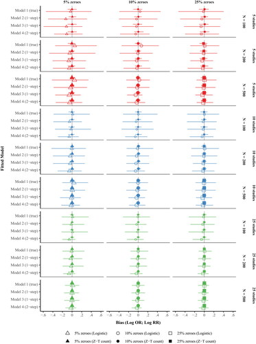
Figure 2. Coverage of the treatment effect estimates produced by hurdle negative binomial meta-analysis models by (a) fitted model, (b) hurdle sub-model, (c) no. of studies, (d) no. of participants within study, and (e) proportion of zeroes.

Notes. Model 1, the data generating model, a one-step multilevel model with study-specific intercepts and treatment slopes. Model 2, the model detailed in Huh et al., (2019), is a one-step multilevel model with a random intercept for unique study-by-treatment arm combination, where the treatment effects are calculated as post hoc contrasts of the random intercept. Model 3 is an extension of Model 2 that adds a fixed effect of treatment. Model 4 is a two-step IPD meta-analysis in which the treatment effect is estimated separately by study (step 1), and the study-specific treatment estimates and corresponding variability are subsequently modeled in a bivariate meta-analysis (step 2). Z-T count = Zero-truncated negative binomial sub-model, Logistic = Logistic sub-model.

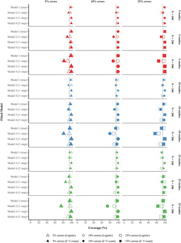
Figure 3. A sensitivity comparison of simulation results under larger treatment effect sizes (Odds Ratio [OR] = 2.01 and Rate Ratio [RR] = 0.50) compared with the original effect sizes (OR = 1.15 and RR = 0.99).

Notes. The two sets of treatment effect sizes were compared under a sample size of 10 studies, 200 participants per study, and two observations per participant at zero outcome rates of 5%, 10%, and 25%. Negative bias in the logistic sub-model and positive bias in the zero-truncated count sub-model correspond with underestimation of the true treatment effect size. Z-T count = Zero-truncated negative binomial sub-model, Logistic = Logistic sub-model.

Figure 1 summarizes the raw bias of the treatment effect estimates across the four models by (a) logistic vs. zero-truncated count sub-model, (b) number of studies, (c) sample size within study, and (d) proportion of zeroes in the outcome. The mean bias of the zero-truncated count estimates of treatment effect (see solid symbols) were within rounding error of zero for Models 1–4 across all data conditions. In contrast, there was a more pronounced bias in the logistic estimates of treatment effect (i.e., predicting no drinking vs. any drinking; see hollow symbols). The bias in the logistic portion was most pronounced in the smallest sample conditions (i.e., 5 studies and 100 participants per study), particularly with few zeroes (i.e., 5%). Additionally, there was more variability in the estimates of treatment effect in the logistic portion across all models and conditions, which was reflected by the much wider CIs. The logistic treatment effect estimates produced from the true model (Model 1) were generally within rounding error, as reflected by raw biases close to zero. However, Models 2–4 tended to underestimate the magnitude of the true treatment effect of OR = 1.15 in the logistic portion, with the greatest underestimation occurring in the smallest sample size condition with the fewest zeroes (i.e., 5 studies, 100 participants per study, 5% zeroes), at OR = 1.01 for Model 2, OR = 1.02 for Model 3, and OR = 1.03 for Model 4. When there was a small-to-modest number of studies (k = 5 or 10) and/or participants within study (N = 100 or 200), the two-step method produced more precise treatment effects with respect to no drinking (vs. drinking) than the one-step approaches, as evidenced by narrower 95% CIs for the raw bias across data conditions. However, those estimates were biased toward smaller treatment effects than the true model (Model 1).

Figure 2 summarizes the coverage of the treatment effect estimates. The coverage of Model 3 was acceptable across all data conditions, ranging from 98% to 100% across both hurdle sub-models. The coverages of Models 1 and 4 were also acceptable across most data conditions, including the true model (Model 1; Range = [92%, 100%]) and the two-step model (Model 4; Range = [91%, 100%]). The coverage of Model 2, which contains less information than Model 1 (i.e., fewer parameters to model the treatment effects), ranged from 85% to 100% for the logistic estimates and 74% to 96% for the zero-truncated count estimates of treatment effect. There was under-coverage of the zero-truncated count estimates of treatment effect from Model 2 at moderate to large within-study sample sizes (N = 200 or 500), with lower coverage at larger within-study sample sizes. However, the logistic estimates of treatment effect from Model 2 were generally acceptable, except for some under-coverage at the largest within-study sample size of 500, across the three study-level sample sizes of 5, 10, and 25.

Notably, the coverage of the treatment effects on drinking severity in Model 2 was poorer as the number of participants within each study increased. One potential explanation is that the treatment effects in Model 2 were calculated entirely from group-specific effects that were shrunken toward the overall (population) mean, resulting in greater shrinkage at larger sample size conditions, compared with Model 1. A second explanation is that the variance of the treatment effects on no drinking was underestimated in Model 2 due to the negative correlation between the random intercept and slope terms used in the data generating model (see Table 1). In other words, in studies where the average probability of not drinking was greater, the treatment effect on the probability of not drinking was smaller, reflecting typical data. In Model 2, the study-level varying intercept and slope terms from Model 1 (i.e., the data generating model) are collapsed into a single varying-intercept parameter representing unique randomized groups, from which the treatment effects are derived. Mathematically, the intercepts $u_{0g\left(B\right)}$ and $u_{0g\left(C\right)}$ from Model 2 correspond with the sum of correlated terms in Model 1, specifically ${u_{0g\left(B\right)}\approx u}_{0s\left(B\right)}+(b_{1\left(B\right)}+u_{1s\left(B\right)}){\mathrm{TREATMENT}}_{is}$ and ${u_{0g\left(C\right)}\approx u}_{0s\left(C\right)}+(b_{1\left(C\right)}+u_{1s\left(C\right)}){\mathrm{TREATMENT}}_{is},$ respectively. Because the variance of a sum of correlated terms is equal to the sum of their variance of each plus two times their covariance, a negative covariance could result in the variance of the treatment effect produced by Model 2 being underestimated.

With respect to model run time, the median durations for Models 1 to 4 were 4.5 hours, 1.8 hours, 2.0 hours, and 0.7 hours, respectively. Model 1 with N = 500 across 25 studies took the longest to run (25–26 hours). The convergence rates for Models 1 to 4 across all simulation replications were 99.8%, 100%, 100%, and 98.2%, respectively.

Sensitivity analysis

Since the simulation results presented focused on a single treatment effect on the probability of zero drinking (OR = 1.15; logistic sub-model) and the quantity of drinking when non-zero (RR = 0.99; zero-truncated count sub-model) derived from an analysis of Project INTEGRATE (see Table 1 for all simulation parameters), we conducted an additional sensitivity analysis under larger treatment effect sizes of OR = 2.01 and RR = 0.50 (i.e., log OR = 0.70 and log RR = −0.70) with a subset of the data conditions. This sensitivity analysis focused on an IPD sample size of 10 studies, 200 participants per study, and two observations per participant at each of the zero outcome rate conditions (5%, 10%, and 25%).

Figure 3 summarizes the raw bias and coverage under the original treatment effects (Figures 3a and 3b, top) for the logistic and zero-truncated count sub-models (OR = 1.15 and RR = 0.99, respectively) and larger treatment effects (Figures 3a and 3b, bottom; OR = 2.01 and RR = 0.50, respectively). The bias (Figure 3a) and coverage (Figure 3b) of the zero-truncated count estimates were acceptable and comparable across all models under the larger treatment effects. However, the logistic estimates (hollow symbols in the bottom half of Figure 3a) of Models 2–4 were underestimated under the larger treatment effect condition, which was more pronounced in Models 3 and 4. The coverage of the treatment effect estimates produced by the one-step methods was similar when the effect sizes were increased. The coverage of Model 2 tended to be lower, and that of Model 3 tended to be higher than 95%. However, the logistic estimates of treatment effect in Model 4 (hollow symbols in the bottom row of Figure 3b) had lower coverage under the larger effect size (Range = [65%, 75%]), with a larger proportion of 95% CIs not including the true value (i.e., OR = 2.01).

Discussion

Meta-analysis is an essential tool for evaluating the effectiveness of intervention approaches across multiple studies with greater accuracy and precision than single studies. IPD meta-analysis offers potential advantages over traditional meta-analysis in the ability to produce estimates of treatment effect that more properly account for count outcomes with large numbers of zeroes, which are commonplace in social behavioral and health-related research. Zero-altered outcome variables can arise when examining the frequency of a behavior, such as alcohol consumption (e.g., number of drinks consumed), suicide-related behaviors (e.g., number of suicide attempts), and sexual activity (e.g., number of condom-protected sex acts), among others. Count outcomes observed in social behavioral and health-related research frequently contain a large stack of zeroes, beyond the frequency that would be accounted for by traditional count modeling approaches such as Poisson or NB regression.

The key challenge of IPD meta-analysis is developing an analytic strategy that accurately reflects the characteristics of each study’s design and outcome measures while maintaining a consistent analytic approach across studies that may differ with respect to participant characteristics, number of treatments tested, timing of assessments, and outcome measures. If the original studies reported outcomes from an analysis that appropriately reflected outcome distributions, these outcomes could easily be combined in a traditional meta-analysis. Many of the analytic decisions detailed in this study, such as how to accommodate zero-altered count data in a longitudinal analysis, are also relevant to investigators in the context of single-study analysis. Having explained the rationale for original study investigators, we note that many advanced more appropriate models have only recently emerged. Therefore, there is a need to validly combine data from original trials that used methods that are not ideal from the current methodological perspective. IPD meta-analysis offers flexibility, yet it can be confusing to navigate through modeling options.

The present study compared four different formulations of an IPD meta-analysis utilizing multilevel hurdle NB modeling to synthesize treatment effects under various data conditions commonly encountered in social behavioral research. The two-step approach generally produced unbiased treatment effect estimates with acceptable coverage when the true effect size was small to modest (OR or RR < 1.15). However, the two-step approach tended to underestimate the treatment effect on the probability of no drinking (i.e., the logistic sub-model) when the true treatment effect was not small (OR = 2.01).

As expected, Model 1, the one-step approach used as the data generating model, performed the best across data situations. However, the key drawbacks of Model 1 are that it can only accommodate a balanced design where all studies had the same treatment conditions and a substantially greater estimation time.

To permit an IPD meta-analysis where studies evaluated different numbers or types of treatments, we evaluated two alternative one-step approaches, Models 2 and 3, which were capable of accommodating unbalanced designs across studies. We found that Model 3 produced more accurate estimates of treatment effect and corresponding intervals than Model 2, especially for the count sub-models. Specifically, Model 3 directly represented treatment assignment as a predictor in the model, which resulted in more accurately estimated credible intervals for the treatment effects (i.e., improved coverage of the true effect).

A pattern in the findings across various hurdle model-based meta-analysis approaches was that the logistic estimates tended to be more biased than the corresponding truncated count model estimates. This performance discrepancy may exist because the logistic portion of the hurdle model contains less information due to the dichotomous nature of the outcome. The degree of bias in the logistic estimates was compounded when the between- and within-study sample sizes were small to modest (i.e., five studies and/or 200 or fewer participants per study). For the truncated count model part, all four models yielded similar results.

Models 2–4 simplify the estimation of the treatment effects, compared with Model 1, the true model. For example, Model 2 represents the treatment effect with two fewer parameters by dropping the fixed slope coefficient of treatment and simplifying the clustered design by modeling study-by-treatment arm combinations as a single random intercept term. Model 3 reintroduces the fixed effect of treatment in Model 1, but retains Model 2’s simplified manner of accounting for clustering. In Model 4, the studies are analyzed separately and sequentially, the results of which are carried forward into a bivariate meta-analysis. That two-step procedure also leads to information loss, as several parameters are not carried over to the second step of Model 4, including coefficients for the covariate effects and participant-level variance parameters. Model 4 had a sizable bias and a low coverage for the logistic sub-model in the large effect size condition, especially when zero rate was small. Previous simulation research has shown poorer performance of logistic sub-models in the context of zero-inflated Poisson models (Zhou et al., 2023) and more generally in longitudinal analysis (Kim et al., 2020), although this observation warrants further investigation.

Limitations and future directions

It is important to consider the limitations of the present study. First, this simulation focused on a specific approach for modeling count data with many zeroes: hurdle NB regression. However, there are other approaches to zero-altered outcome data, including traditional zero-inflated models, which allow for zeroes in the count portion of the model (e.g., distinguishing between alcohol abstainers and drinkers who happened not to drink on a particular occasion) and newer marginalized zero-inflated approaches that produce a single set of treatment estimates, such as the marginalized zero-inflated Poisson regression model (Martin & Hall, 2017; Mun et al., 2022). Further investigation via real data analyses and simulation will be needed to assess the bias and coverage of other approaches to modeling zero-altered count outcomes in an IPD meta-analysis. Second, the present simulation assumed complete data at the participant and study levels across all approaches, so it does not provide information on the extent that the four approaches examined may be impacted by missing assessment data.

Finally, an important methodological issue in IPD meta-analysis research is how to incorporate summary-based results from completed analyses that did not properly account for zero-inflation, when the original data are not available. The recently developed Zero-inflation Bias Correction method (ZIBC method; Zhou et al., 2021) can mathematically correct biased treatment effect estimates that were improperly analyzed with the Poisson model as if they were correctly analyzed using the zero-inflated Poisson model in the original study. The ZIBC-adjusted treatment effect estimates can then be combined with IPD-derived treatment effects from other studies in the second step of a two-step IPD meta-analysis. The ZIBC method only requires summary information from the original study; however, it is limited to situations where the error was the choice of a Poisson model that ignored excessive zeroes. More methodological work and the increasing availability of IPD would help address related methodological challenges when combining data from existing studies.

Conclusions

This simulation study is the first to evaluate the accuracy and precision of IPD meta-analysis approaches for count outcomes with excessive zeroes and over-dispersion, including one-step and two-step approaches. In general, for the zero-truncated count sub-model, all models yielded similar results under all data conditions. However, for the logistic sub-model, performance varied. The true, one-step model produced the best performance while other models underestimated treatment effects on the logistic outcome. It may be unreasonable to draw a sweeping conclusion about one- vs. two-step IPD meta-analysis for count outcomes with many zeroes. The performance of both one- and two-step approaches depended on the formulation of the treatment effects, suggesting a need to carefully consider model assumptions and specifications when using IPD.

Article information

Conflict of Interest Disclosures: No authors reported any financial or other conflicts of interest in relation to the work described.

Ethical Principles: The authors affirm having followed professional ethical guidelines in preparing this work. These guidelines include obtaining informed consent from human participants, maintaining ethical treatment and respect for the rights of human or animal participants, and ensuring the privacy of participants and their data, such as ensuring that individual participants cannot be identified in reported results or from publicly available original or archival data.

Funding: The project described was supported by the National Institute on Alcohol Abuse and Alcoholism (NIAAA) grants R01 AA019511 and K02 AA028630.

Role of the Funders/Sponsors: The content is solely the responsibility of the authors and does not necessarily represent the official views of the NIAAA or the National Institutes of Health.

Acknowledgments: The ideas and opinions expressed herein are those of the authors alone, and endorsement by the authors’ institutions or the funding agencies is not intended and should not be inferred.

References

- Atkins, D. C., Baldwin, S. A., Zheng, C., Gallop, R. J., & Neighbors, C. (2013). A tutorial on count regression and zero-altered count models for longitudinal substance use data. Psychology of Addictive Behaviors, 27(1), 166–177. https://doi.org/10.1037/a0029508
- Atkins, D. C., & Gallop, R. J. (2007). Rethinking how family researchers model infrequent outcomes: A tutorial on count regression and zero-inflated models. Journal of Family Psychology, 21(4), 726–735. https://doi.org/10.1037/0893-3200.21.4.726
- Bradley, J. V. (1978). Robustness? British Journal of Mathematical and Statistical Psychology, 31(2), 144–152. https://doi.org/10.1111/j.2044-8317.1978.tb00581.x
- Burke, D. L., Ensor, J., & Riley, R. D. (2017). Meta-analysis using individual participant data: One-stage and two-stage approaches, and why they may differ. Statistics in Medicine, 36(5), 855–875. https://doi.org/10.1002/sim.7141
- Burton, A., Altman, D. G., Royston, P., & Holder, R. L. (2006). The design of simulation studies in medical statistics. Statistics in Medicine, 25(24), 4279–4292. https://doi.org/10.1002/sim.2673
- Chen, D., Liu, D., Min, X., & Zhang, H. (2020). Relative efficiency of using summary versus individual data in random‐effects meta‐analysis. Biometrics, 76(4), 1319–1329. https://doi.org/10.1111/biom.13238
- Cheng, L.-L., Ju, K., Cai, R.-L., & Xu, C. (2019). The use of one-stage meta-analytic method based on individual participant data for binary adverse events under the rule of three: A simulation study. PeerJ, 7, e6295. https://doi.org/10.7717/peerj.6295
- Debray, T. P. A., Koffijberg, H., Vergouwe, Y., Moons, K. G. M., & Steyerberg, E. W. (2012). Aggregating published prediction models with individual participant data: A comparison of different approaches. Statistics in Medicine, 31(23), 2697–2712. https://doi.org/10.1002/sim.5412
- Debray, T. P. A., Moons, K. G. M., Valkenhoef, G., Efthimiou, O., Hummel, N., Groenwold, R. H. H., & Reitsma, J. B. (2015). Get real in individual participant data (IPD) meta‐analysis: A review of the methodology. Research Synthesis Methods, 6(4), 293–309. https://doi.org/10.1002/jrsm.1160
- Gelman, A., Lee, D., & Guo, J. (2015). Stan: A probabilistic programming language for Bayesian inference and optimization. Journal of Educational and Behavioral Statistics, 40(5), 530–543. https://doi.org/10.3102/1076998615606113
- Gelman, A., Simpson, D., & Betancourt, M. (2017). The prior can often only be understood in the context of the likelihood. Entropy, 19(10), 555. https://doi.org/10.3390/e19100555
- Huh, D., Mun, E.-Y., Larimer, M. E., White, H. R., Ray, A. E., Rhew, I. C., Kim, S.-Y., Jiao, Y., & Atkins, D. C. (2015). Brief motivational interventions for college student drinking may not be as powerful as we think: An individual participant-level data meta-analysis. Alcoholism: Clinical and Experimental Research, 39(5), 919–931. https://doi.org/10.1111/acer.12714
- Huh, D., Mun, E.-Y., Walters, S. T., Zhou, Z., & Atkins, D. C. (2019). A tutorial on individual participant data meta-analysis using Bayesian multilevel modeling to estimate alcohol intervention effects across heterogeneous studies. Addictive Behaviors, 94, 162–170. https://doi.org/10.1016/j.addbeh.2019.01.032
- Jiao, Y., Mun, E.-Y., Trikalinos, T. A., & Xie, M. (2020). A CD-based mapping method for combining multiple related parameters from heterogeneous intervention trials. Statistics and Its Interface, 13(4), 533–549. https://doi.org/10.4310/SII.2020.v13.n4.a10
- Kim, S.-Y., Huh, D., Zhou, Z., & Mun, E.-Y. (2020). A comparison of Bayesian to maximum likelihood estimation for latent growth models in the presence of a binary outcome. International Journal of Behavioral Development, 44(5), 447–457. https://doi.org/10.1177/0165025419894730
- Kontopantelis, E. (2018). A comparison of one-stage vs two-stage individual patient data meta-analysis methods: A simulation study. Research Synthesis Methods, 9(3), 417–430. https://doi.org/10.1002/jrsm.1303
- Lewandowski, D., Kurowicka, D., & Joe, H. (2009). Generating random correlation matrices based on vines and extended onion method. Journal of Multivariate Analysis, 100(9), 1989–2001. https://doi.org/10.1016/j.jmva.2009.04.008
- Lin, D. Y., & Zeng, D. (2010). On the relative efficiency of using summary statistics versus individual-level data in meta-analysis. Biometrika, 97(2), 321–332. https://doi.org/10.1093/biomet/asq006
- Martin, J., & Hall, D. B. (2017). Marginal zero-inflated regression models for count data. Journal of Applied Statistics, 44(10), 1807–1826. https://doi.org/10.1080/02664763.2016.1225018
- Mathew, T., & Nordström, K. (2010). Comparison of one-step and two-step meta-analysis models using individual patient data. Biometrical Journal, 52(2), 271–287. https://doi.org/10.1002/bimj.200900143
- Mun, E.-Y., de la Torre, J., Atkins, D. C., White, H. R., Ray, A. E., Kim, S.-Y., Jiao, Y., Clarke, N., Huo, Y., Larimer, M. E., & Huh, D. (2015). Project INTEGRATE: An integrative study of brief alcohol interventions for college students. Psychology of Addictive Behaviors, 29(1), 34–48. https://doi.org/10.1037/adb0000047
- Mun, E.-Y., Jiao, Y., & Xie, M. (2016). Integrative data analysis for research in developmental psychopathology. In D. Cicchetti (Ed.), Developmental psychopathology: Theory and method (3rd ed., Vol. 1, pp. 1042–1087). Wiley. https://doi.org/10.1002/9781119125556
- Mun, E.-Y., Zhou, Z., Huh, D., Tan, L., Li, D., Walters, S. T., Tanner-Smith, E. E., Walters, S. T., & Larimer, M. E. (2022). Brief alcohol interventions are effective through 6 months: Findings from marginalized zero-inflated Poisson and negative binomial models in a two-step IPD meta-analysis. Prevention Science. Advance Online Publication. https://doi.org/10.1007/s11121-022-01420-1
- Muthén, L. K., & Muthén, B. O. (1998-2022). Mplus user’s guide (8th ed.). Muthén & Muthén.
- Perumean-Chaney, S. E., Morgan, C., McDowall, D., & Aban, I. (2013). Zero-inflated and overdispersed: What’s one to do? Journal of Statistical Computation and Simulation, 83(9), 1671–1683. https://doi.org/10.1080/00949655.2012.668550
- R Core Team. (2022). R: A language and environment for statistical computing. R Foundation for Statistical Computing. http://www.R-project.org/
- Simmonds, M. C., Higgins, J. P. T., Stewart, L. A., Tierney, J. F., Clarke, M. J., & Thompson, S. G. (2005). Meta-analysis of individual patient data from randomized trials: A review of methods used in practice. Clinical Trials, 2(3), 209–217. https://doi.org/10.1191/1740774505cn087oa
- Simmonds, M. C., Stewart, G., & Stewart, L. (2015). A decade of individual participant data meta-analyses: A review of current practice. Contemporary Clinical Trials, 45(Pt A), 76–83. https://doi.org/10.1016/j.cct.2015.06.012
- Simmonds, M. C., Tierney, J., Bowden, J., & Higgins, J. P. (2011). Meta-analysis of time-to-event data: A comparison of two-stage methods. Research Synthesis Methods, 2(3), 139–149. https://doi.org/10.1002/jrsm.44
- Stewart, G. B., Altman, D. G., Askie, L. M., Duley, L., Simmonds, M. C., & Stewart, L. A. (2012). Statistical analysis of individual participant data meta-analyses: A comparison of methods and recommendations for practice. PLoS One, 7(10), e46042. https://doi.org/10.1371/journal.pone.0046042
- Sutton, A. J., & Higgins, J. P. T. (2008). Recent developments in meta-analysis. Statistics in Medicine, 27(5), 625–650. https://doi.org/10.1002/sim.2934
- Tierney, J. F., Fisher, D. J., Burdett, S., Stewart, L. A., & Parmar, M. K. B. (2020). Comparison of aggregate and individual participant data approaches to meta-analysis of randomised trials: An observational study. PLOS Medicine, 17(1), e1003019. https://doi.org/10.1371/journal.pmed.1003019
- Wood, M. D., Fairlie, A. M., Fernandez, A. C., Borsari, B., Capone, C., Laforge, R., & Carmona-Barros, R. (2010). Brief motivational and parent interventions for college students: A randomized factorial study. Journal of Consulting and Clinical Psychology, 78(3), 349–361. https://doi.org/10.1037/a0019166
- Zhou, Z., Xie, M., Huh, D., & Mun, E.-Y. (2021). A bias correction method in meta-analysis of randomized clinical trials with no adjustments for zero-inflated outcomes. Statistics in Medicine, 40(26), 5894–5909. https://doi.org/10.1002/sim.9161
- Zhou, Z., Li, D., Huh, D., Xie, M., & Mun, E.-Y. (2023). A simulation study of the performance of statistical models for count outcomes with excessive zeros. arXiv. https://doi.org/10.48550/arXiv.2301.12674.