An Iterative Scale Purification Procedure on l_z for the Detection of Aberrant Responses

Abstract

Many person-fit statistics have been proposed to detect aberrant response behaviors (e.g., cheating, guessing). Among them, l_z is one of the most widely used indices. The computation of l_z assumes the item and person parameters are known. In reality, they often have to be estimated from data. The better the estimation, the better l_z will perform. When aberrant behaviors occur, the person and item parameter estimations are inaccurate, which in turn degrade the performance of l_z. In this study, an iterative procedure was developed to attain more accurate person parameter estimates for improved performance of l_z. A series of simulations were conducted to evaluate the iterative procedure under two conditions of item parameters, known and unknown, and three aberrant response styles of difficulty-sharing cheating, random-sharing cheating, and random guessing. The results demonstrated the superiority of the iterative procedure over the non-iterative one in maintaining control of Type-I error rates and improving the power of detecting aberrant responses. The proposed procedure was applied to a high-stake intelligence test.

Keywords:

• Person-fit statistics
• l_z
• scale purification
• aberrant behaviors
• cheating
• guessing
• item response theory

In high-stakes tests, aberrant response behaviors on items often (if not always) occur, and several types have been identified (Meijer & Sijtsma, 2001). Typical examples include (a) cheating behavior where an examinee of low ability has a high probability of correctly answering difficult items; (b) difficulty-compromise behavior where an examinee performs unexpectedly better than his or her true ability level to compromised items and; and (c) guessing behavior where an examinee randomly guesses in multiple-choice items which consequently results in an ability estimation often lower than his or her level. Failing to identify aberrant responses may have serious consequences: the resulting person parameter estimates will not accurately describe the examinee’s true latent trait levels. As a result, decisions based on these scores, such as which an individual may be admitted to college will be unfair or misleading.

A number of person-fit statistics (PFS) have been developed in the literature (Karabatsos, 2003; Meijer & Sijtsma, 2001; Rupp, 2013; Sinharay, 2017; Walker et al., 2016) to identify aberrant responses. These statistics measure the degree of agreement between an examinee’s observed response pattern and their expected response pattern based on item response theory (IRT) models. In addition to the development of PFS, robust estimators have also been introduced to counteract the adverse effects of aberrant responses. Examples of robust ability estimators include the biweight estimator (Mislevy & Bock, 1982) and the Huber estimator (Schuster & Yuan, 2011), while robust item estimators include the robust maximum marginal likelihood (RMML) estimator developed by Hong and Cheng (2019). Recently, researchers have shown great interest in incorporating robust estimators with PFS, as this approach provides a powerful method for detecting aberrant responses. For instance, Sinharay (2016) examined the use of biweight and Huber estimators in conjunction with the $l_{\mathrm{z}}^{*}$ index (Snijders, 2001), which is one of the most commonly used PFS, to identify difficulty-sharing cheating or unmotivated guessing responses. Hong and Cheng (2019) developed the RMML item estimator to identify careless responses.

This study aims to propose an iterative scale purification procedure on PFS to detect aberrant responses. It was motivated by the fact that the accuracy of PFS computation relies on accurate item and person estimates. If these estimates are distorted due to aberrant responses, the performance of PFS in detecting such responses can significantly decline. The method is inspired by similar procedures in differential item functioning (DIF) studies, which aim to obtain more accurate ability estimates for improved performance of standard DIF methods (Wang, 2008; W.-C. Wang et al., 2012). Such purification procedures have been found to substantially improve DIF assessment (French & Maller, 2007; Hidalgo-Montesinos & Gómez-Benito, 2003; Lautenschlager et al., 1994). While the purification procedure is well-established in DIF studies, its application for detecting aberrant responses is novel. To the best of our knowledge, only one study (Patton et al., 2019) employed an iterative procedure to obtain more accurate item parameter estimates to improve the detection of careless responses. Although the present work and that of Patton et al. (2019) are similar in the sense that both methods develop an iterative procedure, they differ in several significant ways. Patton et al. (2019) focused on obtaining more accurate item parameter estimates for one particular aberrant response style (i.e., carelessness), while this work aimed to obtain more accurate person estimates for three common aberrant response styles (i.e., difficulty-sharing cheating, random-sharing cheating, and random guessing). More importantly, in Patton et al. (2019), an examinee’s responses were deemed aberrant as a whole and screened from the calibration if the $l_{\mathrm{z}}^{*}$ value for the person exceeded a critical value of a significance level (e.g., −1.645). In contrast, in this study, an examinee’s responses were examined item by item, and only the responses that exceed the critical value were screened.

The current study utilizes an ability estimate derived from a purification procedure that involves iteratively removing extreme values. This estimation method can be considered a trimmed-mean estimator, which is also a type of robust estimator. Thus, the approach taken in this study shares similarities with previous PFS studies that used robust estimators (e.g., Sinharay, 2016). Note that the ability estimate is used in conjunction with the likelihood-based person-fit l_z statistic (Drasgow et al., 1985) in this study because the l_z has some appealing features (Li & Olejnik, 1997). Nevertheless, the proposed method is not confined to the specific statistic but can be conveniently generalized to other PFS.

The organization of this paper is as follows: First, the definition of the l_z is introduced. Second, the statistical distribution of the l_z and how it can be affected by the aberrant responses that lead to significantly declined performances, are elaborated. Third, the iterative purification procedure is introduced. Fourth, the performance of the proposed method is evaluated through a series of simulations, and the results are summarized. Fifth, the proposed method was applied to an empirical example. Finally, conclusions are drawn and future research direction are suggested.

A standardized likelihood-based index l_z

The l_z index is developed based on the l_o index, which represents the fit of a particular response pattern given an ability level. It is defined as (Levine & Rubin, 1979): (1) $$l_{\mathrm{o}}=\hspace{0.17em}\mathrm{\text{log}}\hspace{0.17em}\prod _{i=1}^L{P}_i{({\theta }_j)}^{u_{\mathit{\text{ij}}}}{(1-P_i({\theta }_j))}^{(1-u_{\mathit{\text{ij}}})}$$(1) where ${\theta }_j$ is the ability of examinee j; u_ij is the response to item i (i = 1, …, L) for examinee j; if the response is correct, u_ij = 1, otherwise, u_ij = 0. $P_i({\theta }_j)=P(u_{\mathit{\text{ij}}}=1|{\theta }_j)$ is the probability of scoring 1 on item i for examinee j, and it is assumed to follow a particular IRT model, for example, the three-parameter logistic model (3PL; Birnbaum, 1968): (2) $$P_i({\theta }_j)=P_i(u_{\mathit{\text{ij}}}=1|{\theta }_j)=c_i+(1-c_i)\frac{\hspace{0.17em}\mathrm{\text{exp}}\hspace{0.17em}({\alpha }_i({\theta }_j-{\delta }_i))}{1+\hspace{0.17em}\mathrm{\text{exp}}\hspace{0.17em}({\alpha }_i({\theta }_j-{\delta }_i))},$$(2) where α_i, δ_i, c_i are the discrimination, difficulty, and lower asymptote parameters of item i, respectively. To simplify the notation, let ${\mathbf{\Theta }}_i=\{{\alpha }_i,{\delta }_i,c_i\}$ be the set of item parameters. l_o, being the log-likelihood of the response pattern for an examinee, is large when the response pattern follows the model’s expectation and is small otherwise. Thus, it can be used to detect aberrant responses. It has been found that the more aberrant responses for an examinee, the better l_o will perform in detecting aberrant responses (Levine & Rubin, 1979).

As shown in Equation (1)(1) $$l_{\mathrm{o}}=\hspace{0.17em}\mathrm{\text{log}}\hspace{0.17em}\prod _{i=1}^L{P}_i{({\theta }_j)}^{u_{\mathit{\text{ij}}}}{(1-P_i({\theta }_j))}^{(1-u_{\mathit{\text{ij}}})}$$(1) , the performance of l_o is not only affected by the percentage of aberrant responses but also by θ levels, as the computation of l_o relies on θ. Therefore, the conditional distribution of l_o changes as a function of θ, and interpreting the magnitude of l_o without considering θ levels is not appropriate. For example, Drasgow et al. (1985) computed l_o using the 3PL model and the maximum likelihood (ML) estimate of ability for the responses of approximate 75,000 examinees. They found that the mean of l_o increased as θ levels increased, and the variances of l_o varied across different θ levels. To reduce the impact of θ levels on l_o, Drasgow et al. (1985) developed a standardized likelihood-based index l_z as: (3) $$l_{\mathrm{z}}=\frac{l_{\mathrm{o}}-E(l_{\mathrm{o}})}{\sqrt{\mathit{\text{Var}}(l_{\mathrm{o}})}},$$(3) where (4) $$E(l_{\mathrm{o}})=\sum _{i=1}^L(P_i({\theta }_j)\times \hspace{0.17em}\mathrm{\text{log}}\hspace{0.17em}(P_i({\theta }_j))+((1-P_i({\theta }_j))\times \hspace{0.17em}\mathrm{\text{log}}\hspace{0.17em}(1-P_i({\theta }_j)))),$$(4) (5) $$\mathit{\text{Var}}(l_{\mathrm{o}})=\sum _{i=1}^L{P}_i({\theta }_j)\times (1-P_i({\theta }_j))\times {(\hspace{0.17em}\mathrm{\text{log}}\hspace{0.17em}\frac{P_i({\theta }_j)}{1-P_i({\theta }_j)})}^2.$$(5)

The l_z index becomes popular because it is a likelihood-based function and is relatively easy to compute. More importantly, l_z is a standardized statistic and has an approximately normal sampling distribution, making hypothesis testing to determine whether a response pattern is aberrant feasible. When the normal level is set at 0.05 one-tailed, an l_z value smaller than −1.645 indicates the rejection of the null hypothesis, and the response pattern is deemed aberrant. Previous studies have demonstrated that l_z performs satisfactorily when no aberrant response is involved (good control of Type-I error rates) and when there are aberrant responses (high detection power) (Hendrawan et al., 2005; Karabatsos, 2003; Lee et al., 2014; Li & Olejnik, 1997; Reise & Due, 1991; Seo & Weiss, 2013; St-Onge et al., 2011). The power of l_z increases as the percentage of aberrant item responses increases up but decreases afterward when the percentage becomes higher. Furthermore, l_z and other PFS are more sensitive to cheating behavior (low ability examinees answer difficult items correctly) than unlucky-guessing behavior.

The statistical distribution of l_z

According to studies that have focused on the distribution of l_z (e.g., de la Torre & Deng, 2008; Noonan et al., 1992; van Krimpen-Stoop & Meijer, 1999), in theory, when all the item and person parameters are known and the test length is infinite, l_z should follow a standard normal distribution. However, in reality, the item and person parameters are seldom known and the test length is finite. As such, l_z cannot follow exactly the standard normal distribution, making it problematic to use l_z to detect aberrant responses. Even when the item and person parameters are known and the test length is long (e.g., more than 50 items), the distribution of l_z is still not symmetric but negatively skewed with positive kurtosis (Meijer & Sijtsma, 2001; Molenaar & Hoijtink, 1990; Nering, 1995; van Krimpen-Stoop & Meijer, 1999). Using l_z to detect aberrant responses becomes even more misleading when the item or person parameters are not known or not accurately estimated, especially when tests are not very long (van Krimpen-Stoop & Meijer, 1999).

As shown in Equations (1)–(5), the computation of l_z relies on the true value of θ and ${\mathbf{\Theta }}_i,$ which in reality have to be replaced with $\widehat{\theta }$ and ${\stackrel{\mathbf{⁁}}{\mathbf{\Theta }}}_i,$ respectively. Researchers (Nering, 1995; Reise, 1995; Snijders, 2001) compared the l_z distributions when the true θ and the estimated $\widehat{\theta }$ are used, assuming all item parameters are known. When θ is used, the mean and variance of the l_z distribution under the null condition (no aberrant response) are very close to the expected value of 0 and 1, respectively. In contrast, when $\widehat{\theta }$ is used, the mean is consistently larger than 0 and the variance is smaller than 1. As a results, the empirical Type-I error rates of using l_z to detect aberrant responses are lower than nominal levels.

Researchers have adopted different methods to tackle the problem that the distribution of l_z does not exactly follow the standard normal distribution when $\widehat{\theta }$ (instead of θ) is used. These methods can be generally classified into two approaches: (1) methods to obtain more accurate $\widehat{\theta },$ and (2) methods to correct the empirical distribution of l_z. Theoretically, if $\widehat{\theta }$ can be estimated more accurately, the empirical distribution will become closer to standard normal distribution.

For the first approach, researchers typically utilize various methods to mitigate or reduce the impact of aberrant responses on ability estimation. For example, some studies (Glas & Dagohoy, 2007; X. Wang et al., 2017) have incorporated a correction to $\widehat{\theta }$ to account for such effects. In this study, the same approach is adopted, but with the iterative purification of $\widehat{\theta }.$ For the second approach, researchers usually use statistical or nonstatistical methods to make the empirical distribution of l_z approximate the standard normal distribution. One representative of this approach is the $l_{\mathrm{z}}^{*}$ index (Snijders, 2001), which yields the asymptotical standardization of l_z with estimated ability parameter. The Type-I error rates of using $l_{\mathrm{z}}^{*}$ were found to be closer to nominal levels than those of using l_z and other PFS (de la Torre & Deng, 2008; Magis et al., 2012; Snijders, 2001). On the other hand, de la Torre and Deng (2008) proposed to derive the empirical distribution of l_z based on $\widehat{\theta }$ through a resampling method. It was found that the resampling-based l_z has Type-I error rates close to the nominal value for most ability levels.

The iterative scale purification procedure for l_z

In this study, we propose an iterative scale purification procedure to obtain an accurate $\widehat{\theta }$ for improved performance of l_z. As such, $\widehat{\theta }$ is closer to θ, the calculation of the l_z will be more accurate. Assume examinee j has responded to a test with L (dichotomous) items. The person will receive an ability estimate (${\widehat{\theta }}_j$) according to a particular IRT model, based on ML estimation or Bayesian methods (BM). For each item i and each examinee j, we can calculate: (6) $$Z_{\mathit{\text{ij}}}^2\equiv \frac{{(u_{\mathit{\text{ij}}}-E(u_{\mathit{\text{ij}}}))}^2}{\mathit{\text{Var}}(u_{\mathit{\text{ij}}})},$$(6) where $E({\mu }_{\mathit{\text{ij}}})=P({\widehat{\theta }}_j),$ $\mathit{\text{Var}}(u_{\mathit{\text{ij}}})=u_{\mathit{\text{ij}}}^2(1-P({\widehat{\theta }}_j))+{(1-u_{\mathit{\text{ij}}})}^{2}P({\widehat{\theta }}_j),$ and others are defined as those in Equation (1)(1) $$l_{\mathrm{o}}=\hspace{0.17em}\mathrm{\text{log}}\hspace{0.17em}\prod _{i=1}^L{P}_i{({\theta }_j)}^{u_{\mathit{\text{ij}}}}{(1-P_i({\theta }_j))}^{(1-u_{\mathit{\text{ij}}})}$$(1) . As described in Embretson and Reise (2000), $Z_{\mathit{\text{ij}}}^2$ approximately follows the χ² distribution with one degree of freedom. To identify aberrant responses, different cutoff (C) can be used for screening, depending on the criteria levels. For example, C are 1.64, 2.71, and 3.84 for criteria levels of 0.80, 0.90, and 0.95, respectively. To simplify notations, they are denoted as C₈₀, C₉₀, and C₉₅, respectively. A response with $Z_{\mathit{\text{ij}}}^2$ larger than a predefined C would be deemed aberrant.

Because the estimation of person and item parameters relies on each other, the iterative purification procedure is used. As illustrated in Figure 1, the procedure proceeds as follows:

Figure 1. An illustrative diagram of iterative scale purification procedure.

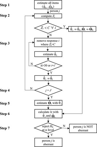
1. Obtain ability and item parameter estimates based on an examinee’s responses to all items using a certain program for IRT analysis (e.g., mirt R package [Chalmers, 2012]), denoted as ${\widehat{\theta }}_0$ and ${\stackrel{\mathbf{⁁}}{\mathbf{\Theta }}}_0,$ respectively;

2. Use Equation (6)(6) $$Z_{\mathit{\text{ij}}}^2\equiv \frac{{(u_{\mathit{\text{ij}}}-E(u_{\mathit{\text{ij}}}))}^2}{\mathit{\text{Var}}(u_{\mathit{\text{ij}}})},$$(6) to judge every item response for aberrancy using a predefined cutoff C. If no item response was identified as aberrant, the ${\widehat{\theta }}_0$ and ${\stackrel{\mathbf{⁁}}{\mathbf{\Theta }}}_0$ obtained from Step 1 will be treated as the final ${\widehat{\theta }}_j$ and ${\stackrel{\mathbf{⁁}}{\mathbf{\Theta }}}_i;$

3. Remove those item responses judged as aberrant in Step 2 from the test, and update ${\widehat{\theta }}_j$ based on the responses to the remaining items;

4. Repeat Steps 2 and 3 until the same set of item responses is judged as aberrant at two consecutive iterations or a maximum number of iterations (say, 10) is reached;

5. Estimate ${\stackrel{\mathbf{⁁}}{\mathbf{\Theta }}}_i$ with the final ${\widehat{\theta }}_j;$

6. Use ${\widehat{\theta }}_j$ and ${\stackrel{\mathbf{⁁}}{\mathbf{\Theta }}}_i$ to calculate l_z across all items;

7. Compare the l_z to the critical value (e.g., –1.645 at the .05 nominal level, one-tailed) to determine whether the response pattern is aberrant. Alternatively, the distribution of l_z can be obtained through a resampling method: simulate a large number of response patterns (e.g., 1,000) based on the final ${\widehat{\theta }}_j$ and ${\stackrel{\mathbf{⁁}}{\mathbf{\Theta }}}_i$ according to an IRT model of interest, and compute the l_z value for each simulated response pattern. If the empirical l_z is smaller than the 95th percentile of the simulated l_z values (when the nominal level is set at .05, one-tailed), the response pattern is deemed aberrant.

To implement the iterative scale purification procedure, we developed a computer program in the R environment, which embeds different IRT models (Rasch, 1960, 2PL, 3PL), ability methods (“ML”, “BM”), cutoff values, number of iterations, normal distribution or resampling distribution, and so on. The program is available upon request from the first author.

Simulations

A series of simulations were conducted to evaluate the iterative procedure. Two conditions were intentionally designed: item parameters known and item parameters unknown. In the first condition, the true (generating) item parameters are used assuming they are known. This condition mimics previous studies (e.g., Nering, 1995; Reise, 1995; Snijders, 2001) and represents the ideal condition where items parameters do not contain measurement errors. The purpose of this condition was to evaluate the performances of the iterative procedure in improving the accuracy of different levels of $\widehat{\theta }.$ In the second condition, item parameters are treated as unknown. This condition represents the condition in reality where item and person parameters are simultaneously estimated and inevitably contain some measurement errors. The purpose was to evaluate the performances of the iterative procedure in the detection of aberrant patterns, compared to the traditional l_z. The critical values of l_z were derived using the resampling method in both conditions where 1,000 samples were simulated and the nominal level is set at 0.05 (one-tailed).

Condition I: Item parameters known

Four independent variables were manipulated in the study: (a) methods: traditional l_z (Equation (3)(3) $$l_{\mathrm{z}}=\frac{l_{\mathrm{o}}-E(l_{\mathrm{o}})}{\sqrt{\mathit{\text{Var}}(l_{\mathrm{o}})}},$$(3) ) and l_z with the iterative purification procedure using cutoff C₈₀, C₉₀, and C₉₅; (b) proportions of items with aberrant responses (PIAR): 0, 0.1, 0.2, 0.3, and 0.4, where PIAR = 0 suggested no aberrant response and serves as the null condition and PIAR = 0.1 indicated the examinee had aberrant responses to 10% of the items, and so on; (c) IRT model: Rasch model and 3PL model; (d) aberrance style: difficulty-sharing cheating, random-sharing cheating, and random guessing. A total of 40 dichotomous items were generated. In the difficulty-sharing cheating scenario, only the most difficult items were compromised. For example, when PIAR = 0.1, the four most difficult items were compromised (i.e., a correct answer was guaranteed). In the random-sharing cheating scenario, the top 50% of the hardest items in the test had the same probability of being compromised, and the compromised items were randomly selected. A correct answer was guaranteed to the selected items. In the random guessing scenario, the top 50% of the hardest items in the test had the same probability of being guessed, and the randomly selected items to be guessed had a success probability of .20. For each of the selected items, the response was randomly generated from the Bernoulli distribution with p = 0.20.

The θ values were set as −3, −2, −1, 0, 1, 2, and 3, each with 1,000 replications (examinees). The item difficulty parameters were randomly drawn from the standard normal distribution. The EAP estimates were computed for person measures, with a prior distribution N (0, 1). The item parameters were treated as known in obtaining the EAP estimates. Therefore, Step 5 in the iterative scale purification procedure is skipped in this condition. The nominal level 0.05 was used for l_z in Step 7 in the iterative procedure.

For the null condition, the outcome variable was the Type-I error rate which was computed as the percentage of examinees among the 1,000 examinees that were mistakenly detected as having aberrant responses. Otherwise, the outcome variable was the detection accuracy (power) rate, defined as the percentage of examinees that were correctly detected as having aberrant responses. Only when the Type-I error rate was well-controlled (e.g., at the 0.05 nominal level) would the power rate be meaningful.

Condition II: Item parameters unknown

Under this condition, a total of 1,000 examinees were generated from N (0, 1). In addition to the four independent variables in Condition I, the percentages of examinees with aberrant responses (PEAR) was also manipulated. The PEAR levels for 3PL model (see Table 3) were set lower than those for Rasch model (see Table 2) because it was found in our pilot studies that the estimation for 3PL model was very poor when there was high PEAR. For example, the discrimination parameter estimates became negative when PEAR levels were higher than 0.3 for difficulty-sharing cheating and random-sharing cheating scenarios.

Table 2. Type-I error rates (in %) in the difficulty-sharing (DS), random-sharing (RS) and random guessing (RG) scenarios with Rasch model in Condition II.

		PEAR	0	0.1				0.2				0.3				0.4				0.5
	Iteration	PIAR	0	0.1	0.2	0.3	0.4	0.1	0.2	0.3	0.4	0.1	0.2	0.3	0.4	0.1	0.2	0.3	0.4	0.1	0.2	0.3	0.4
DS	lz		4.8	1.9	0.4	0.2	0.3	1.4	0.3	0.0	0.1	2.1	0.6	0.0	0.0	2.5	1.0	0.5	0.0	4.4	2.6	2.4	0.2
	C95		5.6	2.6	1.0	0.7	0.6	2.3	0.8	0.4	0.1	2.6	0.7	0.0	0.0	2.5	1.2	0.8	0.0	5.6	3.8	2.2	0.0
	C90		5.3	2.8	1.3	1.3	1.0	3.3	1.5	0.6	0.1	2.7	1.1	0.0	0.1	2.5	1.3	0.8	0.0	6.2	4.0	2.4	0.0
	C80		5.8	4.2	2.4	2.3	1.7	4.4	2.4	1.8	0.9	4.9	2.0	0.6	0.4	3.8	2.3	2.3	1.2	8.4	7.2	5.2	1.4
RS	lz		4.8	3.1	2.3	1.9	1.9	1.8	1.9	0.8	0.8	2.1	0.1	0.6	0.3	1.2	0.7	0.2	0.0	0.2	0.2	0.2	0.0
	C95		5.6	4.4	3.6	2.9	3.0	2.8	2.3	2.0	1.4	2.9	0.4	0.7	0.6	1.8	1.0	0.3	0.2	0.6	0.4	0.2	0.0
	C90		5.3	4.7	4.0	3.3	3.2	3.6	2.8	2.0	1.5	3.7	0.6	0.9	0.7	1.8	1.2	0.5	0.5	0.6	0.4	0.2	0.0
	C80		5.8	5.9	5.1	4.8	4.1	4.5	3.9	2.9	2.4	4.9	1.4	1.3	1.4	2.7	1.3	1.0	0.7	1.4	0.8	0.4	0.2
RG	lz		4.8	4.7	4.1	3.2	3.2	2.6	2.5	1.5	1.5	4.0	2.9	1.0	0.4	2.5	1.3	0.8	0.7	0.8	0.6	0.6	0.2
	C95		5.6	6.7	5.6	4.2	3.7	3.9	3.3	2.3	2.6	5.1	4.0	1.6	0.6	3.5	1.7	1.3	0.7	1.4	1.4	1.8	0.4
	C90		5.3	7.0	5.9	4.8	4.6	4.3	3.6	3.0	3.1	5.3	4.0	2.3	1.0	3.7	2.3	1.5	0.7	2.0	1.6	1.8	0.4
	C80		5.8	8.1	7.1	5.2	6.2	5.9	4.4	4.4	3.8	6.7	5.3	4.0	1.3	4.2	3.2	2.0	0.7	2.8	2.0	2.0	0.6

Note. PIAR: Percentage of items with aberrant responses; PEAR: Percentage of examinees with aberrant responses.

Table 3. Type-I error rates (in %) under the difficulty-sharing (DS), random-sharing (RS) and random guessing (RG) scenarios with 3PL model in Condition II.

		PEAR	0	0.05					0.1					0.15					0.2
	Iteration	PIAR	0	0.1	0.15	0.2	0.25	0.3	0.1	0.15	0.2	0.25	0.3	0.1	0.15	0.2	0.25	0.3	0.1	0.15	0.2	0.25	0.3
DS	lz		4.8	3.7	3.2	2.7	3.7	2.2	4.1	4.9	4.8	4.6	2.5	4.3	4.9	5.8	6.9	6.2	4.7	5.2	5.8	7.4	8.4
	C95		6.3	5.6	4.8	2.7	3.8	2.2	5.7	5.5	2.8	3.6	2.2	5.7	5.8	5.5	5.5	8.0	6.7	13.4	11.4	14.7	19.4
	C90		6.4	5.2	4.9	2.1	5.2	2.3	6.0	6.0	4.9	2.8	1.8	6.4	6.8	6.1	5.4	8.6	6.6	13.8	10.1	16.8	20.3
	C80		6.6	5.8	5.1	2.4	5.4	3.1	5.5	5.3	3.7	2.7	2.7	5.9	7.7	8.4	8.6	9.3	8.5	16.4	12.3	30.2	35.1
RS	lz		4.8	4.2	3.7	3.4	3.2	2.8	4.5	4.1	4.1	3.5	3.3	4.7	5.1	5.5	5.0	4.5	4.0	4.3	3.8	4.6	5.9
	C95		6.3	5.9	5.5	5.1	4.3	4.2	6.6	5.3	4.8	3.9	3.4	7.6	8.7	8.8	8.7	8.9	8.8	10.6	9.3	9.6	13.5
	C90		6.4	5.9	5.4	5.0	4.5	4.1	6.9	5.6	5.4	4.4	4.4	8.4	9.1	8.9	9.1	9.4	9.7	10.8	9.9	10.9	19.9
	C80		6.6	8.8	5.7	6.1	5.8	4.9	6.9	6.0	5.5	5.0	4.5	8.5	9.7	9.7	9.5	9.7	10.5	12.1	10.4	12.1	20.6
RG	lz		4.8	4.3	4.5	4.1	3.7	3.7	3.9	3.6	3.1	3.2	3.0	4.1	3.8	3.5	3.3	2.9	3.5	3.7	2.7	2.6	2.2
	C95		6.3	6.4	6.5	6.0	6.2	5.9	5.7	5.4	5.2	5.8	4.5	6.4	5.9	5.7	4.8	4.7	5.8	5.7	4.9	5.1	4.6
	C90		6.4	7.5	7.4	7.2	6.8	6.5	6.7	6.9	6.1	5.9	6.3	6.9	6.4	6.5	6.3	5.8	6.5	6.5	6.5	5.6	5.7
	C80		6.6	9.1	8.5	8.5	7.9	8.2	8.8	8.1	8.2	8.5	8.1	8.7	8.8	8.1	7.6	7.3	9.4	9.0	8.1	7.5	7.7

Note. PIAR: Percentage of items with aberrant responses; PEAR: Percentage of examinees with aberrant responses.

All item and person parameters were simultaneously estimated using standard EM algorithm and person parameters were estimated using EAP estimation. In the non-iterative procedure, item and person measures were used directly to compute l_z; whereas in the iterative procedure, both item and the person measures were updated iteratively (as shown in Figure 1) using the customized program. A total of 100 replications were run under each condition, and all 1,000 examinees were subject to aberrancy inspection. The major outcome variable was the Type-I error rate and power rate.

Additionally, it was interesting to know whether θ could be more accurately estimated with the iterative procedure than the non-iterative procedure. The mean error (ME) and mean square error (MSE) for $\widehat{\theta }$ were computed to demonstrate the advantage of the iterative procedure over the non-iterative one. When there were aberrant responses, the ME and MSE for the examinees without aberrant responses (normal examinees) and those with aberrant responses (aberrant examinees) were computed separately.

Expected results of the simulations

We had the following major expectations. First, under the null condition, the Type-I error rate would be near the expected nominal level. Second, the detection accuracy (power) would be improved by the iterative procedure given that the more accurate $\widehat{\theta }$ was obtained. Third, the smaller the cutoff C for $Z_{\mathit{\text{ij}}}^2,$ the larger the PIAR, and the smaller the PEAR (Condition II), the higher the detection accuracy would be. Aberrant responses would be easier to be screened by a smaller C because the smaller the C, the smaller the Type-II error rate and the higher the power. A larger PIAR indicated the examinee had a higher percentage of aberrant responses to items and, thus, was easier to be detected. When PEAR was small, the item parameters would be accurately estimated, which in turn would help the detection.

Fourth, in the difficulty-sharing and random-sharing cheating scenarios, the lower the θ level, the higher the power. An examinee with a low θ level but answered difficult items correctly was considered more aberrant than an examinee with a high θ level, making the detection of lower θ levels easier. In the random-guessing scenario, the higher the θ level, the easier the detection. An examinee with a high θ level but answered items correctly at a chance level (random guessing) was considered more aberrant than an examinee with a low θ level.

Fifth, the power in the difficulty-sharing cheating scenario would be the highest among the three scenarios, followed by that in the random-sharing cheating scenario, and the power in the random guessing scenario would be the lowest. In the difficulty-sharing cheating scenario, the aberrancy was mainly on answering very difficult items correctly, resulting in a large misfit. In the random-sharing cheating scenario, even easy items were compromised, and answering easy items correctly would not result in a large misfit. In the random guessing scenario, the aberrancy was equally distributed across items and examinees, resulting in a small misfit.

Results

Condition I: Item parameters known

Figure 2 shows the type-I error rates in the null condition while Figures 3 and 4 show the power rates in the difficulty-sharing cheating, the random-sharing cheating, and the random-guessing for Rasch and 3PL models, respectively.

Figure 2. Type-I error rates in the null condition with Rasch (left panel) and 3PL (right panel) models in Condition I.

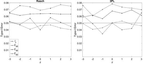
Figure 3. Power rates in the difficulty-sharing cheating (left panel), random-sharing cheating (middle panel) and random guessing (right) scenarios with Rasch model in Condition I, and with PIAR =0.1 (top panel) and PIAR =0.4 (bottom panel). Note. PIAR: Percentage of items with aberrant responses.

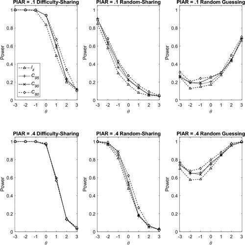
Figure 4. Power rates in the difficulty-sharing cheating (left panel), random-sharing cheating (middle panel) and random guessing (right) scenarios with 3PL model in Condition I, and with PIAR =0.1 (top panel) and PIAR =0.4 (bottom panel). Note. PIAR: Percentage of items with aberrant responses.

The null condition

The Type-I error rates in the null condition, as shown in Figure 2, were near the expected nominal level (i.e., 0.05) across θ levels for both Rasch and 3PL models. Moreover, smaller values of C (e.g., C₈₀) resulted in higher Type-I error rates because a response is more likely to be screened with a smaller cutoff value. These results met our expectations.

The difficulty-sharing cheating scenario

The iterative procedure resulted in a significant improvement in power rates compared to the non-iteration procedure using the standard l_z index. Take 3PL model as an example. When PIAR = 0.1 (top and left panel, Figure 4), the power rate for θ = 0 was 0.914, 0.693, and 0.483, respectively, for C₈₀, C₉₀, and C₉₅. Compared to the traditional l_z index (non-iteration procedure) where the power rate was 0.305, the power improvement ratio was 1.997, 1.271, and 0.585, respectively, for C₈₀, C₉₀, and C₉₅. However, the improvement was less noticeable when PIAR = 0.4 (bottom and left panel, Figure 4) or when θ < −1. This was because when PIAR = 0.4 the amount of aberrancy was too high for Z_ij to perform appropriately; when θ < −1, even the standard l_z index would yield a perfect power, leaving no room for improvement with the iteration procedure.

The lines in the left panel of Figures 3 and 4 show a general decreasing trend, indicating that the power rates are higher for lower θ level for both iterative and non-iterative procedures in the difficulty-sharing cheating scenario. For instance, for the condition of PIAR = 0.1 under 3PL model, the power rates for θ = −3, −2, −1, 0, 1, 2, and 3 were 0.982, 0.998, 0.861, 0.915, 0.919, 0.833 and 0.173, respectively, for C₈₀; they were 0.873, 0.678, 0.546, 0.305, 0.205, 0.208, and 0.009, respectively, for l_z. The power rates of the iterative procedure were uniformly higher than those of the non-iterative procedure. Moreover, in Figures 3 and 4, the power rates for PIAR = 0.4 were higher than those for PIAR = 0.1, indicating that a larger PIAR resulted in a higher power rate.

A comparison of Figures 3 and 4 revealed that in the difficulty-sharing cheating scenario, the general patterns for Rasch model (left panel, Figure 3) are similar to those for 3PL model (left panel, Figure 4). However, the improvement yielded by the iteration procedure under Rasch model seems to be smaller than that under 3PL model. Moreover, Rasch model has higher power rates than 3PL model because the $\widehat{\theta }$ are more accurately estimated for Rasch model.

The random-sharing cheating scenario

According to Figures 3 and 4, the major findings on the power rates in the random-sharing cheating scenario were very similar to those in the difficulty-sharing cheating scenario. There were, however, two major differences. First, the improvement made by the iteration procedure was more significant in the random-sharing cheating scenario, especially for 3PL model. For example, when PIAR = 0.1 under 3PL model (top and middle panel, Figure 4), the power rates for θ = 0 were 0.473, 0.281, and 0.168, respectively, for C₈₀, C₉₀, and C₉₅. The power improvement ratio compared to the standard l_z index (0.084) was 4.631, 2.345, and 1.000, respectively, which were substantially larger than those found in the difficulty-sharing cheating scenario. Second, the power rates were smaller in the random-sharing cheating scenario. For example, for PIAR = 0.1 under 3PL model, the average power rate for θ = 0 across different methods was about 0.277 (the mean of 0.473 [C₈₀], 0.281 [C₉₀], 0.168 [C₉₅], and 0.084 [l_z]) in the random-sharing cheating scenario. It was smaller than that in the difficulty-sharing cheating scenario, which was 0.599 (the mean of 0.914 [C₈₀], 0.693 [C₉₀], 0.483 [C₉₅], and 0.305 [l_z]).

The random guessing scenario

The right panels in Figures 3 and 4 reveal that the patterns of power rates across θ levels in the random guessing scenario were opposite to those in the difficulty-sharing and the random-sharing cheating scenarios. The increasing lines suggest that, in general, the higher the θ level, the higher the power. This is because random guessing behavior is not aberrant in the same sense as the difficulty-sharing or random-sharing cheating behaviors. Guessing behavior is more likely to be used as an answering strategy by low-ability students who find the items too difficult. Therefore, it caused more dramatic misfit for examinees with high ability levels than for those with low ability levels.

Moreover, the iteration procedure showed significant improvements in power rates, particularly for examinees with high θ levels and for a larger PIAR. For example, for PIAR = 0.1 under 3PL model (right and top panel, Figure 4), the power rates for θ = 3 were 0.677, 0.630, 0.624, and 0.347, respectively, for C₈₀, C₉₀, C₉₅, and l_z. Thus, the power improvement ratios were 0.948, 0.814, and 0.796, respectively, for C₈₀, C₉₀, and C₉₅. When PIAR = 0.4 (right and bottom panel, Figure 4), the powers rates were 0.996, 0.991, 0.521, and 0.349, respectively, for C₈₀, C₉₀, C₉₅. Thus, the power improvement ratios increase to 1.852, 1.608, and 0.492, respectively, for C₈₀, C₉₀, and C₉₅.

A comparison of the right panels in Figures 3 and 4 shows an interesting phenomenon when using different IRT models. For Rasch model, the power rates decrease between θ = −3 and θ = −2 but increase afterward as θ gets larger. In contrast, for 3PL model, the power rates increase almost steadily as θ increases. To interpret this phenomenon, we computed the averaged success probabilities across items using the generating item parameters for different ability levels. As shown in Table 1, the success probability for θ = −2 with Rasch model is 0.221, which is very close to the probability of success in the random guessing scenario that was set to be .20. As such, although we simulate the random-guessing aberrancy for θ = −2 with Rasch model, the responses were very approximate to the responses without aberrancy because they have similar success probabilities. In other words, the misfit was small for θ = −2 under Rasch model, leading to difficulty in detection. Therefore, the lowest detection power rate was found for θ = −2 under Rasch model. Likewise, for 3PL model, the success probability for θ = −3 (0.203) is close to the fixed successful probability in the random guessing scenario. Therefore, the lowest detection power rate was found for θ = −3 under 3PL model.

Table 1. Averaged successful probability for different ability levels (θ) with Rasch and three-parameter logit (3PL) models in Condition I.

	θ = –3	θ = –2	θ = –1	θ = 0	θ = 1	θ = 2	θ = 3
Rasch	.123	.221	.340	.470	.605	.737	.851
3PL	.203	.313	.464	.621	.758	.861	.927

Condition II: Item parameters unknown

Type-I error rate

When none of the examinees exhibited aberrant responses (PIAR = 0; PEAR = 0; whole data were clean), the Type-I error rate was 4.8% for both Rasch (Table 2) and 3PL (Table 3) models, when no iteration was implemented (i.e., l_z). These empirical rates were very close to the expected value of 5%. When the iterative procedure was implemented, the Type-I error rate increased slightly. The Type-I error rates were 5.6%, 5.3%, and 5.8% under Rasch model, and 6.3%, 6.4%, and 6.6% under 3PL model, respectively, when C₉₅, C₉₀, and C₈₀ were used. Slight inflation suggests that when no examinees exhibited aberrant responses, using the iterative procedure, although unnecessary, did little harm.

When some examinees had aberrant responses, in general, the Type-I error rates remained at the 5% nominal level when the PIAR and PEAR were small for both noniterative and iterative procedures. However, when the PIAR and PEAR increased, the estimation for item parameters was adversely affected by those examinees with aberrant responses, leading to less well-controlled Type-I error rates.

Specifically, for the difficulty-sharing cheating and random-sharing cheating scenarios, for the standard l_z, the Type-I error rates under Rasch model (Table 2) become very conservative when the percentages of aberrancy increase but become inflated under 3PL model (Table 3). For the iterative procedures, under Rasch model (Table 2), the Type-I error rates were also conservative, but with a smaller magnitude than those of the standard l_z (i.e., closer to the nominal level); Under 3PL model (Table 3), except for PEAR = 2., the Type-I error rates inflated more than those of the standard l_z, but remained at an acceptable level. Overall, it appeared that the iterative procedure yielded better control of Type-I error rates than the non-iterative procedure.

Power rate

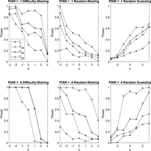
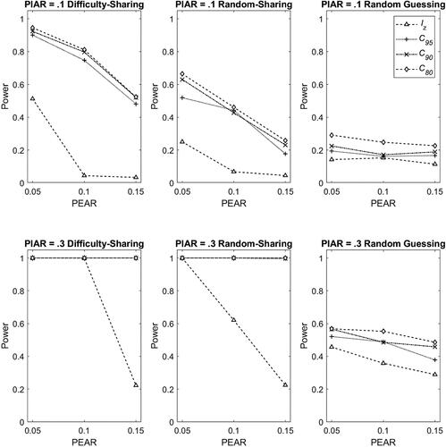
The power rates for the three scenarios are presented in Figures 5 and 6. Note that the power rates for PEAR = 0.2 under 3PL model were not shown because the power rates are meaningless when the Type-I errors in this condition were inflated. The general findings were very similar across scenarios and matched our expectations: the iterative procedure improved the power substantially; the smaller cutoff C, the larger the PIAR, and the smaller the PEAR, the higher the power would be. A comparison of the three scenarios indicated that the difficulty-sharing cheating scenario yielded the highest power, followed by the random-sharing scenario, and the random guessing scenario. This was consistent with that was found in the previous condition of known item parameters.

Figure 5. Power rates in the difficulty-sharing cheating (left panel), random-sharing cheating (middle panel) and random guessing (right panel) scenario with Rasch model in Condition II, and with PIAR =0.1 (top panel) and PIAR =0.4 (bottom panel). Note. PIAR: Percentage of items with aberrant responses; PEAR: Percentage of examinees with aberrant responses.

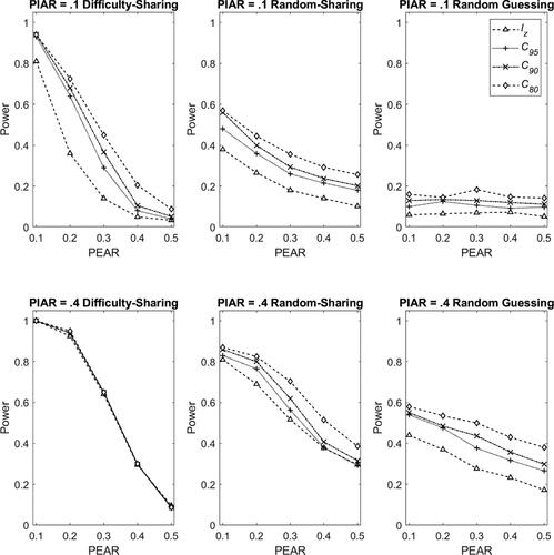
Figure 6. Power rates in the difficulty-sharing cheating (left panel), random-sharing cheating (middle panel) and random guessing (right panel) scenario with 3PL model in Condition II, and with PIAR =0.1 (top panel) and PIAR =0.3 (bottom panel). Note. PIAR: Percentage of items with aberrant responses; PEAR: Percentage of examinees with aberrant responses. The results for PEAR = .2 are not shown because the Type-I errors in this condition were inflated.

Accuracy of ability estimation

It was found that when there was no aberrant response, the ME and MSE of $\widehat{\theta }$ for both the iterative and non-iterative procedures were small and close, suggesting that both procedures yielded accurate $\widehat{\theta }.$ However, when there were aberrant responses, the iterative procedure yielded more accurate $\widehat{\theta }$ for aberrant examinees than the non-iterative procedure, especially when there was high percentage of aberrant responses.

For illustration, the ME and MSE of $\widehat{\theta }$ from the iterative procedure using C₈₀ and tradition l_z under the condition of difficulty-sharing and Rasch model are compared. When there was no aberrant response, the ME and MSE were −0.037 and 0.190, respectively, for the iterative procedure, and 0.003 and 0.139, respectively, for the traditional l_z, indicating that both the iterative and non-iterative procedures yielded accurate $\widehat{\theta }.$ When there were aberrant responses and the percentage of aberrant responses was low (e.g., PIAR = 0.1 and PEAR = 0.1), the ME and MSE for normal examinees were −0.052 and 0.167, respectively, in the iterative procedure, and −0.022 and 0.140, respectively, in the traditional l_z, suggesting the iterative procedure did little harm to the person estimation of normal examinees. In contrast, the ME and MSE for aberrant examinees were 0.799 and 1.570, respectively, in the iterative procedure, and 1.490 and 2.331, respectively, in the traditional l_z, indicating the iterative procedure was very effective in improving the person estimation of aberrant examinees.

When the percentage of aberrant responses was high (e.g., PIAR = 0.1, and PEAR = 0.3), the ME and MSE for normal examinees were −0.209 and 0.719, respectively, in the iterative procedure, and −0.293 and 0.747, respectively, in the traditional l_z, suggesting the iterative procedure did little harm. In contrast, the statistics for aberrant examinees were 2.340 and 5.593, respectively, in the iterative procedure, and 2.600 and 10.497, respectively, in the traditional l_z, suggesting an improvement in the person estimation of aberrant examinees with the iterative procedure. In short, although not perfect, the iterative procedure was effective in person estimation and the detection of aberrant responses.

An empirical example

The data was retrieved from the R package ‘PerFit’ (Tendeiro, 2021), which consists of dichotomous responses of 1,000 examinees to a high-stake 26-item intelligence test on number completion in Dutch. The item and person parameters were simultaneously estimated with the 3PL model. Four procedures were implemented to examine person fit for each person: traditional l_z and l_z with the iterative purification procedure using cutoff C₈₀, C₉₀, and C₉₅. Two nominal levels, as in, 0.05 and 0.01, were used with l_z in the procedures.

The results showed that the item discrimination estimates are in the range of 0.598 and 1.859 (M = 1.111, SD = 0.345), the item difficulty estimates are between −2.120 and 3.130 (M = 0.242, SD = 1.380), and the guessing parameter estimates are between 0.000 and 0.779 (M = 0.109, SD = 0.212). Due to space constraints, the detailed results are provided in Table A1 in the online supplement. The aberrancy rate for the four procedures were 0.055 (l_z), 0.081 (C₈₀), 0.076 (C₉₀), and 0.061 (C₉₅), respectively, when the nominal level 0.05 was used, and were 0.020 (l_z), 0.030 (C₈₀), 0.026 (C₉₀), and 0.021 (C₉₅), respectively, when the nominal level 0.01 was used. To evaluate the agreement of aberrancy detection between the procedures, Cohen’s Kappa coefficients were calculated and are shown in Table 4, where the results from the nominal level 0.05 are in the upper triangle and those from the nominal level 0.01 in the lower triangle.

Table 4. Agreement between four procedures for aberrancy detection in empirical example.

	lz	C95	C90	C80
lz	–	0.945	0.829	0.795
C95	0.975	–	0.883	0.849
C90	0.867	0.891	–	0.965
C80	0.795	0.819	0.927	–

Note. The results with nominal level 0.05 are in the upper triangle and those with nominal level 0.01 are in the lower triangle.

Particular results worth noting are: First, results from both nominal levels indicate that the traditional lz has the largest agreement coefficient with iterative lz using C₉₅ and the smallest agreement coefficient with iterative lz using C₈₀ in detecting aberrant examinees, which meet our expectations. Second, the coefficients suggest the substantial or almost perfect agreements between the four procedures for aberrancy detection in this example, especially when the nominal level 0.05 was used.

To demonstrate the consistency and inconsistency of aberrancy detection results when using the four procedures, six examinees were selected and their sorted responses with descending item difficulties, ability estimates from the traditional lz and iterative lz using C₈₀, and detection results when the nominal level 0.05 was used are shown in Table 5. Examinee #278 answered many difficult items correctly but failed many less difficult items, whereas examinee #772 seemed to answer the items correctly in a random pattern. These two examinees were detected as aberrant by all of the four procedures. Likewise, examinees #709, #69, and #237 seemed to have some unusual responses, but none of them were detected by the traditional lz. Furthermore, examinee #742 was detected as aberrant only by the iterative procedure with a smaller C. Note that a smaller C is more likely to lead to higher Type-I error rates, as the simulation study reveals. More evidence (e.g., classroom performances) should be taken into account when judging whether the examinees are aberrant.

Table 5. Responses, ability estimates, detection results, and possible aberrancies for selected examinees in empirical example.

			$\widehat{\theta }$		Detection results
ID	No.	Responses	lz	C80	lz	C95	C90	C80
1	278	10100111111100011110101110	0.71	0.21	1	1	1	1
2	772	10011000001010010001000001	–1.25	–2.21	1	1	1	1
3	709	00000010000001000101000101	–1.04	–1.85	0	1	1	1
4	69	00100010011111011111000111	0.50	0.19	0	1	1	1
5	237	00000011100100001100100111	–0.60	–1.43	0	0	1	1
6	742	00000101000010101100100110	–0.81	–1.64	0	0	0	1

Note. Responses are sorted in descending order according to the item difficulty estimates which are shown in Table A1 in the online supplement. For detection results, 1 indicates aberrant and 0 otherwise.

Conclusion and discussion

The computation of l_z requires true values of item ($\mathbf{\Theta }$) and person (θ) parameters. However, in reality, these parameters are often (if not always) unknown and must be estimated from data. When a person provides a high percentage of aberrant responses, the ${\stackrel{\mathbf{⁁}}{\mathbf{\Theta }}}_i$ and $\widehat{\theta }$ will deviate substantially from their true values, which in turn will reduce the accuracy of the l_z calculation. To address this issue, this study proposed an iterative purification procedure that reduces the impact of aberrant responses on the ${\stackrel{\mathbf{⁁}}{\mathbf{\Theta }}}_i$ and $\widehat{\theta },$ thus improving the performance of l_z. A series of simulations study was conducted in this study to examine the Type I error rate and power rate of the proposed method, and the results showed that the method is promising. Additionally, an empirical example of a high-stake intelligence test was used to demonstrate the practical implications and applications of the new method. Furthermore, a computer program that implements the proposed procedure and may be a useful tool for applied researchers was provided.

The current work focused on developing the new procedure based on a specific person-fit statistic, namely, l_z. Although initial findings are promising, future research is necessary to explore the wider applicability of the developed procedure. One potential avenue for future investigation is to incorporate the procedure into other IRT-based PFS. For example, though the distribution of $l_{\mathrm{z}}^{*}$ is closer to the standard normal distribution than that of l_z, the distribution does not follow exactly the standard normal distribution, especially when tests are not very long (van Krimpen-Stoop & Meijer, 1999). Hence, it is intriguing to incorporate the iterative procedure into the $l_{\mathrm{z}}^{*}$ and evaluate the performance.

Second, in the simulation study of the current work, the proposed procedure was applied to l_z which was computed using the marginal maximum likelihood (MML) estimate of item parameters and EAP estimate of person parameters. In future studies, it would be valuable to investigate how other item and person estimates, particularly robust item estimates (e.g., Hong & Cheng, 2019) and robust person estimates (e.g., Mislevy & Bock, 1982; Schuster & Yuan, 2011; Sinharay, 2016), could be utilized in conjunction with the proposed procedure. The use of robust estimates can reduce the impact of aberrant responses (e.g., Mislevy & Bock, 1982; Schuster & Yuan, 2011), potentially leading to more accurate ${\stackrel{\mathbf{⁁}}{\mathbf{\Theta }}}_i$ and $\widehat{\theta }.$ Therefore, as in Sinharay (2016), the biweight estimator (Mislevy & Bock, 1982) or the Huber estimator (Schuster & Yuan, 2011) could be implemented with the proposed procedure.

Third, in the simulation study, a 0.05 significance level was used with l_z to detect aberrant responses. However, it is worth noting that a 0.01 significance level is also widely used in the person fit literature (e.g., Cizek & Wollack, 2017). Therefore, it would be beneficial to evaluate the performance of the developed procedure using the 0.01 significance level with the PFS in future studies.

Fourth, this study examined three aberrant behaviors (scenarios) and examinees under a certain scenario were assumed to have the same type of response aberrancy. To examine the performances of the iterative procedure when data contains heterogeneous aberrancy styles, we conducted an additional brief simulation study. In this study, a total of 150 examinees among 1,000 examinees were assumed to have aberrant responses, with each type of aberrancy containing 50 examinees. One hundred replications were run. It was found that the Type-I error rates were 0.040, 0.047, 0.048, 0.058 for l_z, C₉₅, C₉₀, and C₈₀, respectively, and the power rates were 0.328, 0.415, 0.450, 0.491, for l_z, C₉₅, C₉₀, and C₈₀, respectively. The results suggest that the iterative procedure maintains Type-I error rates well and yields higher power rates for aberrancy detection when the aberrant behaviors are heterogeneous. Further investigations should be conducted for this scenario in the future. Additionally, while the iterative procedure shows promise, it should be examined for the detection of other types of aberrant responses, such as lack of motivation or speeding.

Finally, the iterative procedure proposed in this study is straightforward and has potential for further refinement. For example, one possible refinement is to sort the Z statistics (Equation (6)(6) $$Z_{\mathit{\text{ij}}}^2\equiv \frac{{(u_{\mathit{\text{ij}}}-E(u_{\mathit{\text{ij}}}))}^2}{\mathit{\text{Var}}(u_{\mathit{\text{ij}}})},$$(6) ) according to their absolute value and select a certain percentage of item responses (e.g., 80%) with the smallest absolute values among the non-significant ones. These responses are less likely to be aberrant and can be used for person estimation. The iterative process can then be repeated until the same set of item responses is identified as aberrant.

Article information

Conflict of interest disclosures: The authors report there are no competing interests to declare.

Ethical principles: The authors affirm having followed professional ethical guidelines in preparing this work. These guidelines include obtaining informed consent from human participants, maintaining ethical treatment and respect for the rights of human or animal participants, and ensuring the privacy of participants and their data, such as ensuring that individual participants cannot be identified in reported results or from publicly available original or archival data.

Funding: No grant was provided for this work.

Role of the funders/sponsors: None of the funders or sponsors of this research had any role in the design and conduct of the study; collection, management, analysis, and interpretation of data; preparation, review, or approval of the manuscript; or decision to submit the manuscript for publication.

References

- Birnbaum, A. (1968). Some latent trait models and their use in inferring an examinee’s ability. In F. M. Lord & M. R. Novick (Eds.), Statistical theories of mental test scores (pp. 397–472). Addison-Wesley.
- Chalmers, R. P. (2012). mirt: A multidimensional item response theory package for the R environment. Journal of Statistical Software, 48(6), 1–29. https://doi.org/10.18637/jss.v048.i06
- Cizek, G. J., & Wollack, J. A. (Eds.) (2017). Handbook of quantitative methods for detecting cheating on tests. Routledge.
- de la Torre, J., & Deng, W. (2008). Improving person-fit assessment by correcting the ability estimate and its reference distribution. Journal of Educational Measurement, 45(2), 159–177. https://www.jstor.org/stable/20461887 https://doi.org/10.1111/j.1745-3984.2008.00058.x
- Drasgow, F., Levine, M. V., & Williams, E. A. (1985). Appropriateness measurement with polychotomous item response models and standardized indices. British Journal of Mathematical and Statistical Psychology, 38(1), 67–86. https://doi.org/10.1111/j.2044-8317.1985.tb00817.x
- Embretson, S., & Reise, S. P. (2000). Item response theory for psychologists. Lawrence Erlbaum Associates Publisher.
- French, B. F., & Maller, S. J. (2007). Iterative purification and effect size use with logistic regression for differential item functioning detection. Educational and Psychological Measurement, 67(3), 373–393. https://doi.org/10.1177/0013164406294781
- Glas, C. A. W., & Dagohoy, A. V. T. (2007). A person fit test for IRT models for polytomous items. Psychometrika, 72(2), 159–180. https://doi.org/10.1007/s11336-003-1081-5
- Hendrawan, I., Glas, C. W., & Meijer, R. R. (2005). The effect of person misfit on classification decisions. Applied Psychological Measurement, 29(1), 26–44. https://doi.org/10.1177/0146621604270902
- Hidalgo-Montesinos, M. D., & Gómez-Benito, J. (2003). Test purification and the evaluation of differential item functioning with multinominal logistic regression. European Journal of Psychological Assessment, 19(1), 1–11. https://doi.org/10.1027/1015-5759.19.1.1
- Hong, M. R., & Cheng, Y. (2019). Robust maximum marginal likelihood (RMML) estimation for item response theory models. Behavior Research Methods, 51(2), 573–588. https://doi.org/10.3758/s13428-018-1150-4
- Karabatsos, G. (2003). Comparing the aberrant response detection performance of thirty-six person-fit statistics. Applied Measurement in Education, 16(4), 277–298. https://doi.org/10.1207/S15324818AME1604_2
- Lautenschlager, G. I., Flaherty, V. L., & Park, D. G. (1994). IRT differential item functioning: An examination of ability scale purifications. Educational and Psychological Measurement, 54(1), 21–31. https://doi.org/10.1177/0013164494054001003
- Lee, P., Stark, S., & Chernyshenko, O. S. (2014). Detecting aberrant responding on unidimensional pairwise preference tests: An application of lz based on the Zinnes-Griggs ideal point IRT model. Applied Psychological Measurement, 38(5), 391–403. https://doi.org/10.1177/0146621614526636
- Levine, M. V., & Rubin, D. B. (1979). Measuring the appropriateness of multiple-choice test scores. Journal of Educational Statistics, 4(4), 269–290. https://doi.org/10.2307/1164595
- Li, M.-N. F., & Olejnik, S. (1997). The power of Rasch person-fit statistics in detecting unusual response patterns. Applied Psychological Measurement, 21(3), 215–231. https://doi.org/10.1177/01466216970213002
- Magis, D., Raîche, G., & Béland, S. (2012). A didactic presentation of Snijders’s lz* index of person fit with emphasis on response model selection and ability estimation. Journal of Educational and Behavioral Statistics, 37(1), 57–81. https://doi.org/10.3102/1076998610396894
- Meijer, R. R., & Sijtsma, K. (2001). Methodology review: Evaluating person fit. Applied Psychological Measurement, 25(2), 107–135. https://doi.org/10.1177/01466210122031957
- Mislevy, R. J., & Bock, R. D. (1982). Biweight estimates of latent ability. Educational and Psychological Measurement, 42(3), 725–737. https://doi.org/10.1177/001316448204200
- Molenaar, I. W., & Hoijtink, H. (1990). The many null distributions of person fit indices. Psychometrika, 55(1), 75–106. https://doi.org/10.1007/BF02294745
- Nering, M. L. (1995). The distribution of person fit using true and estimated person parameters. Applied Psychological Measurement, 19(2), 121–129. https://doi.org/10.1177/014662169501900201
- Noonan, B. W., Boss, M. W., & Gessaroli, M. E. (1992). The effect of test length and IRT model on the distribution and stability of three appropriateness indexes. Applied Psychological Measurement, 16(4), 345–352. https://doi.org/10.1177/014662169201600405
- Patton, J. M., Cheng, Y., Hong, M., & Diao, Q. (2019). Detection and treatment of careless responses to improve item parameter estimation. Journal of Educational and Behavioral Statistics, 44(3), 309–341. https://doi.org/10.3102/1076998618825116
- Rasch, G. (1960). Probabilistic models for some intelligence and attainment tests. University of Chicago Press.
- Reise, S. P. (1995). Scoring method and the detection of person misfit in a personality assessment context. Applied Psychological Measurement, 19(3), 213–229. https://doi.org/10.1177/014662169501900301
- Reise, S. P., & Due, A. M. (1991). The influence of test characteristics on the detection of aberrant response patterns. Applied Psychological Measurement, 15(3), 217–226. https://doi.org/10.1177/014662169101500301
- Rupp, A. A. (2013). A systematic review of the methodology for person fit research in item response theory: Lessons about generalizability of inferences from the design of simulation studies. Psychological Test and Assessment Modeling, 55(1), 3–38.
- Schuster, C., & Yuan, K. H. (2011). Robust estimation of latent ability in item response models. Journal of Educational and Behavioral Statistics, 36(6), 720–735. https://doi.org/10.3102/1076998610396890
- Seo, D. G., & Weiss, D. J. (2013). lz person-fit index to identify misfit students with achievement test data. Educational and Psychological Measurement, 73(6), 994–1016. https://doi.org/10.1177/0013164413497015
- Sinharay, S. (2016). The choice of the ability estimate with asymptotically correct standardized person‐fit statistics. The British Journal of Mathematical and Statistical Psychology, 69(2), 175–193. https://doi.org/10.1111/bmsp.12067
- Sinharay, S. (2017). Detection of item preknowledge using likelihood ratio test and score test. Journal of Educational and Behavioral Statistics, 42(1), 46–68. https://doi.org/10.3102/1076998616673872
- Snijders, T. A. B. (2001). Asymptotic null distribution of person fit statistics with estimated person parameter. Psychometrika, 66(3), 331–342. https://doi.org/10.1007/BF02294437
- St-Onge, C., Valois, P., Abdous, B., & Germain, S. (2011). Accuracy of person-fit statistics: A Monte Carlo study of the influence of aberrance. Applied Psychological Measurement, 35(6), 419–432. https://doi.org/10.1177/0146621610391777
- Tendeiro, J. N. (2021). PerFit (Version 1.4.5) [Computer software]. https://CRAN.R-project.org/package=PerFit
- van Krimpen-Stoop, E. M. L. A., & Meijer, R. R. (1999). The null distribution of person-fit statistics for conventional and adaptive tests. Applied Psychological Measurement, 23(4), 327–345. https://doi.org/10.1177/01466219922031446
- Walker, A. A., Engelhard, G., Jr., Hedgpeth, M. W., & Royal, K. D. (2016). Exploring aberrant responses using person fit and person response functions. Journal of Applied Measurement, 17(2), 194–208.
- Wang, W.-C. (2008). Assessment of differential item functioning. Journal of Applied Measurement, 9(4), 384–408.
- Wang, W.-C., Shih, C.-L., & Sun, G.-W. (2012). The DIF-free-then-DIF strategy for the assessment of differential item functioning. Educational and Psychological Measurement, 72(4), 687–708. https://doi.org/10.1177/0013164411426157
- Wang, X., Liu, Y., & Hambleton, R. K. (2017). Detecting item preknowledge using a predictive checking method. Applied Psychological Measurement, 41(4), 243–263. https://doi.org/10.1177/0146621616687285