Beyond Pearson’s Correlation: Modern Nonparametric Independence Tests for Psychological Research

Abstract

When examining whether two continuous variables are associated, tests based on Pearson’s, Kendall’s, and Spearman’s correlation coefficients are typically used. This paper explores modern nonparametric independence tests as an alternative, which, unlike traditional tests, have the ability to potentially detect any type of relationship. In addition to existing modern nonparametric independence tests, we developed and considered two novel variants of existing tests, most notably the Heller-Heller-Gorfine-Pearson (HHG-Pearson) test. We conducted a simulation study to compare traditional independence tests, such as Pearson’s correlation, and the modern nonparametric independence tests in situations commonly encountered in psychological research. As expected, no test had the highest power across all relationships. However, the distance correlation and the HHG-Pearson tests were found to have substantially greater power than all traditional tests for many relationships and only slightly less power in the worst case. A similar pattern was found in favor of the HHG-Pearson test compared to the distance correlation test. However, given that distance correlation performed better for linear relationships and is more widely accepted, we suggest considering its use in place or additional to traditional methods when there is no prior knowledge of the relationship type, as is often the case in psychological research.

Keywords:

• Relationship
• nonparametric
• independence
• correlation
• hypothesis test

Investigating whether two continuous variables are associated is a recurrent task in psychological research. Typically, hypothesis tests based on Pearson’s, Kendall’s (Kendall, 1938), or Spearman’s correlations are employed. However, the disadvantage of these tests is that they can miss certain relationships; specifically, they can fail to detect nonlinear (Pearson’s correlation) and nonmonotonic (Kendall’s and Spearman’s correlation) relationships, even in large samples. This is a concern, since relationships observed in psychological research are not limited to linear and monotonic forms. Nonlinear and nonmonotonic relationships have been noted in various areas of psychology (Guastello et al., 2008), including inverted-U (Grant & Schwartz, 2011) and cyclic (Verboon & Leontjevas, 2018) relationships. Thus, the risk inherent in relying solely on the traditional tests is that some associations will be missed.

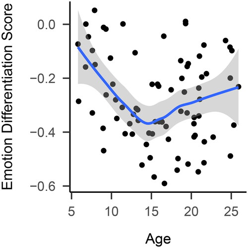
We will illustrate this using an example. Nook et al. (2018) investigated how emotion differentiation develops across the lifespan. Emotion differentiation is the ability of an individual to distinguish between different emotions, such as being angry or sad. To examine this question, Nook et al. (2018) obtained emotion differentiation scores from participants aged 4–25 years old. To make inference more challenging, we use a random subsample of size n = 80 instead of the whole sample. Figure 1 visualizes the relationship. The data are in line with the original statistical analysis, which suggests a U-shaped relationship between emotion differentiation and age, with scores falling from childhood to adolescence and increasing from adolescence to adulthood. However, the traditional tests failed to find evidence of an association, with Pearson, Kendall, and Spearman results of $t(78)=-1.59,$ p = .115; $z=-1.41,$ p = .158; and $S=98,212.00,$ p = .181; respectively.

Figure 1. Emotion differentiation across age. The blue line is a representation of the best fit obtained by using local polynomial regression fitting, and the gray area represents the corresponding 95% confidence interval.

The most common method for examining nonlinear and nonmonotonic relationships is the use of nonlinear models, such as nonlinear regression (Fox, 2016, Chapter 17). For instance, the original analysis of the emotion differentiation data set relied on a quadratic regression model. However, many nonlinear models can only capture relationships of a specific form. For example, a quadratic regression model is limited to quadratic relationships. Consequently, the appropriateness of such nonlinear models hinges on researchers having prior knowledge of the relationship type, while such knowledge is often not available. Some more general nonlinear models, like kernel regression, can capture a broader range of relationships. However, even these general models are confined to detecting mean dependence, that is, the variable Y is related to the variable X such that $E(Y)\ne E(Y|X).$ This is not the case, for example, if the variance but not the mean of Y depends on X. As a result, even general nonlinear models may not be suitable for investigating whether two variables are associated.

Hypothesis tests are available that can potentially detect any type of relationship and are thus suitable for this research question. We will call them modern¹ nonparametric independence tests. Hoeffding’s test (Hoeffding, 1948) has been available since the 1940s. Recently, the topic has gained increased attention within machine learning and nonparametric statistics. As a result, many modern nonparametric independence tests have been developed. They can be categorized into those based on ranks (Bergsma & Dassios, 2014; Chatterjee, 2021; Csörgő, 1985; Deb & Sen, 2021; Drton et al., 2020; Han et al., 2017; Heller et al., 2016; Hoeffding, 1948; Romano, 1988; Rosenblatt, 1975; Wang et al., 2017; Weihs et al., 2018), kernels (Albert et al., 2022; Gretton et al., 2008; Pfister et al., 2018), mutual information (Berrett & Samworth, 2019; Kinney & Atwal, 2014; Y. A. Reshef et al., 2016), copulas (Ding & Li, 2015; Lopez-Paz et al., 2013; Schweizer & Wolff, 1981; Zhang, 2019), pairwise distances (Heller et al., 2013; Székely et al., 2007), maximum correlation (Breiman & Friedman, 1985; Gretton et al., 2008; Papadatos & Xifara, 2013; Rényi, 1959), and U-statistics (Berrett et al., 2021).

To showcase the potential of modern nonparametric independence tests, we applied the distance correlation (Székely et al., 2007) and the Hilbert Schmidt Independence Criterion (Gretton et al., 2008), two of the most popular modern nonparametric independence tests, to the emotion differentiation example. In contrast to all traditional tests, they correctly detect that emotional differentiation and age are related: $p_{\text{dcor}}=.041,$ $p_{\text{HSIC}}=.024.$

Despite modern nonparametric independence tests having the advantage of potentially detecting any relationship, they are rarely used in psychology for several potential reasons. First, many psychological researchers are not familiarly with modern nonparametric independence tests because they are not covered in their statistical training. Second, there may be legitimate concerns about the power of the modern nonparametric independence test, especially in moderately sized samples. The disadvantage of being able to detect any relationship is that for a particular relationship the power can be reduced compared to a more specialized test. As an example, if the two variables follow a bivariate normal distribution, Pearson’s correlation typically has higher power than any modern nonparametric independence test, since it has uniformly the highest power among all unbiased tests (Lehmann & Romano, 2005, sec. 5.13). Using modern nonparametric independence tests can therefore decrease the power and be detrimental in moderately sized data sets, which are common in psychology. Fourth, the selection of the appropriate nonparametric independence test is a question that arises due to the abundance of options.

In this paper, we thus first provide an introduction to the most popular modern nonparametric independence tests for psychological researchers. In order to address power concerns and the question of which test should be used, we conducted a simulation study comparing traditional tests of independence and modern nonparametric independence tests. We included the introduced popular nonparametric tests, as well as two newly developed variants of existing tests, as candidates. The newly developed variants differentiate themselves by being specifically designed for data as they occur in psychological research, such as small sample sizes combined with weak relationships. It is not possible to identify a test that is always the most powerful, since the type of relationship determines which test has the highest power (Bergsma & Dassios, 2014; de Siqueira Santos et al., 2014; Lehmann & Romano, 2005). Previous simulation studies have consequently provided information on which tests are best for which types of relationships (de Siqueira Santos et al., 2014; Ding & Li, 2015; Kinney & Atwal, 2014; Simon et al., 2014). However, this does not resolve the question of which test should be used when the type of relationship is unknown, which is often the case in psychology. To answer this question, we establish an evaluation criterion that considers the power across all relationships, which is appropriate for answering this question.

Nonparametric independence tests

Notation

The two variables of interest are formalized as random variables X and Y. The distributions of the random variables are described by corresponding (cumulative) distribution functions $F_X(x),F_Y(y)$ and joint distribution function $F_{X,Y}(x,y).$ To reflect that the variables are continuous, the distribution functions $F_X(x),$ $F_Y(y),F_{X,Y}(x,y)$ are assumed to be continuous. Two variables are called not associated or equivalently independent if and only if $$F_{X,Y}(x,y)=F_X(x)F_Y(y).$$

To test whether the variables are independent, a sample, which consists of a series of n paired observations of X and Y is available: $\mathbf{D}=\{(x_i,y_i):i\in 1,\dots ,n\}.$ An independence test is called nonparametric if and only if its test statistic converges to 0 for independence and nonzero for any alternative,² that is, for any type of relationship between X and Y.

Selection criteria

Due to the large number of available nonparametric independence tests, we included tests according to the following criteria:

1. the availability of an R implementation;

2. the high level of popularity indicated by at least 100 citations (as of August 26, 2022, according to Google Scholar);

3. not exhibiting consistently lower power than other tests.

These criteria lead to the tests we will introduce in this section. Nonparametric independence tests that are available in R but do not meet one of the other two inclusion criteria are as follows: first, the maximal information coefficient test (D. N. Reshef et al., 2011) provided by the Minerva package (Albanese et al., 2012), which has been found to have low power compared to other tests (Gorfine et al., 2012; Kinney & Atwal, 2014; Simon et al., 2014). Second, a mutual information test using the K-nearest neighbors method (Berrett & Samworth, 2019), which is provided by the FastMIT package (Lin et al., 2019), and has not been cited 100 times. Third, the rank-based test offered in the XICOR package (Chatterjee, 2021), which has not been cited 100 times and has been demonstrated to have low power when compared to other rank-based tests (Shi et al., 2021).

Shared concepts

Before describing the tests, we introduce two concepts shared across many of them. Several tests calculate the dissimilarity between the actual joint distribution ($F_{X,Y}$) and the joint distribution assuming independence ($F_X{F}_Y$). Multiple dissimilarity measures exist such that the corresponding dissimilarity is 0 if and only if X and Y are independent. Estimates of those dissimilarities are used as test statistics for the nonparametric independence tests, with different dissimilarity measures giving rise to different tests.

Many tests use a random permutation approach to obtain the p value corresponding to the observed value of the test statistic (Good, 2005). This approach randomly permutes the values of one variable and saves the resulting test statistic t_i for each permutation i. This procedure is repeated I times to estimate a permutation sampling distribution under the null hypothesis of independence. The p value is obtained by counting the proportion of permutations for which the permutation test statistic t_i exceeds the original test statistic t.

Hoeffding’s test

Hoeffding’s test is based on the following dissimilarity measure $$\Delta (X,Y)={\int }_{-\infty }^{\infty }{\int }_{-\infty }^{\infty }{p}_{X,Y}(x,y){\left[F_{X,Y}(x,y)-F_X(x)F_Y(y)\right]}^2\hspace{0.17em}\mathit{\text{dx dy}}$$ where $p_{X,Y}(x,y)$ is the probability density function of the joint distribution. $\Delta (X,Y)$ is thus the average squared difference between the actual distribution function $F_{X,Y}(x,y)$ and the joint distribution function under independence $F_X(x)F_Y(x).$ The dissimilarity $\Delta (X,Y)$ is estimated using Hoeffding’s D. The formula for D is presented in Hollander et al. (2013, Section 8.6).

There are multiple possible approaches to obtain a p value from the observed test statistic D. One option is to rely on the combination of precalculated tables and approximate large sample distributions, as described in Hollander et al. (2013, Section 8.6). The hoeffd function included in the Hmisc package (Harrell, 2021) implements this version of Hoeffding’s test.

Distance correlation test

The distance correlation test relies on characteristic functions. The characteristic function of a random variable is the Fourier transform of its probability density function.³ If ${\phi }_X(s),{\phi }_Y(t),{\phi }_{X,Y}(s,t)$ are the characteristic functions describing the marginal distributions, and the actual joint distributions, respectively, then X and Y are independent if and only if ${\phi }_{X,Y}(x,y)={\phi }_X(x){\phi }_Y(y).$

Székely et al. (2007) proposed the following distance covariance dissimilarity measure $${\mathrm{\text{dCov}}}^2(X,Y)=\frac{1}{{\pi }^2}{\int }_{-\infty }^{\infty }{\int }_{-\infty }^{\infty }\frac{{\left|{\phi }_{X,Y}(s,t)-{\phi }_X(s){\phi }_Y(t)\right|}^2}{s^2{t}^2}\hspace{0.17em}\mathit{\text{dt ds}}.$$

The standardized version is the distance correlation: $$\mathrm{\text{dCor}}(X,Y)=\frac{{\mathrm{\text{dCov}}}^2(X,Y)}{\sqrt{\mathrm{\text{dCov}}(X,X){\mathrm{\text{dCov}}}^2(Y,Y)}},$$ which ranges between 0 (independence) and 1 (perfect dependence).

The distance correlation $\mathrm{\text{dCor}}$ is estimated via the empirical distance correlation; see Székely et al. (2007), Definition 5 for the formulas. The corresponding p value is obtained via the random permutation approach. The dcor.test function within the energy package provides an implementation of the distance correlation test.

Taustar test

The Taustar test is based on the ${\tau }^{*}$ dependence measure (Bergsma & Dassios, 2014), which is an extension of Kendall’s τ. Kendall’s τ is based on the notion of concordant and discordant pairs. A pair of observations (x₁, y₁) and (x₂, y₂) is said to be concordant if the sort order of x₁, x₂ and y₁, y₂ agrees: that is, if either both x_i > x_j and y_i > y_j holds or both x_i < x_j and y_i < y_j; otherwise they are said to be discordant.⁴ The population value for Kendall’s τ is $\tau ={\Pi }_{C_2}-{\Pi }_{D_2}$ where ${\Pi }_{C_2}$ is the probability that two observations are concordant and ${\Pi }_{D_2}$ the probability that they are discordant. If there is any monotonic relationship between X and Y, then $\tau \ne 0.$ However, τ = 0, does not imply independence for nonmonotonic relationships.

Bergsma and Dassios (2014) extended τ to ${\tau }^{*}$ such that ${\tau }^{*}=0$ implies independence for all types of relationships. The central idea is to consider concordance of quadruples (x₁, y₁), (x₂, y₂), (x₃, y₃), (x₄, y₄). A quadruple is considered concordant if it contains two pairs that are either “jointly” concordant or “jointly” discordant, while it is called discordant if, “jointly,” one pair is concordant and the other is discordant. Mathematically, a quadruple is concordant if there is a permutation $(i,j,k,l)$ of $(1,2,3,4)$ such that: $$(x_i,x_j<x_k,x_l)\wedge [(y_i,y_j<y_k,y_l)\vee (y_i,y_j>y_k,y_l)],$$ and discordant if there is a permutation $(i,j,k,l)$ such that: $$[(x_i,x_j<x_k,x_l)\vee (x_i,x_j<x_k,x_l)]\wedge [(y_i,y_k<y_j,y_l)\vee (y_i,y_k>y_j,y_l)],$$ where $\vee$ and $\wedge$ are logical OR, and AND, respectively. The population value is: $${\tau }^{*}=\frac{2{\Pi }_{C_4}-{\Pi }_{D_4}}{3},$$ where ${\Pi }_{C_4}$ is the probability that a quadruple is concordant and ${\Pi }_{D_4}$ the probability that it is discordant.

The formula for the estimate $t^{*}$ of ${\tau }^{*}$ can be found in Bergsma and Dassios (2014, Equation 5). The corresponding p value can be obtained via multiple approaches (Nandy et al., 2016), including the random permutation approach (Bergsma & Dassios, 2014), which provides the most accurate results but can be slow for large samples. The tauStarTest function within the TauStar package implements the Taustar test.

Heller-Heller-Gorfine test

The Heller-Heller-Gorfine (HHG) test (Heller et al., 2013) utilizes the following observation. Two continuous random variables X, Y are dependent if and only if dichotomizations⁵ of X and Y exist such that the resulting dichotomous variables are dependent. More specifically, the two dependent dichotomous random variables are of a specific form for whose presentation some terms need to be introduced. Let $d_X(·,·)$ and $d_Y(·,·)$ be norm-based distance metrics so that the distance between two observations x_i, x_j is $d_X(x_i,x_j),$ and the distance between two observations y_i, y_j is $d_Y(y_i,y_j).$ Furthermore, let (x₀, y₀) be a pair of x and y values, $R_{x_0},R_{y_0}$ radii around x₀ and y₀ respectively, and $I(·)$ be the indicator function. The dichotomous random variables are then of the form $I\{d_X(x_0,X)\le R_{x_0}\}$ and $I\{d_X(y_0,Y)\le R_{y_0}\}.$

As a solution to the problem that (x₀, y₀) and $R_{x_0},R_{y_0}$ are unknown, different values are employed; one set of values for each pair of observations (x_i, y_i) and (x_j, y_j) (see, Heller et al., 2013 for how this is done exactly). Nonparametric independence tests for dichotomous variables are well known, most notably the Pearson chi-squared and the likelihood ratio tests. Thus, for each dichotomization indexed by i, j, independence of the dichotomous random variables can be tested by one of those tests, with corresponding test statistic t(i, j). To combine the test results across all dichotomizations, Heller et al. (2013) propose summing across all test statistics t(i, j), such that the overall test statistic is $t={\sum }_{i=1}^n{\sum }_{\stackrel{j=1}{j\ne i}}^{n}t(i,j).$ The corresponding p value is obtained via the random permutation approach. The hhg.test function within the HHG package implements the HHG test.

In contrast to the tests discussed so far, the HHG test is not a single test but a family of tests. By choosing different distance metrics $d_X(·,·),d_Y(·,·),$ different tests are obtained. While the HHG test is consistent for all norm-based distances, the choice of the distance metric impacts the power.

Hilbert-Schmidt Independence Criterion test

The Hilbert-Schmidt Independence Criterion (HSIC) (Gretton et al., 2005) is based on the following idea. While a covariance of $\mathrm{\text{Cov}}(X,Y)=0$ does not imply independence of X and Y, $\mathrm{\text{Cov}}(f(X),g(Y))=0$ for all (bounded and continuous) transformations f, g does (Rényi, 1959). However, it is impossible to investigate all functions f, g. Gretton et al. (2005) showed that it suffices to consider all functions within the unit ball in so-called characteristic reproducing Kernel Hilbert spaces, $f\in \mathcal{F},g\in \mathcal{G}.$ This lead to the following measure of independence: $$\mathit{\text{HSIC}}=\underset{f\in \mathcal{F},g\in \mathcal{G}}{\mathrm{\text{sup}}}{\mathrm{\text{Cov}}}^2(f(X),g(Y)).$$

The kernel trick makes it possible to compute the HSIC. Only the reproducing kernels $k(x,x\prime ),l(y,y\prime )$ of the Hilbert spaces $\mathcal{G},\mathcal{F}$ respectively are needed. Put another way, instead of specifying characteristic reproducing Hilbert spaces directly, only two kernels giving rise to characteristic Hilbert spaces can be specified. Such kernels are referred to as characteristic. A popular characteristic kernel is the Gaussian kernel $k(x,x\prime )=\hspace{0.17em}\mathrm{\text{exp}}\hspace{0.17em}\left(\frac{-{(x-x\prime )}^2}{2{\sigma }^2}\right),$ with free bandwidth parameter σ. Given two characteristic kernels $k(x,x\prime ),l(y,y\prime )$ that have been centered in the sense that $E[k(x,X)]=0$ and $E[l(y,Y)]=0:$ $$\mathit{\text{HSIC}}=E[k(X,X\prime )l(Y,Y\prime )],$$ with (X, Y) and $(X\prime ,Y\prime )$ both having distribution F_XY but being independent of each other.

For a sample D, those kernels give rise to the gram matrices K, L with entries $K_{i,j}=k(x_i,x_j)$ and $L_{i,j}=l(y_i,y_j).$ The estimate of HSIC is then given by: $$\widehat{\mathrm{\text{HSIC}}}=\frac{1}{n^2}\mathrm{\text{trace}}(\mathbf{\text{KHLH}})$$ where $H=I_n-\frac{1}{n}{J}_n$ is the centering matrix, with I_n being the identity matrix of size n and J_n the n-by-n matrix of all 1s.

The p value corresponding to an estimate of HSIC can be obtained via multiple approaches (Pfister et al., 2018), including the random permutation approach, which provides the most accurate results but can be slow for large samples. The dhsic.test function within the dHSIC package implements the HSIC test.

Like the HHG test, the HSIC test is not a single test but rather a family of tests. By choosing different kernels, different tests can be implemented. In particular, by choosing the appropriate kernels, the HSIC test family contains Pearson’s correlation test (linear kernel) and the distance correlation test as special cases (see Sejdinovic et al., 2013).

New test variant: mutual information by kernel density estimation

The first new test we propose relies on the mutual information. The mutual information is a dependence measure from information theory which is 0 if and only if two variables X and Y are independent. The mutual information for continuous variables relies on probability density functions. In particular, if $p_X(x),p_y(y),p_{X,Y}(x,y)$ are the marginal and joint probability density functions, the continuous mutual information is defined as $$I(X,Y)={\int }_{-\infty }^{\infty }{\int }_{-\infty }^{\infty }{p}_{X,Y}(x,y)\hspace{0.17em}\mathrm{\text{log}}\hspace{0.17em}\left(\frac{p_{X,Y}(x,y)}{p_X(x)p_Y(y)}\right)\hspace{0.17em}\mathit{\text{dx dy}},$$

There are many approaches to estimating the continuous mutual information, most prominently, kernel density estimators (Moon et al., 1995), k-nearest neighbors (Kraskov et al., 2004), and adaptive partitioning (Steuer et al., 2002). The estimator used can have profound effects on the power of the resulting hypothesis test (Khan et al., 2007). In contrast to most existing mutual information-based tests (Berrett & Samworth, 2019; Kinney & Atwal, 2014; Y. A. Reshef et al., 2016), we chose to employ kernel density estimation since Khan et al. (2007) found that this approach worked best in samples below a size of n < 100 and high noise, which we consider to subsume most psychological data sets.

The kernel density estimator of the probability density function $p_X(x)$ is: $${\widehat{p}}_X(x)=\frac{1}{\mathit{\text{nh}}}\sum _{i=1}^{n}K\left(\frac{x-x_i}{h}\right),$$ where K is a kernel and h is the bandwidth parameter. The reproducing kernels used for the HSIC tests and the kernels here are related but different concepts. Using the kernel density estimates for the probability density functions, the mutual information can be estimated as follows: $$\widehat{I}(X,Y)=\sum _{i=1}^n{\widehat{p}}_{X,Y}(x,y)\hspace{0.17em}\mathrm{\text{log}}\hspace{0.17em}\left(\frac{{\widehat{p}}_{X,Y}(x,y)}{{\widehat{p}}_X(x){\widehat{p}}_Y(y)}\right).$$

As for the HSIC test, many options are available for the kernel and the algorithm to choose the bandwidth. We used the Epanechnikov Kernel, as it leads to the best density estimates (in the sense of minimizing the mean squared error; see, for example, Wand and Jones (1994)). We chose the Sheater-Jones plug-in algorithm for bandwidth selection, since Harpole et al. (2014) found that this algorithm outperforms all other methods. The p value corresponding to a mutual information estimate is obtained via the permutation approach. Throughout this manuscript, we will refer to this test as the mutual information by kernel density estimation (MI-KDE) test. We provide the R implementation of the MI-KDE test here: https://osf.io/yketn/ and a web application here https://solo-fsw.shinyapps.io/ModernNonparametricTests/.

New test variant: combing Pearson’s and Heller-Heller-Gorfine’s tests

The second new test combines two existing tests: the traditional test of Pearson’s correlation and the HHG test. The idea to combine these two tests emerged from the following observation: compared to other nonparametric tests, the HHG test appears to possess high power for many nonlinear relationships, but low power for linear relationships. In the comparison by de Siqueira Santos et al. (2014), it exhibited close to the highest power among the nonparametric tests investigated for all nonlinear relationships. However, it had low power for the linear relationship. Pearson’s test showed the opposite behavior. It typically had the highest power for linear relationships but tended to have low power for nonlinear relationships (de Siqueira Santos et al., 2014; Ding & Li, 2015; Kinney & Atwal, 2014; Simon et al., 2014). Thus, by combining the two tests, we aimed at a test that has relatively high power across many relationships and only slightly lower power than the HHG or Pearson tests for the relationships where those tests have the highest power. We call this test the HHG-Pearson test.

The combination is straightforward. Both tests are performed, and an overall p value is obtained by applying the Bonferroni correction. In particular, if $p_{\text{HHG}}$ and $p_{\text{Pearson}}$ are the p values of HHG’s test and Pearson’s test respectively, then the p value of the HHG-Pearson test is $p_{\text{HHG‐Pearson}}=2\mathrm{\text{min}}(p_{\text{HHG}},p_{\text{Pearson}}).$ While Bonferroni’s correction is generally conservative, it is the only formula-based correction that guarantees strong control of the family-wise error rate without additional assumptions.⁶ We provide the R implementation of the HHG-Pearson test here: https://osf.io/yketn/ and a web application here https://solo-fsw.shinyapps.io/ModernNonparametricTests/.

Comparison of tests

Tests included

We included all tests described in the previous section in the simulation study. The settings used were as recommended in the literature and are as follows. For the HHG test, we used the Euclidean distance for both $d_X(·,·)$ and $d_Y(·,·),$ along with the likelihood ratio test statistic. We chose the Euclidean distance as it was suggested in the paper introducing the HHG test and demonstrated good performance in terms of power (Heller et al., 2013). We chose the likelihood ratio test statistic, as Pearson’s test statistic is its approximation. However, this choice is likely to have only a very limited effect (Heller et al., 2013). For the HSIC test, we used the Gaussian kernel with median heuristic as bandwidth, as recommended by Pfister et al. (2018). For the distance correlation, HHG, Taustar, and MI-KDE tests, we used the random permutation approach with 1000 permutations to obtain p values. This approach was computationally infeasible for the HSIC test, so, we instead used 100 permutations. We did not employ the approximation based on eigenvalues (Gretton et al., 2009) because a preliminary investigation confirmed the findings of Pfister et al. (2018): it leads to low power.

Besides the modern nonparametric independence tests, we also included the association tests most commonly used in psychology; in particular, the traditional tests of Pearson’s, Spearman’s, and Kendall’s correlation, as implemented by the cor.test function within the stats package. Additionally, we included the permutation version of Pearson’s test. As with the other tests, we used 1000 random permutations. The code to reproduce the simulation study is available at https://osf.io/yketn/.

Design

Overview

The design of the simulation study can be summarized as follows:

1. Sample size (five levels): 10, 20, 50, 100, and 150

2. Type of relationship (six levels): mean independence, linear, inverted-U, negative exponential, cyclic, and missed moderator.

3. Strength of relationship (three levels): low, medium, high.

4. Distribution of errors (four levels): normal, skewed, heavy-tailed, heteroscedastic.

This resulted in a total of $5\times 6\times 3\times 4=360$ design cells. The details for each factor and its selected levels are described below. For all factors, we took care to select levels that are common in psychology.

Sample size

Marszalek et al. (2011) found that the most common sample sizes in psychology range from 10 to 140, while Kühberger et al. (2014) found a range from 1 to 100. Based on this, we selected five levels: 10, 20, 50, 100, 150.

Type of relationship

We visualize the included relationships in Figure 2. All relationships considered fall within the following framework: $Y=f(X)+ϵ,$ where ϵ represents the error term (see next subsection). The relationships considered were as follows: $$\begin{array}{l}\text{Mean} \text{Independence}:f(X)=0\\ \text{Linear}:f(X)=2X\\ \text{Inverted}-U:f(X)=-X^2\\ \text{Negative} \text{Exponential}:f(X)=-e^{-X}\\ \text{Cyclic}:f(X)=\text{sin}(3X)\\ \text{Missed} \text{Moderator}:f(X)=\mathit{\text{ZX}}\\ \text{with} Z\sim \text{Bernoulli}(0.5).\end{array}$$

Figure 2. Visualization of investigated relationships.

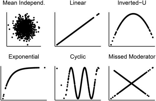
We included the linear relationships to investigate how the nonparametric independence tests perform compared to Pearson’s tests in this situation, where Pearson’s test tends to be optimal. The remaining relationships were designed to mirror common nonlinear relationships that occur in psychology. U-type relationships have been found across many domains of psychology (Grant & Schwartz, 2011), including the emotion differentiation example discussed at the beginning. Negative exponential curves are often used to model learning curves (Leibowitz et al., 2010). Cyclic patterns are commonly found in ecological momentary assessment studies (Verboon & Leontjevas, 2018). The missed moderator relationship represents a situation where the two variables are linearly related, but a third, unobserved variable moderates the relationship.

Distribution of errors

We considered a normal distribution as the baseline, as it represents the most straightforward case and is an assumption of Pearson’s correlation. Additionally, we examined skewed, heavy-tailed, and heteroscedastic error distributions, as these are frequently observed in psychological research and are known to impact Pearson’s correlation (Bishara & Hittner, 2017). For the skewed distribution, we followed Bishara and Hittner (2017) and employed a Weibull distribution with a shape parameter of 1.5 and a scale of 1, as it aptly mimics reaction times.

For the heavy-tailed errors, we used a t-distribution with six degrees of freedom. We selected six degrees of freedom because this results in substantial excess kurtosis (6), thereby robustly testing the methods’ ability to handle heavy-tailed errors while still reflecting scenarios encountered in psychological data (Blanca et al., 2013). For heteroscedastic errors, we generated the error term as $ϵ(X)=\mathit{\text{ZX}},$ where Z is a normally distributed variable with a mean of zero, as is commonly done. All error distributions were centered to have a mean of zero and were scaled to an appropriate standard deviation, contingent on the desired strength of the relationship.

Strength of relationship

To modify the strength of the relationship, we used the generalized measure of correlation (GMC) (Zheng et al., 2012), which within the setting of this study is: $$\mathit{\text{GMC}}(Y|X)=1-\frac{E[(Y-f{(X)}^2)]}{\mathrm{\text{var}}(Y)}.$$

Thus, $\mathit{\text{GMC}}(Y|X)$ denotes the amount of variance of Y that is accounted for by X. Consequently, it is the nonlinear generalization of the commonly used multiple squared correlation, the quantity adjusted R-squared estimates (Karch, 2020). Following the heuristic effect sizes proposed in the literature for R-squared (Cohen, 1988), we used the following values for $\mathit{\text{GMC}}(Y|X):$ “low”=0.1, “medium” = 0.45, “high” = 0.75. To obtain a certain GMC value, we modified the error standard deviation ${\sigma }_{ϵ}$ accordingly.

GMC is not appropriate for the missed moderator and mean independence relationship, as for both cases $\mathit{\text{GMC}}(Y|X)=0.$ For the missed moderator relationship, we used “low” = 0.3, “medium” = 0.6, “high”=1, as error standard deviations, and for mean independence, we used “low”=1, “medium”=2, “high”=4. For the mean independence condition, the error standard deviation had no impact on the results, so we will only report the results for ${\sigma }_{ϵ}=1.$

Evaluation of tests

To obtain estimates of the type I error rates and power, we generated 10,000 random samples within each cell. As significance level, we used the standard value of $\alpha =0.05.$

Type I error rates

We first examined whether a test is valid, which is the case if its type I error rate is always lower than the significance level α; that is, the actual type I error rate does not exceed the desired type I error rate. For this, we only considered cells where the null hypothesis of independence held true. This applied to all cells that exhibited mean independence and had a nonheteroscedastic error distribution.

Power

Ideally, we would want to identify the uniformly most powerful test of the valid tests (Lehmann & Romano, 2005). Unfortunately, this does not exist, as which test is most powerful depends on the type of relationship (Bergsma & Dassios, 2014). Thus, to select the test with the highest power, the type of relationship needs to be known. Such knowledge is usually not available in psychological research. Consequently, an evaluation criterion is needed that considers power across a set of relationships.

Many such criteria are available. Prominent examples are worst-case power or (weighted) average power. The former is close to the frequentist idea of minimax testing, and the latter is close to the Bayesian risk idea (Lehmann & Romano, 2005). However, which test is considered best based on these two criteria is highly dependent on the precise design of the simulation study. Consequently, the results cannot be expected to generalize well. Thus, we instead propose a criterion that is less sensitive to the design of the simulation study. It is inspired by the relationship between Student’s t test and Wilcoxon’s rank-sum test. If the t test’s assumption of normality is met, it is only slightly more powerful than Wilcoxon’s test (Hodges & Lehmann, 1956), and if it is not met, Wilcoxon’s test can be substantially more powerful (Blair & Higgins, 1980; Hodges & Lehmann, 1956). This is commonly used to argue for using Wilcoxon’s test as the default procedure instead of the t test (Posten, 1982). Similarly, we aimed to identify a test that has only slightly less power than Pearson’s test if bivariate normality is met but can have much higher power if it is not met.

Results

Type I error rates

The type I error results are shown in Table 1. Type I error rates were correctly always below 5% for almost all tests. Only Hoeffding’s test showed substantially inflated type I error rates for small and moderate sample sizes. As those sample sizes are common in psychology, we excluded Hoeffding’s test from further consideration.

Table 1. Type I error rates.

N	Error	Pear.	PearP.	Kend.	Spear.	Hoeff.	dCor	HHG	HSIC	Taustar	MI-KDE	HHG-Pear.
10	Normal	.05	.05	.05	.05	.11	.05	.05	.05	.05	.05	.04
10	Skewed	.05	.05	.05	.05	.11	.05	.05	.05	.05	.05	.05
10	Heavy	.05	.05	.05	.05	.1	.05	.05	.05	.05	.05	.04
20	Normal	.05	.05	.05	.05	.08	.05	.05	.05	.05	.05	.05
20	Skewed	.05	.05	.05	.05	.08	.05	.05	.05	.05	.05	.04
20	Heavy	.05	.05	.05	.05	.08	.05	.05	.05	.05	.05	.04
50	Normal	.05	.05	.05	.05	.06	.05	.05	.05	.05	.05	.04
50	Skewed	.05	.05	.05	.05	.06	.05	.05	.05	.05	.05	.05
50	Heavy	.05	.05	.05	.05	.06	.05	.05	.04	.05	.05	.05
100	Normal	.05	.05	.05	.05	.06	.05	.05	.05	.05	.05	.04
100	Skewed	.05	.05	.05	.05	.06	.05	.05	.05	.05	.05	.04
100	Heavy	.05	.05	.05	.05	.06	.05	.05	.05	.05	.05	.05
150	Normal	.04	.04	.04	.04	.05	.05	.05	.05	.05	.05	.04
150	Skewed	.05	.05	.05	.05	.05	.05	.05	.05	.05	.05	.04
150	Heavy	.05	.05	.05	.05	.05	.05	.05	.05	.05	.05	.05

Notes: Type I error rates are boldface if they are substantially too large (> 0.06). N = sample size. Test abbreviations: Pear.: Pearson’s; PearP.: Pearson’s permutation version; Kend.: Kendall’s; Spear.: Spearman’s; Hoeff.: Hoeffding’s; dCor: distance correlation; HHG: Heller-Heller-Gorfine; HSIC: Hilbert-Schmidt independence criterion; Taustar: Taustar; MI-KDE: mutual information via kernel density estimation; HHG-Pear.: HHG.

For all tests based on the permutation method (all tests except the traditional tests and Hoeffding’s test), these results confirm theoretical findings: permutation tests only require exchangeability to have correct type I error rates, and all included conditions meet this assumption. Indeed, exchangeability is met for any situation in which X and Y are independently and identically distributed from any joint distribution. Thus, the permutation tests have correct type I error rates for a very wide set of conditions.

Power

No test was uniformly most powerful

Table A1 in the Appendix A presents the power results for all cells. The results confirm that no test had uniformly the highest power across all cells.

The type of relationship heavily influenced which test had the highest power. Pearson’s test predominantly had the highest power⁷ for the linear (45/60 cells) and negative exponential (43/60 cells) relationships. As anticipated, all 15 cells where Pearson’s test did not exhibit the highest power for a linear relationship had nonnormal errors. In cells with heterogeneous errors, the highest power was achieved by either the HHG-Pearson or the HHG tests. This is logical, given that heterogeneous errors involve a linear dependency on both the mean—to which Pearson’s test is sensitive—and the variance—to which the HHG test is sensitive. For cells with heavy-tailed or skewed errors, Kendall’s and Spearman’s tests demonstrated the highest power, aligning with the consensus that rank-based methods are effective for these data types (Bishara & Hittner, 2017). Transitioning to the negative exponential relationship, in all 17 cells where Pearson’s test was not the most powerful, a heterogeneous error distribution was present, and the highest power was observed for either HHG, HHG-Pearson, or MI-KDE.

The proposed MI-KDE test had the highest power for the large majority of the remaining cells. Specifically, it was almost always the most powerful for the quadratic (58/60) and missed moderator relationships (58/60 cells) and predominantly had the highest power (41/60 cells) for the cyclic relationship. In the remaining 19 cells with a cyclic relationship, either the HHG or HSIC test had the highest power.

Maximum power-loss

Table 2 presents the maximum power lost across all relationships compared to Pearson’s test for each nonparametric independence test. The distance correlation and the HHG-Pearson test had a maximum power loss of around 7%, and 11%, respectively. All other tests had a power loss of at least 20%. We will therefore focus on the distance correlation and HHG-Pearson tests in the remainder of this result section.

Table 2. Maximum power lost compared to Pearson’s test.

Test	Maximum power lost
Distance correlation	.07
HHG-Pear.	.11
Taustar	.21
HHG	.34
MI-KDE	.35
HSIC	.42

Note: MI-KDE: mutual information via kernel density estimation; HHG: Heller-Heller-Gorfine; HSIC: Hilbert-Schmidt independence criterion.

Pairwise comparisons

First, we compared the two selected nonparametric tests with Pearson’s test (Figure 3). The same pattern emerged for both nonparametric tests. They typically had more power than Pearson’s test for the inverted-U, cyclic, and missed moderator relationships. Their power advantage reached as high as 93%, as shown in Table 3. In contrast, they generally had slightly less power than Pearson’s test for the negative exponential and linear relationships. However, even in these cases, the nonparametric tests often exhibited higher power when paired with heteroscedastic errors. On average, the distance correlation test was 24% more powerful, and the HHG-Pearson test was 30% more powerful.

Figure 3. Power comparisons between Pearson’s test and the distance correlation, and HHG-Pearson tests. Neg. Exp.: negative exponential; Missed Mod.: missed moderator; Mean Indep.: mean independence.

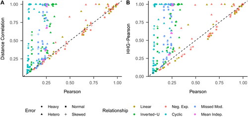
Table 3. Pairwise power comparisons.

Test1	Test2	Maximum dif.	Mean dif.	Minimum dif.
dCor	Pearson’s	.93	.24	−0.07
HHG-Pearson	Pearson’s	.93	.30	−0.11
HHG-Pearson	dCor	.53	.06	−0.07
dCor	Kendall’s	.90	.27	−0.04
dCor	Spearman’s	.91	.30	−0.03
HHG-Pearson	Kendall’s	.90	.33	−0.09
HHG-Pearson	Spearman’s	.91	.35	−0.09

Notes: Results are based on subtracting the power of Test2 from Test1. Thus, if values are positive, Test1 was more powerful. Dif. = difference.

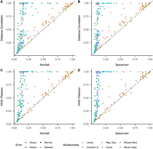
Next, we compared the two selected nonparametric tests with Spearman’s and Kendall’s rank-based tests (Figure 4). A similar pattern emerged: the nonparametric tests typically outperformed Spearman’s and Kendall’s tests in terms of power across almost all cells. For both the nonparametric tests, the maximum power advantage was 90% relative to Kendall’s test and 91% relative to Spearman’s test. The nonparametric tests exhibited only marginally lower power than either Kendall’s or Spearman’s tests in some cells. Such cells typically displayed a linear relationship, low relationship strength, and an error distribution that was not heteroscedastic (see Table A1 in the Appendix A).

Figure 4. Power comparison between Kendall’s and Spearman’s tests, and the distance correlation and HHG-Pearson tests. Neg. Exp.: negative exponential; Missed Mod.: missed moderator; Mean Indep.: mean independence.

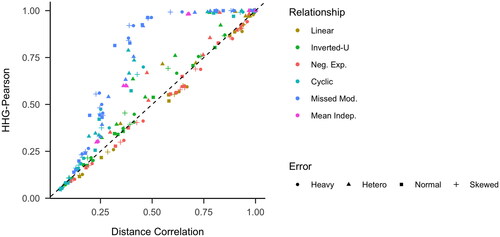
Finally, we compared the power of the HHG-Pearson and distance correlation tests (Figure 5). The HHG-Pearson test typically outperformed the distance correlation test under the following conditions: missed moderator relationships, inverted-U relationships, cyclic relationships, exponential relationships with heteroscedastic errors, and mean independence with heteroscedastic errors. Conversely, the distance correlation test generally had higher power in the cases of exponential and linear relationships, although for the latter this was only true when not paired with heteroscedastic errors. For the remaining types of relationships, the two tests exhibited roughly equal power. Notably, the HHG-Pearson test had a significant advantage, with a maximum power increase of 53%, compared to a more modest maximum advantage of 7% for the distance correlation test.

Figure 5. Power comparison between the distance correlation and HHG-Pearson tests. Neg. Exp.: negative exponential; Missed Mod.: missed moderator; Mean Indep.: mean independence.

Discussion

In this paper, we first introduced the most popular modern nonparametric independence tests, which are able to detect any relationship. We then proposed two new variants of existing nonparametric tests optimized for psychological data. Finally, we investigated which test is appropriate for deciding whether two continuous variables are associated or not, without knowledge of the type of relationship. As no test can be most powerful for all relationships, we set out to identify a test with only slightly less power than Pearson’s test in the worst case but substantially more power in many other situations.

Our central result is that for the conditions investigated the distance correlation and the Heller-Heller-Gorfine-Pearson (HHG-Pearson) tests fulfill this criterion. They both exhibited only slightly less power than Pearson’s correlation in the worst case (bivariate normal distribution), but they had significantly more power in many other situations, particularly for most nonlinear relationships.

A danger of simulation studies is that their results might not generalize beyond the conditions considered. This is especially problematic in this study, as the power of the tests considered depends heavily on the type of relationship and, to a lesser extent, the error distribution. However, we expect that this central result generalizes for the following reasons: first, we included the linear relationship with normal errors, a very favorable condition for Pearson’s correlation, and even in that case, Pearson’s test had only slightly higher power. Second, it is evident that Pearson’s test has almost zero power for some relationships and consequently substantially less power than the HHG-Pearson and distance correlation tests, whose power approaches 100% with increasing sample size for any relationship. Third, earlier simulation studies (de Siqueira Santos et al., 2014; Kinney & Atwal, 2014), which considered different types of relationships, were also unable to identify a relationship for which Pearson’s test had substantially higher power than the distance correlation test.

The distance correlation and HHG-Pearson tests were typically more powerful than Kendall’s and Spearman’s tests, with large power advantages in the best and average case and only modest power disadvantages in the worst case. While these results strongly favor the distance correlation and HHG-Pearson tests, it is important to note that we only examined one monotonic relationship and expect that there are monotonic relationships for which Kendall’s and Spearman’s tests outperform the distance correlation and HHG-Pearson tests more substantially. Nevertheless, it cannot be expected that the power advantage for those monotonic relationships is sufficiently substantial to compensate for the large power advantage distance correlation and the HHG-Pearson have for the nonmonotonic relationships we considered.

Regarding the differences between the HHG-Pearson and the distance correlation test, our results show a familiar pattern. The HHG-Pearson test had substantially more power for some conditions and only slightly less power for others, leading to a higher average power. This could constitute a reason to recommend the HHG-Pearson test. However, such a recommendation would be premature, as it may rely too heavily on the design of the simulation study. In particular, we expect that there are situations for which the distance correlation test is substantially more powerful than the HHG-Pearson test. Another argument in favor of the distance correlation test is that it was more powerful for the linear relationship (outside of heteroscedastic errors). Due to the importance of the linear relationship in psychology and the fact that the favorable properties of distance correlation have been replicated in multiple simulation studies with different designs (de Siqueira Santos et al., 2014; Ding & Li, 2015; Kinney & Atwal, 2014; Simon et al., 2014), we therefore, for now, recommend the distance correlation in favor of the HHG-Pearson test.

The newly proposed mutual information by kernel density estimation (MI-KDE) test was not selected under the chosen evaluation criterion as it did not perform well for the linear relationship. However, it was (almost) always most powerful for three out of the five relationships considered: the missed moderator, inverted-U, and cyclic relationships. Our results thus suggest that the MI-KDE test should be chosen if only those relationships are expected. Due to this favorable performance, further research comparing the MI-KDE test with other mutual information-based association tests, (Berrett & Samworth, 2019; Kinney & Atwal, 2014; Y. A. Reshef et al., 2016), is recommended.

If one expects only one certain type of relationship, arguably an approach specifically tailored for this particular relationship should be chosen. It is expected that a test specialized for a particular kind of relationship outperforms any nonparametric independence test in this case. The traditional method for doing this is to specify a statistical model that captures the desired relationship, such as a polynomial regression model. However, the findings in Edelmann and Goeman (2022) suggest that utilizing the Hilbert-Schmidt Independence Criterion (HSIC) with a kernel tailored to the anticipated associations may prove to be a more effective approach.

Besides being limited to detecting only linear relationships, another shortcoming of Pearson’s correlation is its high sensitivity to outliers, a weakness that has spurred the development of numerous robust alternatives (Wilcox, 2017). This naturally prompts the question: How robust are modern nonparametric tests? The precise robustness properties—such as breakdown points and influence functions—are unknown. Importantly, none of these tests were originally designed to be robust. The rank-based tests (Taustar, Hoeffd, and to a certain extent HHG) can be expected to be more robust than the remaining approaches relying on the raw data, as ranking of the data naturally weakens the effect of outliers. A full examination of the robustness of modern nonparametric tests is beyond the scope of this article and is recommended for future work. In the Online Supplementary, we take the first step by investigating the robustness of each test to a single outlier for two conditions. Most importantly, no test was unaffected by the single outlier. However, the rank-based tests were more robust, as expected. Consequently, we recommend using modern nonparametric tests, like the recommended distance correlation, with caution when the presence of erroneous data points cannot be excluded. Rank-based tests should provide some increased robustness to outliers (Bakker & Wicherts, 2014; Karch, 2023), and of those, especially Taustar can be recommended, as it performed best and is almost the rank-based version of the recommended distance correlation. However, future work should rigorously explore the exact robustness properties of the modern nonparametric tests and aim to develop more robust versions. A natural starting point could be the techniques used to improve the robustness of Pearson’s correlation (Wilcox, 2017).

Additional avenues for future work are as follows. First, formal mathematical comparisons of the involved tests are recommended to overcome the limited generalizability of simulation study results. In the best case, this would lead to upper limits for how much power the modern nonparametric independence tests (most prominently distance correlation) lose compared to Pearson’s tests. This might also give further insight into the relative performance of distance correlation and the HHG-Pearson test. Second, it might be possible to improve the HHG-Pearson test by replacing the Bonferroni correction with more modern approaches to combine two tests, most notably resampling-based approaches (Dudoit et al., 2008). Third, our results indicate that combining the newly proposed MI-KDE with Pearson’s test could lead to a test that performs well across many conditions. One of these two tests was the most powerful for almost all conditions investigated, yet their average power was relatively low. This suggests that they complement each other well. Fourth, after an association has been detected, quantifying its strength is usually of interest. Assuming linearity, Pearson’s correlation is the standard quantification approach. Many of the measures used as test statistics for the modern nonparametric independence tests could be used for quantification without assuming linearity. The additional challenge when using those measures for quantification is that they must be interpretable for every possible value (Reimherr & Nicolae, 2013). Unfortunately, for many measures, interpretation outside of the extremes, which denote complete dependence and complete independence, is not straightforward (Reimherr & Nicolae, 2013). Thus, more work is needed regarding the interpretation of the nonparametric independence measures.

When the selected test of independence fails to detect an association, either the variables are indeed not associated or the test incorrectly failed to detect an association. Given the large power differences among the tests, additionally applying other tests will lead to further insights. Care has to be taken, however, not to inflate type I error rates. When none of the additional tests shows a significant result, this strengthens the result and no additional action has to be performed. However, if any additional test shows a significant result, it should not be concluded that the two variables are dependent as this would risk inflating type I error rates. Instead, any significant results among the additional tests should be designated as exploratory: this is not conclusive evidence against the null hypothesis; instead, it warrants validation on a separate data set. Using scatter plots during this exploratory phase can be beneficial for exploring the type of relationship, guiding the creation of more powerful, specialized tests that must also be applied to new data to prevent overfitting. The results of our simulation study suggest that for the recommended distance correlation test, it is advisable to use Pearson’s correlation and the proposed MI-KDE test as additional tests is. One of these three tests was most powerful for 87% of the design cells. It has to be noted, however, that this result will very likely not generalize beyond the alternatives studied here.

In summary, our results indicate that if the type of relationship between two continuous variables is unknown, which is a common situation in psychological research, the distance correlation test may well be a more suitable option compared to traditional tests. The proposed HHG-Pearson test seems a promising alternative, with substantially more power in many situations. However, further investigations are needed before routine application of this test can be recommended.

Article information

Conflict of interest disclosures: Each author signed a form for disclosure of potential conflicts of interest. No authors reported any financial or other conflicts of interest in relation to the work described.

Ethical principles: The authors affirm having followed professional ethical guidelines in preparing this work. These guidelines include obtaining informed consent from human participants, maintaining ethical treatment and respect for the rights of human or animal participants, and ensuring the privacy of participants and their data, such as ensuring that individual participants cannot be identified in reported results or from publicly available original or archival data.

Funding: This work was not supported.

Role of the funders/sponsors: None of the funders or sponsors of this research had any role in the design and conduct of the study; collection, management, analysis, and interpretation of data; preparation, review, or approval of the manuscript; or decision to submit the manuscript for publication.

Acknowledgments: The ideas and opinions expressed herein are those of the authors alone, and endorsement by the authors’ institutions is not intended and should not be inferred.

Data availability statement

The code to reproduce the simulation study and its analysis can be found here: https://osf.io/yketn/.

Notes

1 We use the word “modern” to differentiate these nonparametric tests from traditional nonparametric tests, most importantly Kendall’s and Spearman’s correlation. Notably, modern nonparametric tests can detect any type of relationship, while Kendall’s and Spearman’s tests are limited to monotonic relationships.

2 Note that under this definition Kendall’s and Spearman’s test are not nonparametric.

3 This statement is only true if a probability density function exists, which is guaranteed in our setting because we assume continuous random variables.

4 Ties can be ignored, as we assume continuous distributions.

5 Dichotomization refers here to binary random variables that are functions of X and Y, respectively.

6 Holm’s procedure is a less conservative alternative but equivalent when correcting for two comparisons.

7 In precise terms, we consider a test to have the highest power if no other test exists that has higher power after rounding to two digits. This is to account for the many cells in which multiple tests had the highest power and the uncertainty in the power estimates.

Appendix A.

Detailed power results.

Table A1. Power.

Rel.	Error	N	Strength	Pear.	PearP.	Kend.	Spear.	Hoeff.	dCor	HHG	HSIC	Taustar	MI-KDE	HHG-Pear.
Linear	Heavy	10	Low	.17	.17	.15	.15	.23	.16	.09	.11	.14	.11	.13
Linear	Hetero	10	Low	.33	.32	.24	.2	.31	.35	.37	.37	.18	.39	.4
Linear	Normal	10	Low	.15	.15	.13	.13	.2	.15	.09	.09	.12	.1	.12
Linear	Skewed	10	Low	.16	.16	.14	.15	.22	.15	.09	.11	.13	.11	.12
Linear	Heavy	10	High	.95	.95	.9	.89	.9	.94	.79	.84	.84	.84	.93
Linear	Hetero	10	High	.96	.96	.96	.94	.98	.97	.95	.95	.95	.93	.97
Linear	Normal	10	High	.96	.95	.88	.88	.87	.94	.73	.79	.82	.82	.92
Linear	Skewed	10	High	.95	.95	.89	.89	.89	.94	.77	.82	.84	.84	.92
Linear	Heavy	10	Medium	.66	.66	.56	.56	.61	.63	.37	.44	.5	.45	.57
Linear	Hetero	10	Medium	.69	.68	.64	.58	.73	.71	.65	.64	.58	.62	.72
Linear	Normal	10	Medium	.63	.63	.5	.51	.55	.58	.3	.37	.44	.39	.52
Linear	Skewed	10	Medium	.64	.63	.54	.55	.6	.61	.35	.41	.48	.43	.55
Linear	Heavy	20	Low	.32	.32	.3	.31	.34	.31	.15	.18	.29	.18	.26
Linear	Hetero	20	Low	.42	.42	.36	.3	.43	.55	.74	.66	.32	.72	.72
Linear	Normal	20	Low	.28	.28	.24	.25	.27	.25	.13	.13	.22	.15	.22
Linear	Skewed	20	Low	.3	.3	.29	.3	.32	.29	.16	.17	.27	.19	.25
Linear	Heavy	20	High	1	1	1	1	1	1	.99	.99	1	1	1
Linear	Hetero	20	High	1	1	1	1	1	1	1	1	1	1	1
Linear	Normal	20	High	1	1	1	1	1	1	.98	.99	1	.99	1
Linear	Skewed	20	High	1	1	1	1	1	1	.99	.99	1	1	1
Linear	Heavy	20	Medium	.93	.93	.91	.91	.9	.93	.75	.76	.88	.8	.91
Linear	Hetero	20	Medium	.88	.88	.92	.88	.95	.95	.96	.94	.91	.93	.97
Linear	Normal	20	Medium	.93	.93	.87	.88	.86	.9	.64	.66	.83	.72	.89
Linear	Skewed	20	Medium	.93	.92	.91	.91	.91	.92	.75	.75	.88	.81	.91
Linear	Heavy	50	Low	.66	.65	.69	.69	.67	.67	.39	.4	.65	.38	.59
Linear	Hetero	50	Low	.62	.62	.66	.56	.76	.9	1	.98	.68	.98	.99
Linear	Normal	50	Low	.64	.64	.59	.59	.56	.58	.3	.29	.53	.32	.55
Linear	Skewed	50	Low	.66	.65	.68	.68	.66	.65	.41	.39	.64	.46	.6
Linear	Heavy	50	High	1	1	1	1	1	1	1	1	1	1	1
Linear	Hetero	50	High	1	1	1	1	1	1	1	1	1	1	1
Linear	Normal	50	High	1	1	1	1	1	1	1	1	1	1	1
Linear	Skewed	50	High	1	1	1	1	1	1	1	1	1	1	1
Linear	Heavy	50	Medium	1	1	1	1	1	1	1	.99	1	1	1
Linear	Hetero	50	Medium	.99	.99	1	1	1	1	1	1	1	1	1
Linear	Normal	50	Medium	1	1	1	1	1	1	.98	.97	1	.99	1
Linear	Skewed	50	Medium	1	1	1	1	1	1	1	1	1	1	1
Linear	Heavy	100	Low	.91	.91	.94	.94	.93	.94	.73	.71	.92	.64	.89
Linear	Hetero	100	Low	.81	.81	.89	.82	.97	1	1	1	.95	1	1
Linear	Normal	100	Low	.91	.91	.88	.89	.85	.88	.59	.55	.84	.56	.87
Linear	Skewed	100	Low	.91	.91	.94	.94	.93	.93	.77	.71	.92	.8	.91
Linear	Heavy	100	High	1	1	1	1	1	1	1	1	1	1	1
Linear	Hetero	100	High	1	1	1	1	1	1	1	1	1	1	1
Linear	Normal	100	High	1	1	1	1	1	1	1	1	1	1	1
Linear	Skewed	100	High	1	1	1	1	1	1	1	1	1	1	1
Linear	Heavy	100	Medium	1	1	1	1	1	1	1	1	1	1	1
Linear	Hetero	100	Medium	1	1	1	1	1	1	1	1	1	1	1
Linear	Normal	100	Medium	1	1	1	1	1	1	1	1	1	1	1
Linear	Skewed	100	Medium	1	1	1	1	1	1	1	1	1	1	1
Linear	Heavy	150	Low	.98	.98	.99	.99	.99	.99	.91	.89	.99	.82	.98
Linear	Hetero	150	Low	.9	.9	.97	.93	1	1	1	1	1	1	1
Linear	Normal	150	Low	.98	.98	.97	.97	.96	.97	.79	.74	.95	.73	.97
Linear	Skewed	150	Low	.98	.98	.99	.99	.99	.99	.94	.89	.99	.95	.98
Linear	Heavy	150	High	1	1	1	1	1	1	1	1	1	1	1
Linear	Hetero	150	High	1	1	1	1	1	1	1	1	1	1	1
Linear	Normal	150	High	1	1	1	1	1	1	1	1	1	1	1
Linear	Skewed	150	High	1	1	1	1	1	1	1	1	1	1	1
Linear	Heavy	150	Medium	1	1	1	1	1	1	1	1	1	1	1
Linear	Hetero	150	Medium	1	1	1	1	1	1	1	1	1	1	1
Linear	Normal	150	Medium	1	1	1	1	1	1	1	1	1	1	1
Linear	Skewed	150	Medium	1	1	1	1	1	1	1	1	1	1	1
Inv.-U	Heavy	10	Low	.08	.08	.06	.06	.13	.08	.07	.08	.06	.08	.07
Inv.-U	Hetero	10	Low	.23	.22	.12	.1	.19	.26	.32	.32	.09	.36	.32
Inv.-U	Normal	10	Low	.08	.08	.06	.06	.13	.08	.07	.07	.06	.08	.07
Inv.-U	Skewed	10	Low	.08	.08	.07	.07	.13	.08	.08	.08	.06	.08	.07
Inv.-U	Heavy	10	High	.26	.23	.12	.11	.28	.36	.38	.39	.13	.43	.37
Inv.-U	Hetero	10	High	.33	.29	.14	.12	.34	.47	.56	.57	.16	.61	.54
Inv.-U	Normal	10	High	.26	.23	.11	.1	.26	.33	.33	.36	.12	.4	.34
Inv.-U	Skewed	10	High	.26	.24	.13	.11	.28	.36	.38	.4	.13	.42	.37
Inv.-U	Heavy	10	Medium	.18	.16	.09	.09	.19	.21	.19	.22	.09	.23	.2
Inv.-U	Hetero	10	Medium	.27	.24	.12	.11	.23	.33	.4	.42	.11	.45	.39
Inv.-U	Normal	10	Medium	.17	.15	.08	.08	.18	.19	.16	.18	.09	.2	.17
Inv.-U	Skewed	10	Medium	.18	.17	.11	.1	.2	.21	.2	.21	.1	.23	.21
Inv.-U	Heavy	20	Low	.09	.09	.06	.06	.11	.11	.12	.11	.07	.14	.11
Inv.-U	Hetero	20	Low	.24	.24	.14	.11	.2	.41	.69	.61	.12	.69	.64
Inv.-U	Normal	20	Low	.09	.09	.06	.06	.11	.1	.1	.09	.07	.12	.1
Inv.-U	Skewed	20	Low	.09	.09	.07	.07	.12	.1	.12	.11	.07	.16	.11
Inv.-U	Heavy	20	High	.29	.28	.13	.11	.48	.72	.79	.73	.3	.86	.76
Inv.-U	Hetero	20	High	.34	.33	.15	.12	.6	.83	.94	.9	.39	.95	.92
Inv.-U	Normal	20	High	.29	.28	.12	.11	.42	.7	.74	.67	.26	.84	.71
Inv.-U	Skewed	20	High	.3	.29	.14	.11	.48	.74	.79	.73	.3	.87	.76
Inv.-U	Heavy	20	Medium	.21	.21	.1	.09	.25	.41	.44	.4	.15	.53	.41
Inv.-U	Hetero	20	Medium	.29	.29	.13	.11	.31	.61	.81	.73	.19	.82	.76
Inv.-U	Normal	20	Medium	.19	.19	.09	.08	.22	.36	.38	.34	.13	.49	.36
Inv.-U	Skewed	20	Medium	.2	.19	.11	.1	.25	.39	.43	.39	.15	.55	.39
Inv.-U	Heavy	50	Low	.09	.1	.07	.06	.13	.2	.27	.22	.11	.3	.22
Inv.-U	Hetero	50	Low	.26	.26	.15	.11	.31	.78	.99	.97	.23	.98	.99
Inv.-U	Normal	50	Low	.09	.09	.06	.06	.12	.17	.22	.17	.09	.26	.18
Inv.-U	Skewed	50	Low	.09	.09	.08	.07	.14	.19	.28	.21	.11	.39	.21
Inv.-U	Heavy	50	High	.31	.31	.14	.11	.95	1	1	.99	.92	1	1
Inv.-U	Hetero	50	High	.35	.35	.17	.13	.99	1	1	1	.99	1	1
Inv.-U	Normal	50	High	.31	.31	.14	.11	.93	.99	1	.98	.89	1	.99
Inv.-U	Skewed	50	High	.32	.31	.16	.12	.95	1	1	.99	.92	1	1
Inv.-U	Heavy	50	Medium	.24	.23	.11	.09	.61	.85	.91	.82	.52	.94	.87
Inv.-U	Hetero	50	Medium	.32	.32	.16	.12	.75	.98	1	.99	.67	1	1
Inv.-U	Normal	50	Medium	.23	.23	.1	.09	.5	.8	.85	.73	.43	.92	.8
Inv.-U	Skewed	50	Medium	.23	.23	.13	.1	.59	.85	.91	.81	.51	.96	.87
Inv.-U	Heavy	100	Low	.09	.1	.06	.06	.23	.41	.53	.42	.2	.53	.45
Inv.-U	Hetero	100	Low	.27	.27	.15	.12	.68	.99	1	1	.59	1	1
Inv.-U	Normal	100	Low	.1	.1	.06	.06	.17	.32	.43	.3	.15	.46	.34
Inv.-U	Skewed	100	Low	.09	.09	.08	.07	.23	.37	.56	.41	.2	.71	.45
Inv.-U	Heavy	100	High	.32	.32	.15	.11	1	1	1	1	1	1	1
Inv.-U	Hetero	100	High	.35	.35	.17	.13	1	1	1	1	1	1	1
Inv.-U	Normal	100	High	.32	.31	.14	.11	1	1	1	1	1	1	1
Inv.-U	Skewed	100	High	.32	.32	.17	.12	1	1	1	1	1	1	1
Inv.-U	Heavy	100	Medium	.24	.24	.11	.09	.96	1	1	.99	.95	1	1
Inv.-U	Hetero	100	Medium	.31	.31	.16	.12	1	1	1	1	.99	1	1
Inv.-U	Normal	100	Medium	.24	.23	.1	.09	.9	.99	.99	.97	.88	1	.99
Inv.-U	Skewed	100	Medium	.24	.23	.14	.11	.94	.99	1	.99	.93	1	1
Inv.-U	Heavy	150	Low	.1	.1	.07	.06	.37	.62	.75	.61	.35	.71	.67
Inv.-U	Hetero	150	Low	.27	.27	.16	.11	.96	1	1	1	.92	1	1
Inv.-U	Normal	150	Low	.1	.1	.06	.06	.27	.51	.63	.45	.25	.65	.54
Inv.-U	Skewed	150	Low	.1	.1	.08	.07	.36	.58	.78	.61	.34	.89	.69
Inv.-U	Heavy	150	High	.33	.33	.15	.12	1	1	1	1	1	1	1
Inv.-U	Hetero	150	High	.35	.35	.17	.12	1	1	1	1	1	1	1
Inv.-U	Normal	150	High	.32	.32	.14	.11	1	1	1	1	1	1	1
Inv.-U	Skewed	150	High	.32	.32	.17	.12	1	1	1	1	1	1	1
Inv.-U	Heavy	150	Medium	.24	.24	.11	.09	1	1	1	1	1	1	1
Inv.-U	Hetero	150	Medium	.32	.32	.16	.11	1	1	1	1	1	1	1
Inv.-U	Normal	150	Medium	.23	.23	.1	.09	.99	1	1	1	.99	1	1
Inv.-U	Skewed	150	Medium	.24	.24	.13	.1	1	1	1	1	1	1	1
Neg. exp.	Heavy	10	Low	.13	.13	.1	.11	.18	.12	.08	.09	.1	.09	.1
Neg. exp.	Hetero	10	Low	.28	.27	.16	.14	.23	.3	.34	.34	.12	.37	.35
Neg. exp.	Normal	10	Low	.12	.11	.08	.09	.15	.11	.07	.07	.08	.08	.09
Neg. exp.	Skewed	10	Low	.13	.13	.1	.1	.17	.12	.08	.09	.09	.09	.1
Neg. exp.	Heavy	10	High	.68	.67	.54	.53	.6	.66	.4	.45	.48	.45	.6
Neg. exp.	Hetero	10	High	.72	.71	.65	.59	.73	.75	.7	.68	.58	.68	.76
Neg. exp.	Normal	10	High	.65	.64	.49	.49	.55	.62	.35	.41	.43	.42	.56
Neg. exp.	Skewed	10	High	.66	.65	.53	.52	.59	.66	.41	.46	.48	.46	.59
Neg. exp.	Heavy	10	Medium	.38	.38	.28	.28	.36	.36	.19	.22	.25	.23	.31
Neg. exp.	Hetero	10	Medium	.46	.45	.34	.3	.43	.48	.47	.46	.28	.47	.52
Neg. exp.	Normal	10	Medium	.35	.34	.24	.24	.31	.32	.16	.19	.21	.21	.28
Neg. exp.	Skewed	10	Medium	.36	.35	.27	.27	.34	.35	.19	.21	.23	.23	.3
Neg. exp.	Heavy	20	Low	.22	.22	.17	.17	.21	.21	.11	.12	.16	.14	.18
Neg. exp.	Hetero	20	Low	.35	.34	.24	.19	.29	.47	.7	.62	.2	.68	.67
Neg. exp.	Normal	20	Low	.21	.2	.15	.15	.17	.18	.09	.1	.13	.12	.16
Neg. exp.	Skewed	20	Low	.21	.21	.17	.17	.2	.19	.12	.11	.15	.16	.17
Neg. exp.	Heavy	20	High	.92	.92	.87	.87	.88	.93	.78	.76	.85	.81	.91
Neg. exp.	Hetero	20	High	.91	.9	.92	.88	.95	.97	.98	.95	.92	.96	.98
Neg. exp.	Normal	20	High	.93	.92	.84	.84	.84	.91	.72	.69	.81	.78	.9
Neg. exp.	Skewed	20	High	.93	.93	.87	.87	.89	.93	.79	.76	.86	.82	.91
Neg. exp.	Heavy	20	Medium	.65	.65	.55	.55	.57	.65	.4	.4	.52	.48	.6
Neg. exp.	Hetero	20	Medium	.67	.67	.59	.52	.65	.78	.84	.78	.55	.82	.85
Neg. exp.	Normal	20	Medium	.63	.63	.49	.49	.5	.59	.33	.32	.44	.42	.56
Neg. exp.	Skewed	20	Medium	.64	.63	.54	.54	.57	.64	.41	.39	.51	.49	.58
Neg. exp.	Heavy	50	Low	.47	.47	.41	.4	.4	.46	.25	.23	.37	.31	.41
Neg. exp.	Hetero	50	Low	.49	.49	.41	.34	.52	.83	.99	.97	.44	.98	.99
Neg. exp.	Normal	50	Low	.45	.44	.34	.34	.32	.38	.2	.17	.3	.26	.37
Neg. exp.	Skewed	50	Low	.45	.45	.4	.4	.39	.43	.27	.22	.36	.39	.4
Neg. exp.	Heavy	50	High	1	1	1	1	1	1	1	.99	1	1	1
Neg. exp.	Hetero	50	High	1	1	1	1	1	1	1	1	1	1	1
Neg. exp.	Normal	50	High	1	1	1	1	1	1	.99	.98	1	1	1
Neg. exp.	Skewed	50	High	1	1	1	1	1	1	1	.99	1	1	1
Neg. exp.	Heavy	50	Medium	.95	.95	.93	.93	.93	.96	.85	.79	.92	.87	.94
Neg. exp.	Hetero	50	Medium	.9	.9	.91	.87	.95	.99	1	1	.93	1	1
Neg. exp.	Normal	50	Medium	.95	.95	.89	.89	.87	.93	.76	.67	.86	.83	.93
Neg. exp.	Skewed	50	Medium	.95	.95	.92	.92	.93	.96	.86	.78	.92	.92	.94
Neg. exp.	Heavy	100	Low	.72	.72	.68	.68	.67	.73	.49	.43	.66	.53	.69
Neg. exp.	Hetero	100	Low	.67	.67	.61	.53	.85	.99	1	1	.79	1	1
Neg. exp.	Normal	100	Low	.72	.71	.59	.59	.56	.65	.38	.3	.55	.47	.65
Neg. exp.	Skewed	100	Low	.73	.72	.67	.67	.66	.71	.52	.41	.65	.69	.69
Neg. exp.	Heavy	100	High	1	1	1	1	1	1	1	1	1	1	1
Neg. exp.	Hetero	100	High	1	1	1	1	1	1	1	1	1	1	1
Neg. exp.	Normal	100	High	1	1	1	1	1	1	1	1	1	1	1
Neg. exp.	Skewed	100	High	1	1	1	1	1	1	1	1	1	1	1
Neg. exp.	Heavy	100	Medium	1	1	1	1	1	1	.99	.98	1	.99	1
Neg. exp.	Hetero	100	Medium	.99	.99	1	.99	1	1	1	1	1	1	1
Neg. exp.	Normal	100	Medium	1	1	.99	.99	.99	1	.98	.94	.99	.99	1
Neg. exp.	Skewed	100	Medium	1	1	1	1	1	1	.99	.98	1	1	1
Neg. exp.	Heavy	150	Low	.87	.87	.85	.85	.84	.89	.69	.6	.83	.7	.85
Neg. exp.	Hetero	150	Low	.77	.77	.75	.67	.98	1	1	1	.97	1	1
Neg. exp.	Normal	150	Low	.87	.87	.77	.77	.74	.82	.57	.45	.73	.65	.83
Neg. exp.	Skewed	150	Low	.87	.87	.84	.83	.83	.88	.73	.59	.83	.86	.86
Neg. exp.	Heavy	150	High	1	1	1	1	1	1	1	1	1	1	1
Neg. exp.	Hetero	150	High	1	1	1	1	1	1	1	1	1	1	1
Neg. exp.	Normal	150	High	1	1	1	1	1	1	1	1	1	1	1
Neg. exp.	Skewed	150	High	1	1	1	1	1	1	1	1	1	1	1
Neg. exp.	Heavy	150	Medium	1	1	1	1	1	1	1	1	1	1	1
Neg. exp.	Hetero	150	Medium	1	1	1	1	1	1	1	1	1	1	1
Neg. exp.	Normal	150	Medium	1	1	1	1	1	1	1	.99	1	1	1
Neg. exp.	Skewed	150	Medium	1	1	1	1	1	1	1	1	1	1	1
Cyclic	Heavy	10	Low	.05	.05	.05	.06	.12	.06	.06	.07	.06	.07	.05
Cyclic	Hetero	10	Low	.2	.19	.15	.11	.27	.24	.36	.33	.13	.36	.34
Cyclic	Normal	10	Low	.05	.05	.05	.05	.12	.05	.06	.06	.05	.06	.05
Cyclic	Skewed	10	Low	.05	.05	.05	.05	.12	.06	.06	.07	.06	.06	.05
Cyclic	Heavy	10	High	.07	.07	.08	.08	.26	.13	.22	.25	.12	.27	.16
Cyclic	Hetero	10	High	.11	.11	.12	.11	.37	.19	.41	.35	.17	.38	.33
Cyclic	Normal	10	High	.08	.08	.08	.09	.25	.14	.21	.25	.13	.27	.16
Cyclic	Skewed	10	High	.07	.07	.08	.09	.26	.13	.22	.25	.12	.27	.16
Cyclic	Heavy	10	Medium	.06	.06	.07	.07	.19	.09	.12	.15	.09	.14	.09
Cyclic	Hetero	10	Medium	.15	.15	.15	.13	.36	.23	.41	.34	.17	.38	.35
Cyclic	Normal	10	Medium	.07	.06	.07	.07	.17	.09	.11	.13	.09	.13	.08
Cyclic	Skewed	10	Medium	.06	.06	.07	.07	.18	.1	.12	.14	.09	.14	.09
Cyclic	Heavy	20	Low	.05	.05	.05	.06	.1	.07	.07	.09	.07	.08	.06
Cyclic	Hetero	20	Low	.23	.22	.2	.14	.38	.39	.73	.59	.23	.66	.67
Cyclic	Normal	20	Low	.05	.05	.05	.05	.1	.06	.07	.08	.06	.07	.05
Cyclic	Skewed	20	Low	.05	.05	.05	.06	.1	.07	.08	.09	.07	.09	.06
Cyclic	Heavy	20	High	.06	.06	.11	.1	.43	.25	.61	.48	.26	.51	.47
Cyclic	Hetero	20	High	.11	.11	.17	.13	.63	.38	.87	.63	.39	.66	.79
Cyclic	Normal	20	High	.06	.06	.1	.1	.4	.24	.55	.46	.24	.51	.42
Cyclic	Skewed	20	High	.06	.06	.1	.1	.42	.25	.58	.48	.25	.5	.45
Cyclic	Heavy	20	Medium	.05	.05	.08	.08	.24	.16	.27	.29	.16	.3	.18
Cyclic	Hetero	20	Medium	.17	.17	.21	.15	.56	.41	.81	.63	.36	.68	.74
Cyclic	Normal	20	Medium	.05	.05	.07	.07	.21	.13	.22	.25	.14	.26	.15
Cyclic	Skewed	20	Medium	.06	.06	.08	.08	.23	.14	.26	.27	.15	.29	.18
Cyclic	Heavy	50	Low	.05	.05	.06	.06	.13	.1	.15	.17	.11	.17	.11
Cyclic	Hetero	50	Low	.23	.23	.33	.19	.75	.77	1	.97	.57	.98	.99
Cyclic	Normal	50	Low	.05	.05	.06	.06	.11	.08	.12	.13	.09	.14	.08
Cyclic	Skewed	50	Low	.05	.05	.06	.06	.13	.1	.16	.16	.1	.19	.11
Cyclic	Heavy	50	High	.06	.06	.16	.14	.95	.81	1	.93	.84	.94	.99
Cyclic	Hetero	50	High	.12	.12	.3	.2	1	.93	1	.98	.97	.98	1
Cyclic	Normal	50	High	.06	.06	.15	.14	.93	.8	.99	.92	.81	.94	.99
Cyclic	Skewed	50	High	.06	.06	.15	.14	.95	.8	1	.93	.83	.95	.99
Cyclic	Heavy	50	Medium	.06	.06	.12	.12	.57	.46	.8	.72	.46	.79	.7
Cyclic	Hetero	50	Medium	.17	.17	.37	.23	.97	.89	1	.98	.89	.98	1
Cyclic	Normal	50	Medium	.06	.06	.11	.11	.48	.4	.7	.63	.39	.74	.57
Cyclic	Skewed	50	Medium	.06	.06	.11	.11	.54	.43	.78	.69	.43	.78	.66
Cyclic	Heavy	100	Low	.05	.05	.07	.07	.2	.17	.31	.32	.18	.36	.21
Cyclic	Hetero	100	Low	.24	.24	.48	.25	.99	.99	1	1	.96	1	1
Cyclic	Normal	100	Low	.05	.05	.07	.07	.16	.14	.22	.22	.15	.29	.15
Cyclic	Skewed	100	Low	.05	.05	.08	.08	.21	.16	.32	.31	.19	.45	.22
Cyclic	Heavy	100	High	.07	.07	.24	.22	1	1	1	1	1	1	1
Cyclic	Hetero	100	High	.14	.14	.48	.31	1	1	1	1	1	1	1
Cyclic	Normal	100	High	.07	.07	.24	.22	1	1	1	1	1	1	1
Cyclic	Skewed	100	High	.07	.07	.24	.22	1	1	1	1	1	1	1
Cyclic	Heavy	100	Medium	.07	.06	.16	.16	.97	.94	1	.98	.94	1	.99
Cyclic	Hetero	100	Medium	.18	.18	.57	.34	1	1	1	1	1	1	1
Cyclic	Normal	100	Medium	.07	.07	.16	.15	.92	.89	.99	.95	.87	.99	.97
Cyclic	Skewed	100	Medium	.06	.06	.15	.15	.96	.93	1	.98	.93	1	.99
Cyclic	Heavy	150	Low	.06	.06	.1	.1	.32	.29	.49	.5	.3	.56	.38
Cyclic	Hetero	150	Low	.24	.24	.62	.33	1	1	1	1	1	1	1
Cyclic	Normal	150	Low	.05	.05	.08	.08	.24	.22	.35	.34	.23	.47	.26
Cyclic	Skewed	150	Low	.06	.05	.08	.08	.3	.26	.5	.48	.28	.71	.38
Cyclic	Heavy	150	High	.09	.09	.31	.28	1	1	1	1	1	1	1
Cyclic	Hetero	150	High	.14	.14	.6	.39	1	1	1	1	1	1	1
Cyclic	Normal	150	High	.08	.08	.3	.28	1	1	1	1	1	1	1
Cyclic	Skewed	150	High	.08	.08	.32	.29	1	1	1	1	1	1	1
Cyclic	Heavy	150	Medium	.07	.07	.22	.21	1	1	1	1	1	1	1
Cyclic	Hetero	150	Medium	.19	.19	.72	.43	1	1	1	1	1	1	1
Cyclic	Normal	150	Medium	.07	.07	.2	.19	1	1	1	1	1	1	1
Cyclic	Skewed	150	Medium	.07	.07	.21	.2	1	1	1	1	1	1	1
Mis. mod.	Heavy	10	Low	.15	.14	.1	.09	.15	.13	.14	.14	.07	.17	.15
Mis. mod.	Hetero	10	Low	.22	.21	.13	.11	.19	.25	.33	.33	.09	.37	.33
Mis. mod.	Normal	10	Low	.14	.14	.09	.08	.14	.12	.12	.12	.07	.15	.14
Mis. mod.	Skewed	10	Low	.14	.14	.1	.09	.15	.12	.13	.13	.07	.16	.14
Mis. mod.	Heavy	10	High	.24	.23	.16	.13	.22	.26	.51	.44	.11	.52	.45
Mis. mod.	Hetero	10	High	.24	.23	.16	.12	.24	.29	.61	.5	.12	.58	.54
Mis. mod.	Normal	10	High	.24	.23	.16	.13	.22	.26	.48	.43	.11	.51	.43
Mis. mod.	Skewed	10	High	.24	.23	.16	.13	.23	.26	.49	.43	.11	.52	.44
Mis. mod.	Heavy	10	Medium	.19	.19	.13	.11	.18	.19	.27	.26	.09	.31	.27
Mis. mod.	Hetero	10	Medium	.24	.22	.14	.11	.21	.26	.42	.38	.1	.43	.39
Mis. mod.	Normal	10	Medium	.19	.19	.12	.11	.17	.18	.23	.23	.09	.29	.24
Mis. mod.	Skewed	10	Medium	.19	.18	.12	.1	.17	.18	.25	.24	.08	.3	.25
Mis. mod.	Heavy	20	Low	.16	.16	.11	.09	.14	.16	.25	.22	.08	.35	.24
Mis. mod.	Hetero	20	Low	.24	.24	.14	.11	.19	.37	.7	.6	.12	.68	.63
Mis. mod.	Normal	20	Low	.16	.16	.1	.09	.12	.15	.2	.18	.08	.31	.2
Mis. mod.	Skewed	20	Low	.16	.16	.11	.09	.13	.16	.25	.21	.08	.36	.23
Mis. mod.	Heavy	20	High	.24	.23	.18	.12	.25	.39	.9	.8	.15	.96	.85
Mis. mod.	Hetero	20	High	.26	.26	.19	.13	.29	.46	.95	.86	.17	.97	.92
Mis. mod.	Normal	20	High	.24	.24	.17	.13	.24	.39	.88	.79	.15	.96	.83
Mis. mod.	Skewed	20	High	.24	.24	.17	.12	.24	.39	.89	.79	.14	.96	.84
Mis. mod.	Heavy	20	Medium	.2	.2	.14	.11	.17	.26	.57	.49	.11	.69	.5
Mis. mod.	Hetero	20	Medium	.25	.25	.16	.12	.22	.41	.81	.71	.13	.81	.75
Mis. mod.	Normal	20	Medium	.2	.2	.13	.11	.16	.25	.5	.43	.1	.65	.44
Mis. mod.	Skewed	20	Medium	.2	.2	.14	.11	.17	.25	.55	.46	.1	.67	.48
Mis. mod.	Heavy	50	Low	.17	.17	.12	.09	.14	.24	.64	.52	.1	.76	.56
Mis. mod.	Hetero	50	Low	.26	.25	.16	.12	.26	.71	.99	.97	.19	.98	.99
Mis. mod.	Normal	50	Low	.16	.16	.11	.09	.12	.2	.52	.38	.09	.67	.44
Mis. mod.	Skewed	50	Low	.17	.17	.12	.09	.14	.23	.64	.51	.1	.79	.56
Mis. mod.	Heavy	50	High	.25	.24	.2	.13	.48	.81	1	1	.32	1	1
Mis. mod.	Hetero	50	High	.26	.25	.2	.13	.65	.89	1	1	.41	1	1
Mis. mod.	Normal	50	High	.24	.24	.19	.13	.43	.8	1	1	.3	1	1
Mis. mod.	Skewed	50	High	.25	.25	.2	.13	.46	.81	1	1	.32	1	1
Mis. mod.	Heavy	50	Medium	.21	.21	.16	.11	.23	.5	.98	.94	.17	.99	.96
Mis. mod.	Hetero	50	Medium	.26	.26	.17	.12	.34	.78	1	.99	.23	1	1
Mis. mod.	Normal	50	Medium	.21	.21	.16	.11	.2	.45	.96	.89	.15	.99	.92
Mis. mod.	Skewed	50	Medium	.21	.21	.15	.12	.22	.48	.97	.92	.16	.99	.96
Mis. mod.	Heavy	100	Low	.17	.16	.12	.1	.17	.41	.95	.88	.14	.97	.92
Mis. mod.	Hetero	100	Low	.25	.24	.15	.11	.55	.98	1	1	.42	1	1
Mis. mod.	Normal	100	Low	.17	.17	.11	.09	.14	.32	.87	.72	.11	.93	.81
Mis. mod.	Skewed	100	Low	.16	.16	.11	.09	.16	.39	.95	.86	.13	.98	.92
Mis. mod.	Heavy	100	High	.24	.24	.2	.13	.99	1	1	1	.94	1	1
Mis. mod.	Hetero	100	High	.26	.26	.21	.14	1	1	1	1	1	1	1
Mis. mod.	Normal	100	High	.25	.25	.2	.13	.97	1	1	1	.9	1	1
Mis. mod.	Skewed	100	High	.25	.24	.2	.13	.99	1	1	1	.92	1	1
Mis. mod.	Heavy	100	Medium	.22	.22	.16	.12	.43	.9	1	1	.34	1	1
Mis. mod.	Hetero	100	Medium	.25	.25	.17	.12	.82	1	1	1	.65	1	1
Mis. mod.	Normal	100	Medium	.21	.21	.15	.11	.32	.84	1	1	.27	1	1
Mis. mod.	Skewed	100	Medium	.22	.21	.16	.11	.39	.88	1	1	.32	1	1
Mis. mod.	Heavy	150	Low	.18	.17	.12	.1	.23	.64	1	.98	.2	1	.99
Mis. mod.	Hetero	150	Low	.26	.26	.16	.12	.92	1	1	1	.83	1	1
Mis. mod.	Normal	150	Low	.16	.16	.11	.09	.17	.48	.98	.9	.14	.99	.96
Mis. mod.	Skewed	150	Low	.16	.16	.12	.09	.21	.59	1	.98	.18	1	.99
Mis. mod.	Heavy	150	High	.24	.24	.2	.13	1	1	1	1	1	1	1
Mis. mod.	Hetero	150	High	.25	.25	.2	.13	1	1	1	1	1	1	1
Mis. mod.	Normal	150	High	.25	.25	.2	.13	1	1	1	1	1	1	1
Mis. mod.	Skewed	150	High	.24	.24	.21	.13	1	1	1	1	1	1	1
Mis. mod.	Heavy	150	Medium	.21	.21	.16	.12	.76	1	1	1	.68	1	1
Mis. mod.	Hetero	150	Medium	.25	.25	.17	.12	1	1	1	1	.99	1	1
Mis. mod.	Normal	150	Medium	.21	.21	.15	.11	.58	.99	1	1	.52	1	1
Mis. mod.	Skewed	150	Medium	.21	.21	.16	.11	.72	.99	1	1	.63	1	1
Mean Indep.	Hetero	10	Low	.23	.21	.12	.1	.18	.24	.3	.31	.09	.35	.3
Mean Indep.	Hetero	10	High	.21	.2	.12	.1	.18	.23	.3	.31	.09	.34	.3
Mean Indep.	Hetero	10	Medium	.22	.2	.12	.1	.18	.23	.3	.31	.08	.34	.3
Mean Indep.	Hetero	20	Low	.25	.25	.14	.11	.19	.38	.65	.57	.11	.65	.6
Mean Indep.	Hetero	20	High	.24	.24	.13	.1	.18	.36	.65	.57	.11	.65	.6
Mean Indep.	Hetero	20	Medium	.24	.24	.13	.11	.18	.37	.65	.57	.11	.66	.6
Mean Indep.	Hetero	50	Low	.25	.25	.14	.11	.24	.68	.99	.96	.17	.97	.98
Mean Indep.	Hetero	50	High	.25	.25	.15	.11	.23	.67	.99	.95	.18	.97	.98
Mean Indep.	Hetero	50	Medium	.26	.26	.15	.11	.24	.68	.99	.96	.17	.97	.98
Mean Indep.	Hetero	100	Low	.26	.26	.15	.11	.46	.97	1	1	.36	1	1
Mean Indep.	Hetero	100	High	.25	.25	.16	.11	.47	.97	1	1	.37	1	1
Mean Indep.	Hetero	100	Medium	.26	.25	.14	.1	.48	.97	1	1	.37	1	1
Mean Indep.	Hetero	150	Low	.25	.25	.15	.11	.85	1	1	1	.75	1	1
Mean Indep.	Hetero	150	High	.25	.25	.15	.11	.84	1	1	1	.73	1	1
Mean Indep.	Hetero	150	Medium	.25	.25	.15	.11	.84	1	1	1	.74	1	1

Notes: Bold numbers highlight the highest power within each row (not considering Hoeffding’s test due to inflated type I error rates). If multiple numbers are boldface, multiple tests had the highest power. N: sample size; Rel.: type of relationship; Test abbreviations: Pear.: Pearson’s; PearP.: Pearson’s permutation version; Kend.: Kendall’s; Spear.: Spearman’s; Hoeff.: Hoeffding’s; dCor: distance correlation; HHG: Heller-Heller-Gorfine; HSIC: Hilbert-Schmidt independence criterion; Taustar: Taustar; MI-KDE: mutual information via kernel density estimation; HHG-Pear.: HHG.

References

- Albanese, D., Filosi, M., Visintainer, R., Riccadonna, S., Jurman, G., & Furlanello, C. (2012). Minerva and minepy: A C engine for the MINE suite and its R, Python and MATLAB wrappers. Bioinformatics, 29(3), 407–408. https://doi.org/10.1093/bioinformatics/bts707
- Albert, M., Laurent, B., Marrel, A., & Meynaoui, A. (2022). Adaptive test of independence based on HSIC measures. The Annals of Statistics, 50(2), 858–879. https://doi.org/10.1214/21-AOS2129
- Bakker, M., & Wicherts, J. M. (2014). Outlier removal, sum scores, and the inflation of the type i error rate in independent samples t tests: The power of alternatives and recommendations. Psychological Methods, 19(3), 409–427. https://doi.org/10.1037/met0000014
- Bergsma, W., & Dassios, A. (2014). A consistent test of independence based on a sign covariance related to Kendall’s tau. Bernoulli, 20(2), 1006–1028. https://doi.org/10.3150/13-BEJ514
- Berrett, T. B., Kontoyiannis, I., & Samworth, R. J. (2021). Optimal rates for independence testing via u-statistic permutation tests. The Annals of Statistics, 49(5), 2457–2490. https://doi.org/10.1214/20-AOS2041
- Berrett, T. B., & Samworth, R. J. (2019). Nonparametric independence testing via mutual information. Biometrika, 106(3), 547–566. https://doi.org/10.1093/biomet/asz024
- Bishara, A. J., & Hittner, J. B. (2017). Confidence intervals for correlations when data are not normal. Behavior Research Methods, 49(1), 294–309. https://doi.org/10.3758/s13428-016-0702-8
- Blair, R. C., & Higgins, J. J. (1980). The power of t and Wilcoxon statistics: A comparison. Evaluation Review, 4(5), 645–656. https://doi.org/10.1177/0193841X8000400506
- Blanca, M. J., Arnau, J., López-Montiel, D., Bono, R., & Bendayan, R. (2013). Skewness and kurtosis in real data samples. Methodology, 9(2), 78–84. https://doi.org/10.1027/1614-2241/a000057
- Breiman, L., & Friedman, J. H. (1985). Estimating optimal transformations for multiple regression and correlation. Journal of the American Statistical Association, 80(391), 580–598. https://doi.org/10.1080/01621459.1985.10478157
- Chatterjee, S. (2021). A new coefficient of correlation. Journal of the American Statistical Association, 116(536), 2009–2022. https://doi.org/10.1080/01621459.2020.1758115
- Cohen, J. (1988). Statistical power analysis for the behavioral sciences (2nd ed). L. Erlbaum Associates.
- Csörgő, S. (1985). Testing for independence by the empirical characteristic function. Journal of Multivariate Analysis, 16(3), 290–299. https://doi.org/10.1016/0047-259X(85)90022-3
- Deb, N., & Sen, B. (2021). Multivariate rank-based distribution-free nonparametric testing using measure transportation. Journal of the American Statistical Association, 118(541), 192–207. https://doi.org/10.1080/01621459.2021.1923508
- de Siqueira Santos, S., Takahashi, D. Y., Nakata, A., & Fujita, A. (2014). A comparative study of statistical methods used to identify dependencies between gene expression signals. Briefings in Bioinformatics, 15(6), 906–918. https://doi.org/10.1093/bib/bbt051
- Ding, A. A., & Li, Y. (2015). Copula correlation: An equitable dependence measure and extension of Pearson’s correlation. http://arxiv.org/abs/1312.7214
- Drton, M., Han, F., & Shi, H. (2020). High-dimensional consistent independence testing with maxima of rank correlations. The Annals of Statistics, 48(6), 3206–3227. https://doi.org/10.1214/19-AOS1926
- Dudoit, S., Van Der Laan, M. J., & van Der Laan, M. J. (2008). Multiple testing procedures with applications to genomics. Springer.
- Edelmann, D., & Goeman, J. (2022). A regression perspective on generalized distance covariance and the Hilbert–Schmidt independence criterion. Statistical Science, 37(4), 562–579. https://doi.org/10.1214/21-STS841
- Fox, J. (2016). Applied regression analysis and generalized linear models (3rd ed.). Sage.
- Good, P. (2005). Permutation, parametric and bootstrap tests of hypotheses (3rd ed). Springer.
- Gorfine, M., Heller, R., & Heller, Y. (2012). Comment on “detecting novel associations in large data sets.” http://www.math.tau.ac.il/∼ruheller/Papers/science6.pdf
- Grant, A. M., & Schwartz, B. (2011). Too much of a good thing: The challenge and opportunity of the inverted U. Perspectives on Psychological Science: A Journal of the Association for Psychological Science, 6(1), 61–76. https://doi.org/10.1177/1745691610393523
- Gretton, A., Bousquet, O., Smola, A., & Schölkopf, B. (2005). Measuring statistical dependence with Hilbert-Schmidt norms. In S. Jain, H. U. Simon, & E. Tomita (Eds.), Algorithmic learning theory (pp. 63–77). Springer. https://doi.org/10.1007/11564089_7
- Gretton, A., Fukumizu, K., Harchaoui, Z., & Sriperumbudur, B. K. (2009). A fast, consistent kernel two-sample test. In Y. Bengio, D. Schuurmans, J. Lafferty, C. Williams, & A. Culotta (Eds.), Advances in neural information processing systems (Vol. 22). Curran Associates, Inc. https://proceedings.neurips.cc/paper_files/paper/2009/file/9246444d94f081e3549803b928260f56-Paper.pdf
- Gretton, A., Fukumizu, K., Teo, C. H., Song, L., Schölkopf, B., & Smola, A. J. (2008). A kernel statistical test of independence. In J. C. Platt, D. Koller, Y. Singer, & S. T. Roweis (Eds.), Advances in neural information processing systems (Vol. 20, pp. 585–592). Curran Associates. http://papers.nips.cc/paper/3201-a-kernel-statistical-test-of-independence.pdf
- Gretton, A., Herbrich, R., Smola, A., Bousquet, O., & Schölkopf, B. (2005). Kernel Methods for Measuring Independence. Journal of Machine Learning Research, 6(70), 2075–2129.
- Guastello, S. J., Koopmans, M., & Pincus, D. (Eds.). (2008). Chaos and complexity in psychology: The theory of nonlinear dynamical systems. Cambridge University Press. https://doi.org/10.1017/CBO9781139058544
- Han, F., Chen, S., & Liu, H. (2017). Distribution-free tests of independence in high dimensions. Biometrika, 104(4), 813–828. https://doi.org/10.1093/biomet/asx050
- Harpole, J. K., Woods, C. M., Rodebaugh, T. L., Levinson, C. A., & Lenze, E. J. (2014). How bandwidth selection algorithms impact exploratory data analysis using kernel density estimation. Psychological Methods, 19(3), 428–443. https://doi.org/10.1037/a0036850
- Harrell, F. E., Jr. (2021). Hmisc: Harrell miscellaneous [Manual]. https://CRAN.R-project.org/package=Hmisc
- Heller, R., Heller, Y., & Gorfine, M. (2013). A consistent multivariate test of association based on ranks of distances. Biometrika, 100(2), 503–510. https://doi.org/10.1093/biomet/ass070
- Heller, R., Heller, Y., Kaufman, S., Brill, B., & Gorfine, M. (2016). Consistent distribution-free k-sample and independence tests for univariate random variables. The Journal of Machine Learning Research, 17(1), 978–1031.
- Hodges, J. L., & Lehmann, E. L. (1956). The efficiency of some nonparametric competitors of the $t$-test. The Annals of Mathematical Statistics, 27(2), 324–335. https://www.jstor.org/stable/2236996 https://doi.org/10.1214/aoms/1177728261
- Hoeffding, W. (1948). A non-parametric test of independence. The Annals of Mathematical Statistics, 19(4), 546–557. https://www.jstor.org/stable/2236021 https://doi.org/10.1214/aoms/1177730150
- Hollander, M., Wolfe, D. A., & Chicken, E. (2013). Nonparametric statistical methods. John Wiley & Sons.
- Karch, J. D. (2020). Improving on adjusted R-squared. Collabra: Psychology, 6(1), 1–11. https://doi.org/10.1525/collabra.343
- Karch, J. D. (2023). Outliers may not be automatically removed. Journal of Experimental Psychology: General, 152(6), 1735–1753. https://doi.org/10.1037/xge0001357
- Kendall, M. G. (1938). A new measure of rank correlation. Biometrika, 30(1-2), 81–93. https://doi.org/10.2307/2332226
- Khan, S., Bandyopadhyay, S., Ganguly, A. R., Saigal, S., Erickson, D. J., Protopopescu, V., & Ostrouchov, G. (2007). Relative performance of mutual information estimation methods for quantifying the dependence among short and noisy data. Physical Review. E, Statistical, Nonlinear, and Soft Matter Physics, 76(2 Pt 2), 026209. https://doi.org/10.1103/PhysRevE.76.026209
- Kinney, J. B., & Atwal, G. S. (2014). Equitability, mutual information, and the maximal information coefficient. Proceedings of the National Academy of Sciences, 111(9), 3354–3359. https://doi.org/10.1073/pnas.1309933111
- Kraskov, A., Stögbauer, H., & Grassberger, P. (2004). Estimating mutual information. Physical Review. E, Statistical, Nonlinear, and Soft Matter Physics, 69(6 Pt 2), 066138. https://doi.org/10.1103/PhysRevE.69.066138
- Kühberger, A., Fritz, A., & Scherndl, T. (2014). Publication bias in psychology: A diagnosis based on the correlation between effect size and sample size. PLoS One, 9(9), e105825. https://doi.org/10.1371/journal.pone.0105825
- Lehmann, E. L., & Romano, J. P. (2005). Testing statistical hypotheses (3rd ed.). Springer.
- Leibowitz, N., Baum, B., Enden, G., & Karniel, A. (2010). The exponential learning equation as a function of successful trials results in sigmoid performance. Journal of Mathematical Psychology, 54(3), 338–340. https://doi.org/10.1016/j.jmp.2010.01.006
- Lin, S., Zhu, J., Pan, W., & Wang, X. (2019). Fastmit: Fast mutual information based independence test [Manual]. https://CRAN.R-project.org/package=fastmit
- Lopez-Paz, D., Hennig, P., & Schölkopf, B. (2013). The randomized dependence coefficient. http://arxiv.org/abs/1304.7717
- Marszalek, J. M., Barber, C., Kohlhart, J., & Holmes, C. B. (2011). Sample size in psychological research over the past 30 years. Perceptual and Motor Skills, 112(2), 331–348. https://doi.org/10.2466/03.11.PMS.112.2.331-348
- Moon, Y.-I., Rajagopalan, B., & Lall, U. (1995). Estimation of mutual information using kernel density estimators. Physical Review. E, Statistical Physics, Plasmas, Fluids, and Related Interdisciplinary Topics, 52(3), 2318–2321. https://doi.org/10.1103/PhysRevE.52.2318
- Nandy, P., Weihs, L., & Drton, M. (2016). Large-sample theory for the Bergsma-Dassios sign covariance. Electronic Journal of Statistics, 10(2), 2287–2311. https://doi.org/10.1214/16-EJS1166
- Nook, E. C., Sasse, S. F., Lambert, H. K., McLaughlin, K. A., & Somerville, L. H. (2018). The nonlinear development of emotion differentiation: Granular emotional experience is low in adolescence. Psychological Science, 29(8), 1346–1357. https://doi.org/10.1177/0956797618773357
- Papadatos, N., & Xifara, T. (2013). A simple method for obtaining the maximal correlation coefficient and related characterizations. Journal of Multivariate Analysis, 118, 102–114. https://doi.org/10.1016/j.jmva.2013.03.017
- Pfister, N., Bühlmann, P., Schölkopf, B., & Peters, J. (2018). Kernel-based tests for joint independence. Journal of the Royal Statistical Society Series B: Statistical Methodology, 80(1), 5–31. https://ideas.repec.org/a/bla/jorssb/v80y2018i1p5-31.html https://doi.org/10.1111/rssb.12235
- Posten, H. O. (1982). Two-sample Wilcoxon power over the Pearson system and comparison with the t -test. Journal of Statistical Computation and Simulation, 16(1), 1–18. https://doi.org/10.1080/00949658208810602
- Reimherr, M., & Nicolae, D. L. (2013). On quantifying dependence: A framework for developing interpretable measures. Statistical Science, 28(1), 116–130. https://doi.org/10.1214/12-STS405
- Rényi, A. (1959). On measures of dependence. Acta Mathematica Academiae Scientiarum Hungarica, 10(3), 441–451. https://doi.org/10.1007/BF02024507
- Reshef, D. N., Reshef, Y. A., Finucane, H. K., Grossman, S. R., McVean, G., Turnbaugh, P. J., Lander, E. S., Mitzenmacher, M., & Sabeti, P. C. (2011). Detecting novel associations in large data sets. Science, 334(6062), 1518–1524. https://doi.org/10.1126/science.1205438
- Reshef, Y. A., Reshef, D. N., Finucane, H. K., Sabeti, P. C., & Mitzenmacher, M. (2016). Measuring dependence powerfully and equitably. The Journal of Machine Learning Research, 17(1), 7406–7468.
- Romano, J. P. (1988). A bootstrap revival of some nonparametric distance tests. Journal of the American Statistical Association, 83(403), 698–708. https://doi.org/10.2307/2289293
- Rosenblatt, M. (1975). A quadratic measure of deviation of two-dimensional density estimates and a test of independence. The Annals of Statistics, 3(1), 1–14. https://www.jstor.org/stable/2958076 https://doi.org/10.1214/aos/1176342996
- Schweizer, B., & Wolff, E. F. (1981). On nonparametric measures of dependence for random variables. The Annals of Statistics, 9(4), 879–885. https://doi.org/10.1214/aos/1176345528
- Sejdinovic, D., Sriperumbudur, B., Gretton, A., & Fukumizu, K. (2013). Equivalence of distance-based and RKHS-based statistics in hypothesis testing. The Annals of Statistics, 41(5), 2263–2291. https://doi.org/10.1214/13-AOS1140
- Shi, H., Drton, M., & Han, F. (2021). On the power of Chatterjee rank correlation. http://arxiv.org/abs/2008.11619
- Simon, N., & Tibshirani, R. (2014). Comment on “detecting novel associations in large data sets” by Reshef Et Al, Science Dec 16, 2011. http://arxiv.org/abs/1401.7645
- Steuer, R., Kurths, J., Daub, C. O., Weise, J., & Selbig, J. (2002). The mutual information: Detecting and evaluating dependencies between variables. Bioinformatics, 18(suppl_2), S231–S240. https://doi.org/10.1093/bioinformatics/18.suppl_2.S231
- Székely, G. J., Rizzo, M. L., & Bakirov, N. K. (2007). Measuring and testing dependence by correlation of distances. The Annals of Statistics, 35(6), 2769–2794. https://doi.org/10.1214/009053607000000505
- Verboon, P., & Leontjevas, R. (2018). Analyzing cyclic patterns in psychological data: A tutorial. The Quantitative Methods for Psychology, 14(4), 218–234. https://doi.org/10.20982/tqmp.14.4.p218
- Wand, M. P., & Jones, M. C. (1994). Kernel smoothing. CRC Press.
- Wang, X., Jiang, B., & Liu, J. S. (2017). Generalized R-squared for detecting dependence. Biometrika, 104(1), 129–139. https://doi.org/10.1093/biomet/asw071
- Weihs, L., Drton, M., & Meinshausen, N. (2018). Symmetric rank covariances: A generalized framework for nonparametric measures of dependence. Biometrika, 105(3), 547–562. https://doi.org/10.1093/biomet/asy021
- Wilcox, R. (2017). Modern statistics for the social and behavioral sciences: A practical introduction. CRC Press.
- Zhang, K. (2019). BET on independence. Journal of the American Statistical Association, 114(528), 1620–1637. https://doi.org/10.1080/01621459.2018.1537921
- Zheng, S., Shi, N.-Z., & Zhang, Z. (2012). Generalized measures of correlation for asymmetry, nonlinearity, and beyond. Journal of the American Statistical Association, 107(499), 1239–1252. https://doi.org/10.1080/01621459.2012.710509