Parametric g-formula for Testing Time-Varying Causal Effects: What It Is, Why It Matters, and How to Implement It in Lavaan

Abstract

Psychologists leverage longitudinal designs to examine the causal effects of a focal predictor (i.e., treatment or exposure) over time. But causal inference of naturally observed time-varying treatments is complicated by treatment-dependent confounding in which earlier treatments affect confounders of later treatments. In this tutorial article, we introduce psychologists to an established solution to this problem from the causal inference literature: the parametric g-computation formula. We explain why the g-formula is effective at handling treatment-dependent confounding. We demonstrate that the parametric g-formula is conceptually intuitive, easy to implement, and well-suited for psychological research. We first clarify that the parametric g-formula essentially utilizes a series of statistical models to estimate the joint distribution of all post-treatment variables. These statistical models can be readily specified as standard multiple linear regression functions. We leverage this insight to implement the parametric g-formula using lavaan, a widely adopted R package for structural equation modeling. Moreover, we describe how the parametric g-formula may be used to estimate a marginal structural model whose causal parameters parsimoniously encode time-varying treatment effects. We hope this accessible introduction to the parametric g-formula will equip psychologists with an analytic tool to address their causal inquiries using longitudinal data.

Keywords:

• Causal inference
• longitudinal data
• propensity scores
• post-treatment confounding
• time-varying confounding

Psychological researchers often seek to examine how the causal impact of a focal predictor (i.e., treatment or exposure) unfolds over time. For example, researchers might be interested in examining how maternal employment affects children’s cognitive development (Kühhirt & Klein, 2018), or how bullying at work affects sickness absences (Mathisen et al., 2022), or how poverty affects depression (Thomson et al., 2022), or how loneliness affects depressive symptoms (VanderWeele et al., 2011). In these examples, naturally observed treatments cannot merely be assumed to be one-off occurrences, but are rather continuous or successive. Importantly, treatments are time-varying: Treatments fluctuate, accumulate, or evolve over time.

Drawing valid causal conclusions about time-varying treatments from observational studies is a well-recognized challenge; see, e.g., Bray et al. (2006) and VanderWeele et al. (2016). As discussed extensively in the biostatistics and epidemiology literatures, causal inferences about time-varying treatments are exceedingly problematic because of the existence of time-varying confounders that are inevitably affected by earlier treatments (Daniel et al., 2013). Such treatment-dependent confounding variables result in causal feedback between the treatments and confounders over time (Daniel, 2018; Hernán & Robins, 2020). Under such settings, standard analytic methods for confounding adjustment fail, leading to incorrect causal conclusions (Keogh et al., 2017; Moodie & Stephens, 2010; Rosenbaum, 1984).

An approach to resolve treatment-dependent confounding is the parametric g-computation formula, colloquially termed the g-formula (Robins, 1986). The g-formula belongs to the established family of causal methods for generalized treatments (so-called “g-methods”) developed in pioneering work by James Robins and colleagues to address time-varying confounding when testing the effects of a time-varying treatment. The effectiveness of the g-computation formula is established in the causal inference methodological literature outside of psychology, notably in epidemiology and (bio)statistics; see, e.g., Naimi et al. (2016) and Hernán and Robins (2020). The g-formula has been widely implemented by applied researchers pursuing answers to causal questions in public health and the medical sciences. A few selected examples include Danaei et al. (2013), Edwards et al. (2014), Keil et al. (2014), Taubman et al. (2009) and Westreich et al. (2012), among many others.

In this article, we introduce the parametric g-computation formula, or simply g-formula, to the psychological literature. We have organized the remainder of the article following a “causal roadmap” (Ahern, 2018; Hernán, 2018) over four sections. First, we will explain the salient causal assumptions encoded in the underlying data-generating mechanism. Second, we will define the time-varying causal effects of interest; i.e., causal estimands. Third, we will introduce the g-formula for estimating the treatment effects over time. As we will explain below, the core of the parametric g-formula lies in a series of statistical models to estimate the joint distribution of all post-treatment variables (except treatment itself) that may be caused by at least one treatment instance. Hence, these statistical models can be readily specified as standard multiple linear regression functions, which are familiar to psychological researchers. Fourth, we will present the estimation procedure. To make the parametric g-formula accessible to a broad audience of psychological researchers, we implement the parametric g-formula using lavaan (Rosseel, 2012), a widely adopted structural equation modeling package in R (R Core Team, 2021).¹ Table 1 provides a glossary of key causal inferential terms used in this article. Throughout this article, we use a real-world study in psychological science as a running example. To ease the exposition and to provide intuitive explanations for applied researchers, we include a series of boxes to “annotate” each step of the g-formula. All R scripts implementing the procedure are freely available online (https://github.com/wwloh/gformula-lavaan).

Table 1. Glossary of key terms used in this paper.

Term	Description
Confounder	A variable that induces a “spurious” (or noncausal) association between a treatment and an outcome when unadjusted for.
Collider	A variable on a noncausal path with two arrows pointing at it. We emphasize that a collider is not a variable-specific role but a path-specific role. That is, a variable that is a collider on one path can be a noncollider on a different path, with both paths having the same endpoints.
Treatment-dependent confounder	A variable that simultaneously is a confounder of a later treatment on the outcome and is itself affected by an earlier or past treatment. It is also variously termed a time-varying, time-dependent, treatment-induced, or post-treatment confounder.
Propensity score	The conditional probability that an individual would have selected treatment given their pretreatment covariates.
G-computation formula, or g-formula	Links a marginal potential outcome (i.e., target causal quantity) to the average observed outcome conditional on all causally preceding variables, weighted by the probability distribution of the time-varying covariates under hypothetically fixed treatment levels.
Marginal structural model (MSM)	A model for the distribution (often expectation) of a single potential outcome in terms of parameters encoding causal effects of treatment. It is marginal because it does not model the joint distribution of different potential outcomes (such as their correlations), and it is structural because it is a potential outcomes model whose coefficients are endowed with a causal interpretation.
Doubly robust estimator	An estimator that combines: (i) a propensity score model for the treatment conditional on pretreatment covariates, and (ii) an outcome model conditional on the treatment and the pretreatment covariates. A doubly robust estimator is protected from biases due to incorrectly specifying one of these models if the other model is correctly specified.

Causal assumptions

To situate the discussion of causal assumptions, we will use a running example from psychological research. The example is based on a real-world study: the Flint Adolescent Study. This longitudinal study, beginning in 1994, followed ninth graders from four public high schools in Flint, Michigan (Zimmerman, 2014). For the purpose of illustration, we will use data from three study waves (hereafter timepoints t = 1, 2, 3) to investigate whether loneliness can undermine friendship quality over time. Both variables were repeatedly recorded in each timepoint. Further study details are provided in Appendix A. For ease of presentation, we will ignore the hierarchical structure of the data (students are nested in classrooms and schools) in our presentation, but will briefly consider clustering in Appendix A. Below, we focus on two key causal assumptions for g-formula using the example: the causal structure inducing treatment-dependent confounding, and the sequential ignorability assumption.

Causal structure inducing treatment-dependent confounding

Investigating the effect of a nonrandomized treatment (e.g., loneliness) requires thinking carefully about confounders. When assessing time-varying causal effects, in addition to stable baseline covariates (whose values remain constant throughout the study), we need to consider confounders that can vary over time during the course of the study. In our running example, one such confounder could be students’ family support (L). Family support can protect against loneliness and is likely correlated with friendship quality due to hidden common causes. Crucially, family support can change over time and is likely affected by earlier feelings of loneliness, making it a treatment-dependent confounder whose levels need to be recorded at each measurement timepoint. Although there are likely multiple time-varying confounders, to ease the exposition we will consider family support as the only confounder.

The assumed causal structure of our data-generating mechanism can be readily visualized in Figure 1 as a causal diagram (Greenland et al., 1999; Pearl, 2009; Spirtes et al., 2001).² As the causal diagram shows, three variables were repeatedly measured at each timepoint: loneliness (binary treatment or exposure X), the student’s friendship quality (continuous outcome Y), and their family support (continuous treatment-dependent confounder L). Throughout this paper, we assume that all post-treatment variables, such as the time-varying confounder L and outcome Y, are continuous. Subscripts index the timepoint t that a variable is recorded. Hence, we let X_t, L_t, and Y_t denote the treatment, treatment-dependent confounder, and outcome at each timepoint t, respectively. To simplify discussions of causal diagrams in this paper, we will consider different measurements of the same variable, such as L₁ and L₂, as distinct variables shown as different nodes (Hernán & Robins, 2020; Pearl, 2009). Note that within each survey at timepoint t, L_t and Y_t are assumed to influence X_t causally. Of importance, L_t is likely to be affected by the earlier treatment $X_{t-1}.$ In Figure 1, this causal feedback between treatment and confounder is depicted by the arrows from L₂ to X₂, and from X₁ to L₂, respectively. Because L₂ is also associated with Y₃, it is thus a confounder of the $X_2\to Y_3$ relation, while simultaneously being affected by the earlier treatment X₁ (hence the term “treatment-dependent confounder”). For the same reasons, the intermediate outcome Y₂ also plays the role of a treatment-dependent confounder of the $X_2\to Y_3$ relation. Because both L_t and Y_t are measured contemporaneously at the same survey timepoint t, we follow Daniel et al. (2013) and leave their causal relationship unspecified and merely allow for correlated errors induced by the unmeasured common cause(s) U_t specific to each timepoint t. The node U represents a (set of) hidden or unmeasured time-invariant common cause(s) of U_t that induces correlations among L and Y. Finally, for simplicity, we denote time-invariant covariates measured at baseline (age, gender, race, and family socioeconomic status in our running example) collectively by C. More complete descriptions of the variables and a snapshot of the observed data are provided in Appendix A.

Figure 1. Causal diagram for the running example across three timepoints with a treatment-dependent confounder (family support; L) and a repeatedly-measured outcome (friendship quality; Y). Notes: A circular node, such as U, denotes a (set of) unmeasured variable(s). For visual clarity, arrows emanating from unmeasured nodes are drawn in grey, whereas the causal paths corresponding to the treatment effects are drawn as dashed arrows. Descriptions of the treatment effects are provided in the main text. As is common in most longitudinal designs, at the last timepoint (e.g., t = 3) only the outcome is utilized in the analysis to allow time for the causal effect of treatment on the outcome to transpire (Gollob & Reichardt, 1987). For visual simplicity, edges emanating from the baseline time-invariant covariate(s) C to all observed time-varying variables are reduced and truncated in the causal diagram.

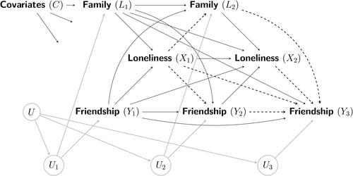
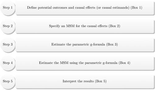
Figure 2. Implementing the parametric g-formula in five steps.

Sequential ignorability assumption

Throughout this paper, we will maintain the sequential ignorability assumption (also termed no unmeasured confounding) that, when there is no causal effect, the treatment and outcome are conditionally independent given a set of pretreatment covariates (Hernán & Robins, 2020; Imbens & Rubin, 2015; Morgan & Winship, 2015; Pearl, 2009). In our running example depicted in Figure 1, an adjustment set of measured covariates that is sufficient to block all noncausal paths between X₁ and either Y₂ or Y₃ is ${\mathcal{C}}_1=(C,L_1,Y_1).$ That is, among individuals with the same values of the variables $C,L_1,$ and Y₁, loneliness at time 1 (X₁) will be independent of friendship quality at both times 2 (Y₂) and 3 (Y₃) in the absence of a causal effect of X₁. Similarly, the causal effect of X₂ on Y₃ is unconfounded given the sufficient adjustment set ${\mathcal{C}}_2=(C,L_1,Y_1,X_1,L_2,Y_2).$ Note that the pretreatment covariates in each adjustment set temporally (and causally) precede the treatment at each focal timepoint separately. We will use the term “pretreatment” to refer to the observed history preceding treatment at a specific time, and the term “baseline” to refer to stable variables whose values remain constant throughout the study (i.e., time-invariant). For example, the adjustment set ${\mathcal{C}}_2$ contains the baseline covariate(s) C, time-varying covariate L₂ and outcome Y₂. Note that L₂ and Y₂ occur after the first treatment instance X₁. We emphasize that under the causal diagram in Figure 1, it is unnecessary to include (unmeasured) U and U_t in the adjustment sets for sequential ignorability to hold because the other measured covariates in ${\mathcal{C}}_1$ and ${\mathcal{C}}_2$ suffice to block all noncausal paths from the treatments X₁ and X₂, respectively, to the outcomes. However, this condition relies on U and U_t being unassociated with the time-varying treatments X_t. We elaborate on this assumption in the context of unobserved stable traits in the Discussion section.

Causal estimands describing time-varying treatment effects

In this section, we define the time-varying causal effects of interest. We also explain why treatment-dependent confounding precludes consistent estimation of these effects jointly using standard regression methods.

We define causal effects in terms of population-level average or expected potential outcomes. A potential outcome is the outcome that would have been observed, potentially counter to fact, had treatment been hypothetically manipulated and fixed at specific levels. To define the potential outcomes, we first explain what such a hypothetical treatment sequence entails. As a probative example, consider a hypothetical scenario where everyone receives treatment in the first timepoint $(X_1=1)$ but not in the second timepoint $(X_2=0).$ In other words, we will suppose that researchers could hypothetically manipulate each individual’s loneliness to be fixed, possibly contrary to actual conditions, at the levels $X_1=1$ (lonely) and $X_2=0$ (not lonely). Following the notation in Daniel (2018), we express such a hypothetical manipulation as “$(X_1,X_2)\leftarrow (1,0),$” where the arrow emphasizes that X₁ and X₂ are uniformly fixed at specific levels of treatment, here 1 and 0, respectively. These hypothetical manipulations can be interpreted in terms of Pearl’s (2009) “do-operator;” Gische et al. (2021) provide a detailed illustration of interventions arising from the do-operator in which the level of X is fixed at specific values.

We can then define the expected potential outcome under this counterfactual scenario. For example, the expected potential outcome for Y₂ at t = 2 is expressed as: (1) $${\mathrm{E}}_{(X_1,X_2)\leftarrow (1,0)}(Y_2);$$(1) where $\mathrm{E}()$ is the expectation operator. The expected potential outcome for Y₃ at t = 3 is similarly expressed as: (2) $${\mathrm{E}}_{(X_1,X_2)\leftarrow (1,0)}(Y_3).$$(2)

Causal effects, henceforth termed causal estimands, can then be defined by the differences between average potential outcomes following different sequences of hypothetical treatments. For example, interest may be in comparing the difference in average potential outcomes under two distinct hypothetical manipulations: one in which everyone is treated only at timepoint 1 or $(X_1,X_2)\leftarrow (1,0),$ and the other in which no one is treated at both timepoints or $(X_1,X_2)\leftarrow (0,0).$ The causal effect of X₁ on Y₂ corresponding to this difference in average potential outcomes for Y₂ can then be defined as: (3) $${\mathrm{E}}_{(X_1,X_2)\leftarrow (1,0)}(Y_2)-{\mathrm{E}}_{(X_1,X_2)\leftarrow (0,0)}(Y_2).$$(3)

Similarly, the lag-2 causal effect of X₁ on Y₃, with treatment at the second (intermediate) timepoint fixed at zero (i.e., $X_2=0$), is: (4) $${\mathrm{E}}_{(X_1,X_2)\leftarrow (1,0)}(Y_3)-{\mathrm{E}}_{(X_1,X_2)\leftarrow (0,0)}(Y_3).$$(4)

The causal effect of X₂ on Y₃, with $X_1=1$ in the earlier timepoint, would entail the difference: (5) $${\mathrm{E}}_{(X_1,X_2)\leftarrow (1,1)}(Y_3)-{\mathrm{E}}_{(X_1,X_2)\leftarrow (1,0)}(Y_3).$$(5)

Using standard path tracing rules (Pearl, 2009; Wright, 1934) in the causal diagram in Figure 1, the causal effect of X₂ on Y₃ is the path-specific effect along the $X_2\to Y_3$ causal path, whereas the causal effect of X₁ on Y₃ is the combination of path-specific effects of X₁ on Y₃ along the causal paths that do not intersect X₂; i.e., $X_1\to L_2\to Y_3,X_1\to Y_2\to Y_3,$ and $X_1\to Y_3.$ Dashed arrows indicate the causal paths corresponding to these treatment effects in Figure 1.

Box 1 Causal effects for the running example.

Does loneliness affect relationship quality over time? To answer this question, we analyzed data from the Flint Adolescent Study. As a probative example, we will examine whether individuals’ friendship quality at the end of the study (t = 3) was affected by loneliness at the earlier timepoints (t = 1 and t = 2). This causal inquiry can be answered using the following causal effects:

• (a) the effect of loneliness at t = 1 on end-of-study friendship quality (t = 3); and

• (b) the effect of loneliness at t = 2 on end-of-study friendship quality (t = 3).

How do we define these causal effects using average potential outcomes? We will start with the more straightforward effect: the lag-1 effect in (b). This effect in (b) can be defined as the difference between the following average potential outcomes:

• (b0) the average potential friendship quality at t = 3 if individuals, possibly counter to fact, did not feel lonely at t = 2; and

• (b1) the average potential friendship quality at t = 3 if individuals, possibly counter to fact, felt lonely at t = 2.

In other words, the causal effect in (b) is obtained by calculating the distinct average potential outcomes (b0) and (b1) separately and then taking their difference. This causal effect, or causal estimand, is mathematically expressed in the main text as Equation (5)(5) $${\mathrm{E}}_{(X_1,X_2)\leftarrow (1,1)}(Y_3)-{\mathrm{E}}_{(X_1,X_2)\leftarrow (1,0)}(Y_3).$$(5) .

We now turn to the effect in (a). This effect is similarly defined as the difference between two average potential outcomes. However, because this is a lag-2 effect, it necessitates considering what the loneliness level at the intermediate timepoint (t = 2) should be. For simplicity, suppose our interest is in the effect of loneliness initially at t = 1 without feeling lonely at t = 2. Then, the causal effect in (a) can be defined as the difference between the following average potential outcomes:

• (a0) the average potential friendship quality at t = 3 if individuals, possibly counter to fact, did not feel lonely at both t = 1 and t = 2; and

• (a1) the average potential friendship quality at t = 3 if individuals, possibly counter to fact, felt lonely at t = 1 but not at t = 2.

In other words, the causal effect in (a) is obtained by calculating the distinct average potential outcomes (a0) and (a1) separately, and then taking their difference. This causal estimand is mathematically expressed in the main text as Equation (4)(4) $${\mathrm{E}}_{(X_1,X_2)\leftarrow (1,0)}(Y_3)-{\mathrm{E}}_{(X_1,X_2)\leftarrow (0,0)}(Y_3).$$(4) .

How the g-formula resolves the challenge of treatment-dependent confounding

In this section, we briefly explain why treatment-dependent confounding rules out consistently estimating the causal effects of X₁ and X₂ on Y₃ using standard regression methods. Intuitively, one may consider estimating these causal effects jointly simply by regressing Y₃ on both X₁ and X₂ while adjusting for confounders. But should we adjust for the time-varying variables L₂ and Y₂? To answer this question, we inspect the causal diagram in Figure 1, focusing on L₂. We can see that L₂ is simultaneously: (i) a collider on the noncausal path $X_1\to L_2\leftarrow U_2\leftarrow U\to U_3\to Y_3;$ (ii) an intervening (i.e., intermediate) variable on the causal path $X_1\to L_2\to Y_3;$ and (iii) a confounder of X₂ and Y₃ on the noncausal path $X_2\leftarrow L_2\to Y_3.$ Hence, in a regression of Y₃ on both X₁ and X₂, adjusting for L₂ would eliminate confounding bias in the effect of X₂, but introduce so-called “collider(-stratification) bias” (Elwert & Winship, 2014; Griffith et al., 2020) and “over-adjustment bias” (Schisterman et al., 2009) in the effect of X₁. A description of how collider bias along a noncausal path can be generated is provided in the glossary in Table 1. A detailed causal diagrammatic examination of how collider and over-adjustment biases can arise simultaneously (and possibly be mitigated) in common longitudinal designs is provided in Loh and Ren (2023c). The same argument applies when adjusting for the intermediate outcome Y₂. In other words, valid inference of the effects of X₁ and X₂ on Y₃ jointly using standard regression methods is impossible because it necessitates simultaneously adjusting for and not adjusting for L₂ and Y₂.³

In contrast, the g-formula resolves this problem by decoupling adjusting, and not adjusting, for treatment-dependent confounders such as L₂ and Y₂. As we will explain in the next section, the g-formula simultaneously avoids confounding bias in the effect of X₂ and Y₃ (by first adjusting for L₂ and Y₂), and avoids collider and over-adjustment biases in the effect of X₁ and Y₃ (by subsequently marginalizing or averaging over the counterfactual distribution of L₂ and Y₂ so that they are not adjusted for). Therefore, under the sequential ignorability assumption, causal estimands obtained using the g-formula can be bestowed with a causal interpretation.

Introducing the g-formula

The g-formula starts with the joint probability distribution of the observed variables $(C,L_1,Y_1,X_1,L_2,Y_2,X_2,Y_3)$ in the naturally occurring longitudinal data. In particular, the joint probability can be factorized into a product of conditional probabilities based on the data-generating process depicted in a causal diagram (Pearl, 2009; Shpitser & Pearl, 2006; Spirtes et al., 2001). Longitudinal designs have the strength that they imply certain temporal-logical constraints, so that each variable can be conditioned on all variables temporally and causally preceding it. Therefore, we can use the causal structure in  Figure 1 to guide how we factorize the joint distribution. For notational brevity, we denote the conditional probability of A given B by $\mathrm{p}(a|b)\equiv \mathrm{p}(A=a|B=b),$ where uppercase letters denote random variables, and lowercase letters denote specific values.

Following the causal diagram in Figure 1, the joint probability can be factorized as: (6) $$\begin{array}{l}\mathrm{p}(C=c,L_1=l_1,Y_1=y_1,X_1=x_1,L_2=l_2,Y_2=y_2,X_2=x_2,Y_3=y_3)=\mathrm{p}(c,l_1,y_1)\mathrm{p}(x_1|l_1,y_1,c)\mathrm{p}(l_2,y_2|x_1,l_1,y_1,c)\mathrm{p}(x_2|l_2,y_2,x_1,l_1,y_1,c)\hspace{1em}\times \mathrm{p}(y_3|x_2,l_2,y_2,x_1,l_1,y_1,c).\end{array}$$(6)

Each element in Equation (6)(6) $$\begin{array}{l}\mathrm{p}(C=c,L_1=l_1,Y_1=y_1,X_1=x_1,L_2=l_2,Y_2=y_2,X_2=x_2,Y_3=y_3)=\mathrm{p}(c,l_1,y_1)\mathrm{p}(x_1|l_1,y_1,c)\mathrm{p}(l_2,y_2|x_1,l_1,y_1,c)\mathrm{p}(x_2|l_2,y_2,x_1,l_1,y_1,c)\hspace{1em}\times \mathrm{p}(y_3|x_2,l_2,y_2,x_1,l_1,y_1,c).\end{array}$$(6) describes the conditional probability of a variable given the variables causally preceding it. For example, $\mathrm{p}(y_3|x_2,l_2,y_2,x_1,l_1,y_1,c)$ describes the conditional probability of the outcome Y₃ at the final timepoint t = 3, given all variables in the earlier timepoints. Similarly, $\mathrm{p}(l_2,y_2|x_1,l_1,y_1,c)$ describes the conditional joint probability of the time-varying covariate L₂ and outcome Y₂ at timepoint t = 2, given the variables $X_1,L_1,Y_1,$ and C in the earlier timepoint. The joint probability of the pretreatment variables $C,L_1,$ and Y₁ preceding the first treatment instance X₁ is denoted by $\mathrm{p}(c,l_1,y_1).$

For the observed outcome at t = 2, its expectation can be computed using the joint probability in Equation (6)(6) $$\begin{array}{l}\mathrm{p}(C=c,L_1=l_1,Y_1=y_1,X_1=x_1,L_2=l_2,Y_2=y_2,X_2=x_2,Y_3=y_3)=\mathrm{p}(c,l_1,y_1)\mathrm{p}(x_1|l_1,y_1,c)\mathrm{p}(l_2,y_2|x_1,l_1,y_1,c)\mathrm{p}(x_2|l_2,y_2,x_1,l_1,y_1,c)\hspace{1em}\times \mathrm{p}(y_3|x_2,l_2,y_2,x_1,l_1,y_1,c).\end{array}$$(6) as: (7) $$\begin{array}{l}\mathrm{E}(Y_2)=\sum _{y_2}{y}_2\mathrm{p}(y_2)\\ =\sum _{y_2}{y}_2\left\{\sum _{c,l_1,y_1,x_1}\mathrm{p}(c,l_1,y_1,x_1,y_2)\right\}\\ =\sum _{c,l_1,y_1,x_1}\sum _{y_2}{y}_2\mathrm{p}(y_2|x_1,l_1,y_1,c)\mathrm{p}(c,l_1,y_1)\mathrm{p}(x_1|l_1,y_1,c)\\ =\sum _{c,l_1,y_1,x_1}\mathrm{E}(Y_2|x_1,l_1,y_1,c)\mathrm{p}(c,l_1,y_1)\mathrm{p}(x_1|l_1,y_1,c).\end{array}$$(7)

The first and fourth equalities follow the definition of an expectation operator,⁴ and the second and third equalities follow the law of total probability using the factorization in Equation (6)(6) $$\begin{array}{l}\mathrm{p}(C=c,L_1=l_1,Y_1=y_1,X_1=x_1,L_2=l_2,Y_2=y_2,X_2=x_2,Y_3=y_3)=\mathrm{p}(c,l_1,y_1)\mathrm{p}(x_1|l_1,y_1,c)\mathrm{p}(l_2,y_2|x_1,l_1,y_1,c)\mathrm{p}(x_2|l_2,y_2,x_1,l_1,y_1,c)\hspace{1em}\times \mathrm{p}(y_3|x_2,l_2,y_2,x_1,l_1,y_1,c).\end{array}$$(6) (Pearl et al., 2016, chapter 1). Similarly, the expected observed outcome at t = 3 is: (8) $$\begin{array}{l}\mathrm{E}(Y_3)=\sum _{c,l_1,y_1,x_1,l_2,y_2,x_2}\mathrm{E}(Y_3|x_2,l_2,y_2,x_1,l_1,y_1,c)\\ \hspace{1em}\times \mathrm{p}(c,l_1,y_1)\mathrm{p}(x_1|l_1,y_1,c)\mathrm{p}(l_2,y_2|x_1,l_1,y_1,c)\mathrm{p}(x_2|l_2,y_2,x_1,l_1,y_1,c).\end{array}$$(8)

However, the joint probability distribution in Equation (6)(6) $$\begin{array}{l}\mathrm{p}(C=c,L_1=l_1,Y_1=y_1,X_1=x_1,L_2=l_2,Y_2=y_2,X_2=x_2,Y_3=y_3)=\mathrm{p}(c,l_1,y_1)\mathrm{p}(x_1|l_1,y_1,c)\mathrm{p}(l_2,y_2|x_1,l_1,y_1,c)\mathrm{p}(x_2|l_2,y_2,x_1,l_1,y_1,c)\hspace{1em}\times \mathrm{p}(y_3|x_2,l_2,y_2,x_1,l_1,y_1,c).\end{array}$$(6) and expected outcomes in Equations (7)(7) $$\begin{array}{l}\mathrm{E}(Y_2)=\sum _{y_2}{y}_2\mathrm{p}(y_2)\\ =\sum _{y_2}{y}_2\left\{\sum _{c,l_1,y_1,x_1}\mathrm{p}(c,l_1,y_1,x_1,y_2)\right\}\\ =\sum _{c,l_1,y_1,x_1}\sum _{y_2}{y}_2\mathrm{p}(y_2|x_1,l_1,y_1,c)\mathrm{p}(c,l_1,y_1)\mathrm{p}(x_1|l_1,y_1,c)\\ =\sum _{c,l_1,y_1,x_1}\mathrm{E}(Y_2|x_1,l_1,y_1,c)\mathrm{p}(c,l_1,y_1)\mathrm{p}(x_1|l_1,y_1,c).\end{array}$$(7) and (8)(8) $$\begin{array}{l}\mathrm{E}(Y_3)=\sum _{c,l_1,y_1,x_1,l_2,y_2,x_2}\mathrm{E}(Y_3|x_2,l_2,y_2,x_1,l_1,y_1,c)\\ \hspace{1em}\times \mathrm{p}(c,l_1,y_1)\mathrm{p}(x_1|l_1,y_1,c)\mathrm{p}(l_2,y_2|x_1,l_1,y_1,c)\mathrm{p}(x_2|l_2,y_2,x_1,l_1,y_1,c).\end{array}$$(8) pertain only to the naturally observed data. The fundamental goal of a causal inquiry is to ascertain what would have happened to the joint probability (and the expected implied potential outcome) if treatment at each time was hypothetically fixed to a specific value, possibly counter to actuality. We initially focus on the counterfactual scenario $(X_1,X_2)\leftarrow (1,0);$ i.e., everyone received treatment in the first timepoint $(X_1=1)$ but not in the second timepoint $(X_2=0).$ To formulate this counterfactual scenario, we can imagine altering Equation (6)(6) $$\begin{array}{l}\mathrm{p}(C=c,L_1=l_1,Y_1=y_1,X_1=x_1,L_2=l_2,Y_2=y_2,X_2=x_2,Y_3=y_3)=\mathrm{p}(c,l_1,y_1)\mathrm{p}(x_1|l_1,y_1,c)\mathrm{p}(l_2,y_2|x_1,l_1,y_1,c)\mathrm{p}(x_2|l_2,y_2,x_1,l_1,y_1,c)\hspace{1em}\times \mathrm{p}(y_3|x_2,l_2,y_2,x_1,l_1,y_1,c).\end{array}$$(6) by replacing the stochastic conditional probabilities of the observed treatment at each timepoint, $\mathrm{p}(x_1|l_1,y_1,c)$ and $\mathrm{p}(x_2|l_2,y_2,x_1,l_1,y_1,c),$ with indicator functions, $\mathbb{1}\mathrm{}({\mathit{X}}_1=1)$ and $\mathbb{1}\mathrm{}({\mathit{X}}_2=0),$ respectively, where $\mathbb{1}\mathrm{}(\mathit{A})$ equals one if event A is true, and zero otherwise.⁵ The counterfactual joint probability distribution under this alteration (i.e., hypothetical manipulation) would then be: (9) $$\begin{array}{l}{p}_{(X_1,X_2)\leftarrow (1,0)}(c,l_1,y_1,x_1,l_2,y_2,x_2,y_3)\\ =\mathrm{p}(c,l_1,y_1)\mathbb{1}\mathrm{}\left({\mathit{X}}_1=1\right)\hspace{0.17em}\mathrm{p}(l_2,y_2|x_1,l_1,y_1,c)\mathbb{1}\mathrm{}\left({\mathit{X}}_2=0\right)\mathrm{p}(y_3|x_2,l_2,y_2,x_1,l_1,y_1,c).\end{array}$$(9)

We make a few remarks about the counterfactual distribution represented by Equation (9)(9) $$\begin{array}{l}{p}_{(X_1,X_2)\leftarrow (1,0)}(c,l_1,y_1,x_1,l_2,y_2,x_2,y_3)\\ =\mathrm{p}(c,l_1,y_1)\mathbb{1}\mathrm{}\left({\mathit{X}}_1=1\right)\hspace{0.17em}\mathrm{p}(l_2,y_2|x_1,l_1,y_1,c)\mathbb{1}\mathrm{}\left({\mathit{X}}_2=0\right)\mathrm{p}(y_3|x_2,l_2,y_2,x_1,l_1,y_1,c).\end{array}$$(9) . First, the boxes emphasize the hypothetical manipulation of each individual’s treatments to be fixed, possibly counter to actuality, at the constant levels $X_1=1$ and $X_2=0.$ Second, the hypothetical manipulations of X₁ and X₂ do not reorient the other arrows depicted in the causal diagram in Figure 1. The other stochastic conditional probabilities for the post-treatment variables (L₂, Y₂, and Y₃) remain the same as in the naturally occurring distribution in Equation (6)(6) $$\begin{array}{l}\mathrm{p}(C=c,L_1=l_1,Y_1=y_1,X_1=x_1,L_2=l_2,Y_2=y_2,X_2=x_2,Y_3=y_3)=\mathrm{p}(c,l_1,y_1)\mathrm{p}(x_1|l_1,y_1,c)\mathrm{p}(l_2,y_2|x_1,l_1,y_1,c)\mathrm{p}(x_2|l_2,y_2,x_1,l_1,y_1,c)\hspace{1em}\times \mathrm{p}(y_3|x_2,l_2,y_2,x_1,l_1,y_1,c).\end{array}$$(6) ; i.e., modularity, where the post-treatment causal relationships do not change as a function of the treatment levels (Gische et al., 2021). Third, we indicate the hypothetical manipulation $(X_1,X_2)\leftarrow (1,0)$ in the subscript to emphasize its counterfactual nature and to distinguish this counterfactual distribution in Equation (9)(9) $$\begin{array}{l}{p}_{(X_1,X_2)\leftarrow (1,0)}(c,l_1,y_1,x_1,l_2,y_2,x_2,y_3)\\ =\mathrm{p}(c,l_1,y_1)\mathbb{1}\mathrm{}\left({\mathit{X}}_1=1\right)\hspace{0.17em}\mathrm{p}(l_2,y_2|x_1,l_1,y_1,c)\mathbb{1}\mathrm{}\left({\mathit{X}}_2=0\right)\mathrm{p}(y_3|x_2,l_2,y_2,x_1,l_1,y_1,c).\end{array}$$(9) from the naturally observed distribution in Equation (6)(6) $$\begin{array}{l}\mathrm{p}(C=c,L_1=l_1,Y_1=y_1,X_1=x_1,L_2=l_2,Y_2=y_2,X_2=x_2,Y_3=y_3)=\mathrm{p}(c,l_1,y_1)\mathrm{p}(x_1|l_1,y_1,c)\mathrm{p}(l_2,y_2|x_1,l_1,y_1,c)\mathrm{p}(x_2|l_2,y_2,x_1,l_1,y_1,c)\hspace{1em}\times \mathrm{p}(y_3|x_2,l_2,y_2,x_1,l_1,y_1,c).\end{array}$$(6) .

We can now use the counterfactual distribution in Equation (9)(9) $$\begin{array}{l}{p}_{(X_1,X_2)\leftarrow (1,0)}(c,l_1,y_1,x_1,l_2,y_2,x_2,y_3)\\ =\mathrm{p}(c,l_1,y_1)\mathbb{1}\mathrm{}\left({\mathit{X}}_1=1\right)\hspace{0.17em}\mathrm{p}(l_2,y_2|x_1,l_1,y_1,c)\mathbb{1}\mathrm{}\left({\mathit{X}}_2=0\right)\mathrm{p}(y_3|x_2,l_2,y_2,x_1,l_1,y_1,c).\end{array}$$(9) to obtain the average potential outcomes and causal estimands defined in the preceding section. The derivations for the expected potential outcomes are analogous to how we used the naturally occurring distribution in Equation (6)(6) $$\begin{array}{l}\mathrm{p}(C=c,L_1=l_1,Y_1=y_1,X_1=x_1,L_2=l_2,Y_2=y_2,X_2=x_2,Y_3=y_3)=\mathrm{p}(c,l_1,y_1)\mathrm{p}(x_1|l_1,y_1,c)\mathrm{p}(l_2,y_2|x_1,l_1,y_1,c)\mathrm{p}(x_2|l_2,y_2,x_1,l_1,y_1,c)\hspace{1em}\times \mathrm{p}(y_3|x_2,l_2,y_2,x_1,l_1,y_1,c).\end{array}$$(6) to calculate the expected observed outcomes in Equations (7)(7) $$\begin{array}{l}\mathrm{E}(Y_2)=\sum _{y_2}{y}_2\mathrm{p}(y_2)\\ =\sum _{y_2}{y}_2\left\{\sum _{c,l_1,y_1,x_1}\mathrm{p}(c,l_1,y_1,x_1,y_2)\right\}\\ =\sum _{c,l_1,y_1,x_1}\sum _{y_2}{y}_2\mathrm{p}(y_2|x_1,l_1,y_1,c)\mathrm{p}(c,l_1,y_1)\mathrm{p}(x_1|l_1,y_1,c)\\ =\sum _{c,l_1,y_1,x_1}\mathrm{E}(Y_2|x_1,l_1,y_1,c)\mathrm{p}(c,l_1,y_1)\mathrm{p}(x_1|l_1,y_1,c).\end{array}$$(7) and (8)(8) $$\begin{array}{l}\mathrm{E}(Y_3)=\sum _{c,l_1,y_1,x_1,l_2,y_2,x_2}\mathrm{E}(Y_3|x_2,l_2,y_2,x_1,l_1,y_1,c)\\ \hspace{1em}\times \mathrm{p}(c,l_1,y_1)\mathrm{p}(x_1|l_1,y_1,c)\mathrm{p}(l_2,y_2|x_1,l_1,y_1,c)\mathrm{p}(x_2|l_2,y_2,x_1,l_1,y_1,c).\end{array}$$(8) . The average potential outcome for Y₂ at t = 2 as defined in Equation (1)(1) $${\mathrm{E}}_{(X_1,X_2)\leftarrow (1,0)}(Y_2);$$(1) is thus: (10) $$\begin{array}{c}{\mathrm{E}}_{(X_1,X_2)\leftarrow (1,0)}(Y_2)=\sum _{y_2}{y}_2{p}_{(X_1,X_2)\leftarrow (1,0)}(y_2)\\ =\sum _{c,l_1,y_1}\mathrm{E}(Y_2|x_1=1,l_1,y_1,c)\mathrm{p}(c,l_1,y_1).\end{array}$$(10)

We emphasize that Equation (10)(10) $$\begin{array}{c}{\mathrm{E}}_{(X_1,X_2)\leftarrow (1,0)}(Y_2)=\sum _{y_2}{y}_2{p}_{(X_1,X_2)\leftarrow (1,0)}(y_2)\\ =\sum _{c,l_1,y_1}\mathrm{E}(Y_2|x_1=1,l_1,y_1,c)\mathrm{p}(c,l_1,y_1).\end{array}$$(10) is a causal quantity, whereas Equation (7)(7) $$\begin{array}{l}\mathrm{E}(Y_2)=\sum _{y_2}{y}_2\mathrm{p}(y_2)\\ =\sum _{y_2}{y}_2\left\{\sum _{c,l_1,y_1,x_1}\mathrm{p}(c,l_1,y_1,x_1,y_2)\right\}\\ =\sum _{c,l_1,y_1,x_1}\sum _{y_2}{y}_2\mathrm{p}(y_2|x_1,l_1,y_1,c)\mathrm{p}(c,l_1,y_1)\mathrm{p}(x_1|l_1,y_1,c)\\ =\sum _{c,l_1,y_1,x_1}\mathrm{E}(Y_2|x_1,l_1,y_1,c)\mathrm{p}(c,l_1,y_1)\mathrm{p}(x_1|l_1,y_1,c).\end{array}$$(7) is an observed quantity. Their difference can be seen in how X₁ is dealt with. The causal quantity in Equation (10)(10) $$\begin{array}{c}{\mathrm{E}}_{(X_1,X_2)\leftarrow (1,0)}(Y_2)=\sum _{y_2}{y}_2{p}_{(X_1,X_2)\leftarrow (1,0)}(y_2)\\ =\sum _{c,l_1,y_1}\mathrm{E}(Y_2|x_1=1,l_1,y_1,c)\mathrm{p}(c,l_1,y_1).\end{array}$$(10) is defined for a single fixed value of $X_1=1$ (i.e., with zero probability for all other values of X₁), corresponding to fixing X₁ to 1 under the hypothetical do-operator manipulation (Gische et al., 2021; Pearl, 2009). In contrast, the observed quantity in Equation (7)(7) $$\begin{array}{l}\mathrm{E}(Y_2)=\sum _{y_2}{y}_2\mathrm{p}(y_2)\\ =\sum _{y_2}{y}_2\left\{\sum _{c,l_1,y_1,x_1}\mathrm{p}(c,l_1,y_1,x_1,y_2)\right\}\\ =\sum _{c,l_1,y_1,x_1}\sum _{y_2}{y}_2\mathrm{p}(y_2|x_1,l_1,y_1,c)\mathrm{p}(c,l_1,y_1)\mathrm{p}(x_1|l_1,y_1,c)\\ =\sum _{c,l_1,y_1,x_1}\mathrm{E}(Y_2|x_1,l_1,y_1,c)\mathrm{p}(c,l_1,y_1)\mathrm{p}(x_1|l_1,y_1,c).\end{array}$$(7) averages over the distribution of observed X₁ (as indicated by the summation over x₁) using the naturally occurring treatment probability $\mathrm{p}(x_1|l_1,y_1,c)$ in the observed data. The average potential outcome for Y₃ at t = 3 as defined in Equation (2)(2) $${\mathrm{E}}_{(X_1,X_2)\leftarrow (1,0)}(Y_3).$$(2) can be similarly obtained as: (11) $$\begin{array}{l}{\mathrm{E}}_{(X_1,X_2)\leftarrow (1,0)}(Y_3)\\ =\sum _{c,l_1,y_1,l_2,y_2}\mathrm{E}(Y_3|x_2=0,l_2,y_2,x_1=1,l_1,y_1,c)\mathrm{p}(l_2,y_2|x_1=1,l_1,y_1,c)\mathrm{p}(c,l_1,y_1).\end{array}$$(11)

The g-formula is concisely stated in Equations (10)(10) $$\begin{array}{c}{\mathrm{E}}_{(X_1,X_2)\leftarrow (1,0)}(Y_2)=\sum _{y_2}{y}_2{p}_{(X_1,X_2)\leftarrow (1,0)}(y_2)\\ =\sum _{c,l_1,y_1}\mathrm{E}(Y_2|x_1=1,l_1,y_1,c)\mathrm{p}(c,l_1,y_1).\end{array}$$(10) and (11)(11) $$\begin{array}{l}{\mathrm{E}}_{(X_1,X_2)\leftarrow (1,0)}(Y_3)\\ =\sum _{c,l_1,y_1,l_2,y_2}\mathrm{E}(Y_3|x_2=0,l_2,y_2,x_1=1,l_1,y_1,c)\mathrm{p}(l_2,y_2|x_1=1,l_1,y_1,c)\mathrm{p}(c,l_1,y_1).\end{array}$$(11) . Each average potential outcome mathematically expresses the marginal summary (i.e., average) of the potential outcomes under a hypothetical sequence of treatments. Continuing our running example, the g-formula explicates how the conditional average observed friendship quality (e.g., Y₃) must be weighted by the counterfactual distributions of the post-treatment variables, such as family support (e.g., L₂) and intermediate friendship quality (e.g., Y₂), under the hypothetical treatment sequence. Note that the expectation of the potential outcomes on the left of Equation (11)(11) $$\begin{array}{l}{\mathrm{E}}_{(X_1,X_2)\leftarrow (1,0)}(Y_3)\\ =\sum _{c,l_1,y_1,l_2,y_2}\mathrm{E}(Y_3|x_2=0,l_2,y_2,x_1=1,l_1,y_1,c)\mathrm{p}(l_2,y_2|x_1=1,l_1,y_1,c)\mathrm{p}(c,l_1,y_1).\end{array}$$(11) must be construed as the complete summed expression on the right of Equation (11)(11) $$\begin{array}{l}{\mathrm{E}}_{(X_1,X_2)\leftarrow (1,0)}(Y_3)\\ =\sum _{c,l_1,y_1,l_2,y_2}\mathrm{E}(Y_3|x_2=0,l_2,y_2,x_1=1,l_1,y_1,c)\mathrm{p}(l_2,y_2|x_1=1,l_1,y_1,c)\mathrm{p}(c,l_1,y_1).\end{array}$$(11) . The separate elements within this sum, on their own, are not given causal interpretations (Robins et al., 1999). In sum, the g-formula exploits the fundamental idea of replacing relevant components of the joint probability of the naturally observed data with unit probabilities corresponding to the hypothetical manipulations in which the treatment is set to specific (possibly varying) values at each measurement timepoint.

The g-formula can be used to answer causal questions about the average causal effects of X₁ and X₂. For example, using the g-formula in Equation (10)(10) $$\begin{array}{c}{\mathrm{E}}_{(X_1,X_2)\leftarrow (1,0)}(Y_2)=\sum _{y_2}{y}_2{p}_{(X_1,X_2)\leftarrow (1,0)}(y_2)\\ =\sum _{c,l_1,y_1}\mathrm{E}(Y_2|x_1=1,l_1,y_1,c)\mathrm{p}(c,l_1,y_1).\end{array}$$(10) , the causal effect of X₁ on Y₂ in Equation (3)(3) $${\mathrm{E}}_{(X_1,X_2)\leftarrow (1,0)}(Y_2)-{\mathrm{E}}_{(X_1,X_2)\leftarrow (0,0)}(Y_2).$$(3) would be: (12) $$\begin{array}{l}{\mathrm{E}}_{(X_1,X_2)\leftarrow (1,0)}(Y_2)-{\mathrm{E}}_{(X_1,X_2)\leftarrow (0,0)}(Y_2)\\ =\sum _{c,l_1,y_1}\left\{\mathrm{E}(Y_2|x_1=1,l_1,y_1,c)-\mathrm{E}(Y_2|x_1=0,l_1,y_1,c)\right\}\mathrm{p}(c,l_1,y_1).\end{array}$$(12) Similarly, using the g-formula in Equation (11)(11) $$\begin{array}{l}{\mathrm{E}}_{(X_1,X_2)\leftarrow (1,0)}(Y_3)\\ =\sum _{c,l_1,y_1,l_2,y_2}\mathrm{E}(Y_3|x_2=0,l_2,y_2,x_1=1,l_1,y_1,c)\mathrm{p}(l_2,y_2|x_1=1,l_1,y_1,c)\mathrm{p}(c,l_1,y_1).\end{array}$$(11) , the lag-2 causal effect of X₁ on Y₃ in Equation (4)(4) $${\mathrm{E}}_{(X_1,X_2)\leftarrow (1,0)}(Y_3)-{\mathrm{E}}_{(X_1,X_2)\leftarrow (0,0)}(Y_3).$$(4) is: (13) $$\begin{array}{l}{\mathrm{E}}_{(X_1,X_2)\leftarrow (1,0)}(Y_3)-{\mathrm{E}}_{(X_1,X_2)\leftarrow (0,0)}(Y_3)\\ =\sum _{c,l_1,y_1,l_2,y_2}\{\mathrm{E}(Y_3|x_2=0,l_2,y_2,x_1=1,l_1,y_1,c)\mathrm{p}(l_2,y_2|x_1=1,l_1,y_1,c)-\mathrm{E}(Y_3|x_2=0,l_2,y_2,x_1=0,l_1,y_1,c)\mathrm{p}(l_2,y_2|x_1=0,l_1,y_1,c)\}\mathrm{p}(c,l_1,y_1);\end{array}$$(13) and the causal effect of X₂ on Y₃ in Equation (5)(5) $${\mathrm{E}}_{(X_1,X_2)\leftarrow (1,1)}(Y_3)-{\mathrm{E}}_{(X_1,X_2)\leftarrow (1,0)}(Y_3).$$(5) is: (14) $$\begin{array}{l}{\mathrm{E}}_{(X_1,X_2)\leftarrow (1,1)}(Y_3)-{\mathrm{E}}_{(X_1,X_2)\leftarrow (1,0)}(Y_3)\\ =\sum _{c,l_1,y_1,l_2,y_2}\left\{\mathrm{E}(Y_3|x_2=1,l_2,y_2,x_1=1,l_1,y_1,c)-\mathrm{E}(Y_3|x_2=0,l_2,y_2,x_1=1,l_1,y_1,c)\right\}\mathrm{p}(l_2,y_2|x_1=1,l_1,y_1,c)\mathrm{p}(c,l_1,y_1).\end{array}$$(14)

Note that X₁ is fixed to 1 in Equation (14)(14) $$\begin{array}{l}{\mathrm{E}}_{(X_1,X_2)\leftarrow (1,1)}(Y_3)-{\mathrm{E}}_{(X_1,X_2)\leftarrow (1,0)}(Y_3)\\ =\sum _{c,l_1,y_1,l_2,y_2}\left\{\mathrm{E}(Y_3|x_2=1,l_2,y_2,x_1=1,l_1,y_1,c)-\mathrm{E}(Y_3|x_2=0,l_2,y_2,x_1=1,l_1,y_1,c)\right\}\mathrm{p}(l_2,y_2|x_1=1,l_1,y_1,c)\mathrm{p}(c,l_1,y_1).\end{array}$$(14) .

Parsimonious summary of causal estimands using a marginal structural model

In principle, one can target average potential outcomes under several predefined treatment sequences, such as $(X_1,X_2)\leftarrow (1,0)$ and $(X_1,X_2)\leftarrow (0,0),$ then repeat the parametric g-formula to estimate each target causal quantity for a fixed treatment sequence in turn, before calculating various contrasts to estimate the causal effects. But when there are multiple timepoints, it can become unwieldy to keep track of the large number of pairwise contrasts, such as Equations (13)(13) $$\begin{array}{l}{\mathrm{E}}_{(X_1,X_2)\leftarrow (1,0)}(Y_3)-{\mathrm{E}}_{(X_1,X_2)\leftarrow (0,0)}(Y_3)\\ =\sum _{c,l_1,y_1,l_2,y_2}\{\mathrm{E}(Y_3|x_2=0,l_2,y_2,x_1=1,l_1,y_1,c)\mathrm{p}(l_2,y_2|x_1=1,l_1,y_1,c)-\mathrm{E}(Y_3|x_2=0,l_2,y_2,x_1=0,l_1,y_1,c)\mathrm{p}(l_2,y_2|x_1=0,l_1,y_1,c)\}\mathrm{p}(c,l_1,y_1);\end{array}$$(13) and (14)(14) $$\begin{array}{l}{\mathrm{E}}_{(X_1,X_2)\leftarrow (1,1)}(Y_3)-{\mathrm{E}}_{(X_1,X_2)\leftarrow (1,0)}(Y_3)\\ =\sum _{c,l_1,y_1,l_2,y_2}\left\{\mathrm{E}(Y_3|x_2=1,l_2,y_2,x_1=1,l_1,y_1,c)-\mathrm{E}(Y_3|x_2=0,l_2,y_2,x_1=1,l_1,y_1,c)\right\}\mathrm{p}(l_2,y_2|x_1=1,l_1,y_1,c)\mathrm{p}(c,l_1,y_1).\end{array}$$(14) , for all possible treatment sequences, and unfeasible to understand the nuanced effects of more complex treatment sequences over time. Continuing our running example with just two treatment times, when we evaluate the effect of X₁ on Y₃, deciding whether to set X₂ to zero or one leads to different estimands. And what if there are more intermediate treatment occasions between X₁ and the end-of-study outcome? For example, for a binary treatment, when there are three treatment timepoints for a single end-of-study outcome, there are $2^3=8$ distinct treatment sequences $(x_1,x_2,x_3),$ and a total of $(\begin{array}{c}8\\ 2\end{array})=28$ possible unique causal effects.

In this section, we describe a separate method that complements the parametric g-formula to circumvent these difficulties. Note that this method does not replace the parametric g-formula; rather, it merely simplifies summarizing the large number of differences in average potential outcomes targeted by the parametric g-formula. The method is termed a marginal structural model (MSM; Robins et al., 2000), and is used for straightforward modeling of the treatment effects over time. An MSM is defined as expressing the marginal distribution of a potential outcome, such as its expectation on the left-hand side of Equation (11)(11) $$\begin{array}{l}{\mathrm{E}}_{(X_1,X_2)\leftarrow (1,0)}(Y_3)\\ =\sum _{c,l_1,y_1,l_2,y_2}\mathrm{E}(Y_3|x_2=0,l_2,y_2,x_1=1,l_1,y_1,c)\mathrm{p}(l_2,y_2|x_1=1,l_1,y_1,c)\mathrm{p}(c,l_1,y_1).\end{array}$$(11) , in terms of hypothetical treatment levels (Breskin et al., 2018; Robins et al., 2000). Therefore, the average causal effects of treatment over time can be parsimoniously encoded as causal (hence, “structural”) parameters that index an MSM.

For ease of exposition, we focus on the simple MSM for the effects of (X₁, X₂) on Y₃ in our running example: (15) $${\mathrm{E}}_{(X_1,X_2)\leftarrow (x_1,x_2)}(Y_3)={\psi }_0+{\psi }_1{x}_1+{\psi }_2{x}_2.$$(15)

The MSM expresses the average potential outcome ${\mathrm{E}}_{(X_1,X_2)\leftarrow (x_1,x_2)}(Y_3)$ on the left as a function of the treatments x₁ and x₂ on the right. Under this MSM, ψ₂ represents the average causal effect of treatment X₂ at time 2 on Y₃, and ψ₁ represents the average causal effect of treatment X₁ at time 1 on Y₃ that does not intersect X₂. Conceptually, ψ₁ is the marginal causal effect of X₁ on Y₃ because it marginalizes or averages over all pretreatment covariates (such as $C,L_1,$ and Y₁) as well as intermediate time-varying variables (such as L₂ and Y₂). Note that an MSM, by definition, is a model describing the posited causal relationships between the potential outcomes and hypothetical treatment levels (Thoemmes & Ong, 2015); it does not generally include covariates because it is not a regression model for observed conditional associations (Robins et al., 2000).

Using an MSM to represent the time-varying treatment effects presents two important practical benefits. First, it parametrizes the causal effects parsimoniously to simplify the representation of combined effects under specific treatment sequences, such as prolonged, recurrent, or intermittent treatments. Second, it simplifies simultaneous estimation and inference of multiple time-varying treatment effects using a single MSM. This avoids repeatedly applying the parametric g-formula for different hypothetical treatment sequences one at a time. In the next section, we describe how to estimate the g-formula and the causal parameters in an MSM.

Box 2 An MSM for the running example.

The causal parameters in a marginal structural model (MSM; Robins et al., 2000) elegantly encode the time-varying treatment effects of interest. Under the MSM in Equation (15)(15) $${\mathrm{E}}_{(X_1,X_2)\leftarrow (x_1,x_2)}(Y_3)={\psi }_0+{\psi }_1{x}_1+{\psi }_2{x}_2.$$(15) , ψ₁ is the causal effect of feeling lonely at timepoint 1 (X₁) on friendship quality at timepoint 3 (Y₃), and ψ₂ is the causal effect of feeling lonely at timepoint 2 (X₂) on friendship quality at timepoint 3 (Y₃).

Estimation procedure

Estimating time-varying causal effects proceeds in two parts. First, we estimate the stochastic components on the right-hand side of the g-formula using statistical regression functions; then we substitute these estimators for their analytic expressions. In our running example, these components on the right-hand side of the g-formula in Equation (11)(11) $$\begin{array}{l}{\mathrm{E}}_{(X_1,X_2)\leftarrow (1,0)}(Y_3)\\ =\sum _{c,l_1,y_1,l_2,y_2}\mathrm{E}(Y_3|x_2=0,l_2,y_2,x_1=1,l_1,y_1,c)\mathrm{p}(l_2,y_2|x_1=1,l_1,y_1,c)\mathrm{p}(c,l_1,y_1).\end{array}$$(11) are $\mathrm{E}(Y_3|x_2,l_2,y_2,x_1,l_1,y_1,c),\mathrm{p}(l_2,y_2|x_1,l_1,y_1,c),$ and $\mathrm{p}(c,l_1,y_1).$ Second, we estimate the causal parameters in the MSM. We do this by simulating or imputing counterfactual values of the post-treatment variables (e.g., L₂, Y₂, and Y₃) under different hypothetical treatment levels, then using Monte Carlo integration to marginalize (i.e., average) over the distributions of all the time-invariant and time-varying covariates in the causal diagram.

Estimating the stochastic components in a parametric g-formula

The estimation procedure for the stochastic components in a g-formula is as follows. We use the prefix “A” to designate each step of the parametric g-formula procedure.

• A1. Fit a linear regression mean model for the outcome, conditional on all treatments and covariates, to the observed data. Continuing our running example, consider a model with first-order effects for the predictors and interaction terms between the most recent treatment and time-varying variables, (16) $$\begin{array}{l}\mathrm{E}(Y_3|x_2,l_2,y_2,x_1,l_1,y_1,c)\\ ={\beta }_{y3,0}+{\beta }_{y3,x2}{x}_2+{\beta }_{y3,l2}{l}_2+{\beta }_{y3,y2}{y}_2+{\beta }_{y3,x2:l2}{x}_2{l}_2+{\beta }_{y3,x2:y2}{x}_2{y}_2+{\beta }_{y3,x1}{x}_1+{\beta }_{y3,l1}{l}_1+{\beta }_{y3,y1}{y}_1+{\beta }_{y3,c}c.\end{array}$$(16) We included interaction terms between the most recent treatment, X₂, and the treatment-dependent confounders, L₂ and Y₂, respectively, to allow for the effect of loneliness to be moderated by both prior family school support (L₂) and friendship quality (Y₂).⁶ More generally, this model for the outcome Y₃ can be expressed as a user-specified function of its inputs, e.g., $h(x_2,l_2,y_2,x_1,l_1,y_1,c)=\mathrm{E}(Y|x_2,l_2,y_2,x_1,l_1,y_1,c).$ We denote the estimated function by $\widehat{h}(x_2,l_2,y_2,x_1,l_1,y_1,c).$

• A2. For the post-treatment variables L_t and Y_t in each timepoint t, fit a model for their joint distribution, conditional on the treatments and covariates in the previous timepoint(s), to the observed data. Unlike the outcome in the previous step, where only a mean model is required, the full conditional joint distribution must be specified. And because L_t and Y_t are concurrently measured, they are typically specified as correlated within the same timepoint t. For example, to estimate the joint distribution $\mathrm{p}(l_2,y_2|x_1,l_1,y_1,c),$ we may assume a bivariate normal distribution for L₂ and Y₂: (17) $$\begin{array}{l}\left[\begin{array}{c}{L}_2\\ Y_2\end{array}\right]\sim {\mathcal{N}}_2\left(\left[\begin{array}{c}{\mu }_{L_2|x_1,l_1,y_1,c}\\ {\mu }_{Y_2|x_1,l_1,y_1,c}\end{array}\right],{\Sigma }_{L_2,Y_2|x_1,l_1,y_1,c}\right);\\ {\mu }_{L_2|x_1,l_1,y_1,c}={\beta }_{l2,0}+{\beta }_{l2,x1}{x}_1+{\beta }_{l2,l1}{l}_1+{\beta }_{l2,y1}{y}_1+{\beta }_{l2,x1:l1}{x}_1{l}_1+{\beta }_{l2,x1:y1}{x}_1{y}_1+{\beta }_{l2,c}c,\\ {\mu }_{Y_2|x_1,l_1,y_1,c}={\beta }_{y2,0}+{\beta }_{y2,x1}{x}_1+{\beta }_{y2,l1}{l}_1+{\beta }_{y2,y1}{y}_1+{\beta }_{y2,x1:l1}{x}_1{l}_1+{\beta }_{y2,x1:y1}{x}_1{y}_1+{\beta }_{y2,c}c,\\ {\Sigma }_{L_2,Y_2|x_1,l_1,y_1,c}=\left[\begin{array}{cc}{\sigma }_{l2}^2& {\sigma }_{l2,y2}\\ {\sigma }_{l2,y2}& {\sigma }_{y2}^2\end{array}\right].\end{array}$$(17)

Let us describe the model in Equation (17)(17) $$\begin{array}{l}\left[\begin{array}{c}{L}_2\\ Y_2\end{array}\right]\sim {\mathcal{N}}_2\left(\left[\begin{array}{c}{\mu }_{L_2|x_1,l_1,y_1,c}\\ {\mu }_{Y_2|x_1,l_1,y_1,c}\end{array}\right],{\Sigma }_{L_2,Y_2|x_1,l_1,y_1,c}\right);\\ {\mu }_{L_2|x_1,l_1,y_1,c}={\beta }_{l2,0}+{\beta }_{l2,x1}{x}_1+{\beta }_{l2,l1}{l}_1+{\beta }_{l2,y1}{y}_1+{\beta }_{l2,x1:l1}{x}_1{l}_1+{\beta }_{l2,x1:y1}{x}_1{y}_1+{\beta }_{l2,c}c,\\ {\mu }_{Y_2|x_1,l_1,y_1,c}={\beta }_{y2,0}+{\beta }_{y2,x1}{x}_1+{\beta }_{y2,l1}{l}_1+{\beta }_{y2,y1}{y}_1+{\beta }_{y2,x1:l1}{x}_1{l}_1+{\beta }_{y2,x1:y1}{x}_1{y}_1+{\beta }_{y2,c}c,\\ {\Sigma }_{L_2,Y_2|x_1,l_1,y_1,c}=\left[\begin{array}{cc}{\sigma }_{l2}^2& {\sigma }_{l2,y2}\\ {\sigma }_{l2,y2}& {\sigma }_{y2}^2\end{array}\right].\end{array}$$(17) . The first two equations are the conditional expected values of L₂ and Y₂, given the treatment (X₁), covariate (L₁), and outcome (Y₁), at the previous timepoint, as well as the baseline covariates C. For our illustration, we assumed a model where L₂ and Y₂ have the same functional form for the predictors, although this could be relaxed in practice. The last line of Equation (17)(17) $$\begin{array}{l}\left[\begin{array}{c}{L}_2\\ Y_2\end{array}\right]\sim {\mathcal{N}}_2\left(\left[\begin{array}{c}{\mu }_{L_2|x_1,l_1,y_1,c}\\ {\mu }_{Y_2|x_1,l_1,y_1,c}\end{array}\right],{\Sigma }_{L_2,Y_2|x_1,l_1,y_1,c}\right);\\ {\mu }_{L_2|x_1,l_1,y_1,c}={\beta }_{l2,0}+{\beta }_{l2,x1}{x}_1+{\beta }_{l2,l1}{l}_1+{\beta }_{l2,y1}{y}_1+{\beta }_{l2,x1:l1}{x}_1{l}_1+{\beta }_{l2,x1:y1}{x}_1{y}_1+{\beta }_{l2,c}c,\\ {\mu }_{Y_2|x_1,l_1,y_1,c}={\beta }_{y2,0}+{\beta }_{y2,x1}{x}_1+{\beta }_{y2,l1}{l}_1+{\beta }_{y2,y1}{y}_1+{\beta }_{y2,x1:l1}{x}_1{l}_1+{\beta }_{y2,x1:y1}{x}_1{y}_1+{\beta }_{y2,c}c,\\ {\Sigma }_{L_2,Y_2|x_1,l_1,y_1,c}=\left[\begin{array}{cc}{\sigma }_{l2}^2& {\sigma }_{l2,y2}\\ {\sigma }_{l2,y2}& {\sigma }_{y2}^2\end{array}\right].\end{array}$$(17) represents the covariance matrix of the residual errors for L₂ and Y₂, given the predictors in the mean models. We emphasize that the covariance term ${\sigma }_{l2,y2}$ is typically freely estimated. This specification allows for L₂ and Y₂ to be contemporaneously correlated due to unknown causal effects or hidden common causes between them. We denote the estimated distribution by ${\widehat{F}}_{L_2,Y_2}(l_2,y_2|x_1,l_1,y_1,c),$ obtained by plugging in estimates of the regression coefficients and error (co)variances.

Both models (16) and (17) can be readily fitted using standard structural equation modeling (SEM) software. We can then plug in maximum likelihood estimators (MLEs) of all the model parameters to estimate the so-called “parametric” g-formula⁷ in Equation (11)(11) $$\begin{array}{l}{\mathrm{E}}_{(X_1,X_2)\leftarrow (1,0)}(Y_3)\\ =\sum _{c,l_1,y_1,l_2,y_2}\mathrm{E}(Y_3|x_2=0,l_2,y_2,x_1=1,l_1,y_1,c)\mathrm{p}(l_2,y_2|x_1=1,l_1,y_1,c)\mathrm{p}(c,l_1,y_1).\end{array}$$(11) .

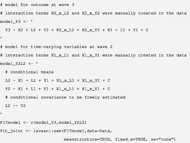
Box 3 Sample analysis code to estimate the parametric g-formula.

Here, we provide sample analysis code for fitting the models in Equations (16) and (17) in steps A1 and A2. The sample code uses an SEM approach with the lavaan package (Rosseel, 2012) in R (R Core Team, 2021). For illustration, we included only a single baseline covariate (C) and two covariate-treatment interactions. In practice, researchers may consider including a richer set of meaningful nonlinear and interaction terms when appropriate.

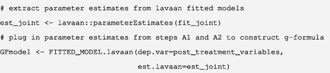
The parameter estimates can then be plugged in to construct an estimator of the parametric g-formula in Equation (11)(11) $$\begin{array}{l}{\mathrm{E}}_{(X_1,X_2)\leftarrow (1,0)}(Y_3)\\ =\sum _{c,l_1,y_1,l_2,y_2}\mathrm{E}(Y_3|x_2=0,l_2,y_2,x_1=1,l_1,y_1,c)\mathrm{p}(l_2,y_2|x_1=1,l_1,y_1,c)\mathrm{p}(c,l_1,y_1).\end{array}$$(11) . To help researchers implement this in practice, we have developed an R function FITTED_MODEL.lavaan requiring only two arguments: the post-treatment variables’ names and the parameter estimates from the fitted lavaan model.

In Appendix B, we apply the code above to the running example, present examples of the resulting model estimates using the observed data, and describe the inputs to the FITTED_MODEL.lavaan function.

Remarks

We make three remarks about estimating the parametric g-formula as described above. First, we need only specify regression models for the post-treatment variables that may be affected by at least one treatment instance, such as Y₃ in Equation (16)(16) $$\begin{array}{l}\mathrm{E}(Y_3|x_2,l_2,y_2,x_1,l_1,y_1,c)\\ ={\beta }_{y3,0}+{\beta }_{y3,x2}{x}_2+{\beta }_{y3,l2}{l}_2+{\beta }_{y3,y2}{y}_2+{\beta }_{y3,x2:l2}{x}_2{l}_2+{\beta }_{y3,x2:y2}{x}_2{y}_2+{\beta }_{y3,x1}{x}_1+{\beta }_{y3,l1}{l}_1+{\beta }_{y3,y1}{y}_1+{\beta }_{y3,c}c.\end{array}$$(16) , and L₂ and Y₂ in Equation (17)(17) $$\begin{array}{l}\left[\begin{array}{c}{L}_2\\ Y_2\end{array}\right]\sim {\mathcal{N}}_2\left(\left[\begin{array}{c}{\mu }_{L_2|x_1,l_1,y_1,c}\\ {\mu }_{Y_2|x_1,l_1,y_1,c}\end{array}\right],{\Sigma }_{L_2,Y_2|x_1,l_1,y_1,c}\right);\\ {\mu }_{L_2|x_1,l_1,y_1,c}={\beta }_{l2,0}+{\beta }_{l2,x1}{x}_1+{\beta }_{l2,l1}{l}_1+{\beta }_{l2,y1}{y}_1+{\beta }_{l2,x1:l1}{x}_1{l}_1+{\beta }_{l2,x1:y1}{x}_1{y}_1+{\beta }_{l2,c}c,\\ {\mu }_{Y_2|x_1,l_1,y_1,c}={\beta }_{y2,0}+{\beta }_{y2,x1}{x}_1+{\beta }_{y2,l1}{l}_1+{\beta }_{y2,y1}{y}_1+{\beta }_{y2,x1:l1}{x}_1{l}_1+{\beta }_{y2,x1:y1}{x}_1{y}_1+{\beta }_{y2,c}c,\\ {\Sigma }_{L_2,Y_2|x_1,l_1,y_1,c}=\left[\begin{array}{cc}{\sigma }_{l2}^2& {\sigma }_{l2,y2}\\ {\sigma }_{l2,y2}& {\sigma }_{y2}^2\end{array}\right].\end{array}$$(17) . This is because the stochastic components in the g-formula entail only the (time-varying) covariates and outcomes. Propensity score models (Rosenbaum & Rubin, 1983) for the treatments are not used because the treatments are uniformly fixed at specific levels (i.e., degenerate probability functions) in the g-formula. Second, there is no need to specify a model for the joint distribution of variables preceding the first treatment, i.e., $\mathrm{p}(c,l_1,y_1).$ This is because it can be estimated nonparametrically using its empirical distribution. We demonstrate this in the next section.

Third, in step A2, as stated in Robins et al. (1999, p. 698), at each timepoint t, only the joint distribution of concurrent time-varying covariates (such as L₂ and Y₂ at t = 2), conditional on all their causally preceding variables is necessary. As an alternative to utilizing their joint distribution, we can further factorize the joint probability, such as $\mathrm{p}(l_2,y_2|x_1,l_1,y_1,c),$ into a product of iterative conditional probabilities according to an arbitrary (noncausal) ordering, such as $\mathrm{p}(l_2|y_2,x_1,l_1,y_1,c)\mathrm{p}(y_2|x_1,l_1,y_1,c)$ or $\mathrm{p}(l_2|x_1,l_1,y_1,c)\mathrm{p}(y_2|l_2,x_1,l_1,y_1,c).$ Daniel et al. (2011), McGrath et al. (2020) and Taubman et al. (2009) offer detailed examples of developing such factorizations in the parametric g-formula. However, this can quickly become complicated when multiple concurrently measured time-varying variables exist in each timepoint. A specific complication that can sometimes arise is specifying different parametric models—possibly conditional on other time-varying variables within the same timepoint—that are compatible (or “congenial”; Meng, 1994) with one another. In contrast, an assumed model for their joint distribution, such as Equation (17)(17) $$\begin{array}{l}\left[\begin{array}{c}{L}_2\\ Y_2\end{array}\right]\sim {\mathcal{N}}_2\left(\left[\begin{array}{c}{\mu }_{L_2|x_1,l_1,y_1,c}\\ {\mu }_{Y_2|x_1,l_1,y_1,c}\end{array}\right],{\Sigma }_{L_2,Y_2|x_1,l_1,y_1,c}\right);\\ {\mu }_{L_2|x_1,l_1,y_1,c}={\beta }_{l2,0}+{\beta }_{l2,x1}{x}_1+{\beta }_{l2,l1}{l}_1+{\beta }_{l2,y1}{y}_1+{\beta }_{l2,x1:l1}{x}_1{l}_1+{\beta }_{l2,x1:y1}{x}_1{y}_1+{\beta }_{l2,c}c,\\ {\mu }_{Y_2|x_1,l_1,y_1,c}={\beta }_{y2,0}+{\beta }_{y2,x1}{x}_1+{\beta }_{y2,l1}{l}_1+{\beta }_{y2,y1}{y}_1+{\beta }_{y2,x1:l1}{x}_1{l}_1+{\beta }_{y2,x1:y1}{x}_1{y}_1+{\beta }_{y2,c}c,\\ {\Sigma }_{L_2,Y_2|x_1,l_1,y_1,c}=\left[\begin{array}{cc}{\sigma }_{l2}^2& {\sigma }_{l2,y2}\\ {\sigma }_{l2,y2}& {\sigma }_{y2}^2\end{array}\right].\end{array}$$(17) , will often be simpler to specify using SEM, an approach familiar to psychologists and established in the field.

Estimating the parameters in an MSM

With the estimators of the parametric g-formula in hand, we now turn to estimating the MSM in Equation (15)(15) $${\mathrm{E}}_{(X_1,X_2)\leftarrow (x_1,x_2)}(Y_3)={\psi }_0+{\psi }_1{x}_1+{\psi }_2{x}_2.$$(15) . We will use the regression models estimated in steps A1 and A2 to simulate the longitudinal counterfactual data forward in time. The procedure is as follows. We use the prefix “B” to designate each step of the MSM procedure.

B1. Construct an expanded data set for each individual containing all possible combinations of the treatment levels. Hence, each row corresponds to a different treatment sequence under the hypothetical manipulation of fixed levels $(X_1,X_2)\leftarrow (x_1,x_2),$ mutually exclusive from the other rows. For a binary treatment where $x_1,x_2\in \{0,1\},$ there would therefore be 2 × 2 = 4 rows. Across all rows, retain the same observed values of the pretreatment variables ($C,L_1,Y_1$) causally preceding the first treatment, but set the post-treatment variables ($L_2,Y_2,Y_3$) as missing. An example of the expanded data set for a single individual is shown in Table 2.

Table 2. Expanded data for a single individual used to estimate an MSM parametrizing the time-varying effects of treatment at two timepoints.

Step B1					Step B2		Step B3
C	L1	Y1	x1	x2	${\tilde{L}}_2(x_1)$	${\tilde{Y}}_2(x_1)$	$Y_3(x_1,x_2)$
C	L1	Y1	0	0	${\tilde{L}}_2(x_1=0)$	${\tilde{Y}}_2(x_1=0)$	$\widehat{h}(x_2=0,l_2={\tilde{L}}_2(0),y_2={\tilde{Y}}_2(0),x_1=0,L_1,Y_1,C)$
C	L1	Y1	0	1	${\tilde{L}}_2(x_1=0)$	${\tilde{Y}}_2(x_1=0)$	$\widehat{h}(x_2=1,l_2={\tilde{L}}_2(0),y_2={\tilde{Y}}_2(0),x_1=0,L_1,Y_1,C)$
C	L1	Y1	1	0	${\tilde{L}}_2(x_1=1)$	${\tilde{Y}}_2(x_1=1)$	$\widehat{h}(x_2=0,l_2={\tilde{L}}_2(1),y_2={\tilde{Y}}_2(1),x_1=0,L_1,Y_1,C)$
C	L1	Y1	1	1	${\tilde{L}}_2(x_1=1)$	${\tilde{Y}}_2(x_1=1)$	$\widehat{h}(x_2=1,l_2={\tilde{L}}_2(1),y_2={\tilde{Y}}_2(1),x_1=0,L_1,Y_1,C)$

Notes. There are four rows corresponding to all possible combinations of a binary treatment occurring at two timepoints. For each row, the contents are filled in column-wise from left to right, possibly conditional on values in the columns to the left, with each step indicated in the heading and described in the main text. For example, in step B2, the counterfactual covariate and outcome, ${\tilde{L}}_2(x_1)$ and ${\tilde{Y}}_2(x_1),$ respectively, denote Monte Carlo random draws from their counterfactual joint distribution conditional on the observed pretreatment variables ($C,L_1,Y_1$) and fixed treatment level X₁ = x₁. The imputed potential outcome under hypothetical treatment levels x₁ and x₂ are denoted by $Y_3(x_1,x_2),$ and are used to calculate the average potential outcome ${\mathrm{E}}_{(X_1,X_2)\leftarrow (x_1,x_2)}(Y_3)$ in the MSM.

B2. For each row with a given treatment sequence (x₁, x₂) in turn, randomly sample a value of the counterfactual time-varying variables ${\tilde{L}}_2(x_1)$ and ${\tilde{Y}}_2(x_1)$ from their estimated joint distribution ${\widehat{F}}_{L_2,Y_2}(l_2,y_2|x_1,l_1=L_1,y_1=Y_1,c=C)$ from Equation (17)(17) $$\begin{array}{l}\left[\begin{array}{c}{L}_2\\ Y_2\end{array}\right]\sim {\mathcal{N}}_2\left(\left[\begin{array}{c}{\mu }_{L_2|x_1,l_1,y_1,c}\\ {\mu }_{Y_2|x_1,l_1,y_1,c}\end{array}\right],{\Sigma }_{L_2,Y_2|x_1,l_1,y_1,c}\right);\\ {\mu }_{L_2|x_1,l_1,y_1,c}={\beta }_{l2,0}+{\beta }_{l2,x1}{x}_1+{\beta }_{l2,l1}{l}_1+{\beta }_{l2,y1}{y}_1+{\beta }_{l2,x1:l1}{x}_1{l}_1+{\beta }_{l2,x1:y1}{x}_1{y}_1+{\beta }_{l2,c}c,\\ {\mu }_{Y_2|x_1,l_1,y_1,c}={\beta }_{y2,0}+{\beta }_{y2,x1}{x}_1+{\beta }_{y2,l1}{l}_1+{\beta }_{y2,y1}{y}_1+{\beta }_{y2,x1:l1}{x}_1{l}_1+{\beta }_{y2,x1:y1}{x}_1{y}_1+{\beta }_{y2,c}c,\\ {\Sigma }_{L_2,Y_2|x_1,l_1,y_1,c}=\left[\begin{array}{cc}{\sigma }_{l2}^2& {\sigma }_{l2,y2}\\ {\sigma }_{l2,y2}& {\sigma }_{y2}^2\end{array}\right].\end{array}$$(17) . For the values of the predictors, set the first treatment at timepoint 1 to the hypothetical fixed level X₁ = x₁, and retain the observed values of the remaining pretreatment variables ($C,L_1,Y_1$). More generally, the counterfactual variables at time t are simulated based on the fixed treatment levels only through time t – 1. We use a tilde (∼) overhead symbol to emphasize these are stochastically drawn counterfactual values.

B3. For each row with a given treatment sequence (x₁, x₂) in turn, impute the potential outcome, denoted by $Y_3(x_1,x_2),$ as a prediction from the fitted outcome model $h(x_2,l_2={\tilde{L}}_2(x_1),y_2={\tilde{Y}}_2(x_1),x_1,l_1=L_1,y_1=Y_1,c=C)$ from Equation (16)(16) $$\begin{array}{l}\mathrm{E}(Y_3|x_2,l_2,y_2,x_1,l_1,y_1,c)\\ ={\beta }_{y3,0}+{\beta }_{y3,x2}{x}_2+{\beta }_{y3,l2}{l}_2+{\beta }_{y3,y2}{y}_2+{\beta }_{y3,x2:l2}{x}_2{l}_2+{\beta }_{y3,x2:y2}{x}_2{y}_2+{\beta }_{y3,x1}{x}_1+{\beta }_{y3,l1}{l}_1+{\beta }_{y3,y1}{y}_1+{\beta }_{y3,c}c.\end{array}$$(16) . The prediction is based on: (i) fixed treatment levels X₁ = x₁ and X₂ = x₂, (ii) randomly drawn values of the counterfactual time-varying variables ${\tilde{L}}_2(x_1)$ and ${\tilde{Y}}_2(x_1)$ from the previous step, and (iii) observed values of the covariate L₁, outcome Y₁, and baseline covariates C preceding the first treatment.

B4. Repeat steps B1 to B3 100 times to generate 100 pseudo-copies of the expanded data sets. (As discussed below, more pseudo-copies will produce more precise results.) For each individual, the observed values of the variables preceding the first treatment ($C,L_1,Y_1$) are the same; only the random draws of the counterfactual time-varying variables ${\tilde{L}}_2(x_1)$ and ${\tilde{Y}}_2(x_1),$ and predicted potential outcome $Y_3(x_1,x_2),$ may differ across pseudo-copies. Then, concatenate all 100 pseudo-copies to yield a single enlarged data set (with $100\times 4\times N$ rows).

B5. Fit the MSM in Equation (15)(15) $${\mathrm{E}}_{(X_1,X_2)\leftarrow (x_1,x_2)}(Y_3)={\psi }_0+{\psi }_1{x}_1+{\psi }_2{x}_2.$$(15) to the single enlarged data set using ordinary least squares. In doing so, we average over the (counterfactual) distribution of the time-varying variables (L₂, Y₂), and the empirical distribution of the variables preceding the first treatment ($C,L_1,Y_1$), using Monte Carlo integration.

Box 4 Sample analysis code to estimate an MSM using the parametric g-formula.

How do we estimate an MSM using the parametric g-formula? To help researchers implement the procedure, we have developed a single R function (“FitMSM”) that carries out all the above steps B1 to B5.

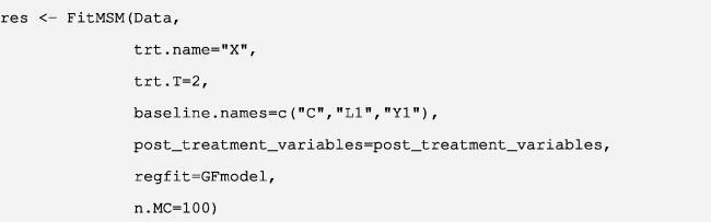
In Appendix C, we describe the inputs to the function and apply it to the observed data from our running example.

Remarks

Nonparametric percentile bootstrap confidence intervals (Efron & Tibshirani, 1994) may be constructed by randomly resampling observations with replacement and repeating all the above steps (A1 and A2, and B1 to B5) for each bootstrap sample. We emphasize that the model-based standard errors and confidence intervals from fitting the MSM to the single enlarged data set in step B5 cannot be used for statistical inference because they do not accurately reflect the sampling variability and will lead to biased statistical inferences.

Finally, we briefly discuss step B4, generating the pseudo-copies. We emphasize that the same observed values of the variables preceding the first treatment ($C,L_1,Y_1$) are retained across pseudo-copies. Therefore, averaging over these pseudo-copies provides a Monte Carlo approximation of the average over their empirical distribution $\mathrm{p}(c,l_1,y_1);$ see Robert and Casella (2010, Chapter 3) for a general introduction to Monte Carlo integration. For our illustration, we used 100 pseudo-copies as an example of Monte Carlo integration. In practice, researchers should strive to use as many pseudo-copies as computationally feasible to minimize Monte Carlo simulation error and increase precision. Hence, increasing the number of pseudo-copies incurs the cost of increasing computation time, especially with the use of the nonparametric bootstrap for statistical inference. If computation time becomes unacceptably long, an alternative to utilizing multiple pseudo-copies of every individual is to use a random subset of the original data set to construct a single enlarged data set, as carried out in existing implementations of the parametric g-formula (Daniel et al., 2011; McGrath et al., 2020).

Box 5 Interpreting the results from the parametric g-formula.

The estimated effect of loneliness at timepoint 1 on friendship quality was ${\psi }_1=-0.22;$ $95\%\text{CI}=(-0.36,-0.07),$ and the estimated effect of loneliness at timepoint 2 was ${\psi }_2=-0.18;$ $95\%\text{CI}=(-0.32,-0.04).$ Confidence intervals (CIs) were calculated using 1000 nonparametric bootstrap samples with replacement. These results showed that loneliness undermined friendship quality over time. Specifically, earlier loneliness (at timepoint 1) reduced friendship quality (at timepoint 3) by 0.22 on a five-point scale, while more recent loneliness (at timepoint 2) reduced friendship quality (at timepoint 3) by 0.18 on a five-point scale. These results provide support to the theoretical perspective that loneliness is not only a consequence but also a cause of poor social relationships (Stavrova & Ren, 2023). These results also highlight the importance of examining the causal effects of longer lags because a treatment’s impact can take time to unfold. The steps to implement the parametric g-formula are summarized in Figure 2.

Discussion

The g-formula is an elegant and effective method for testing time-varying treatment effects in the presence of measured treatment-dependent confounding. In this paper, we presented the parametric g-formula using standard multiple linear regression functions, which are familiar to psychological researchers. We leveraged this crucial correspondence to describe how to implement the parametric g-formula using lavaan, a popular structural equation modeling package.

In doing so, we utilized various features implemented in lavaan to calculate quantities needed in the parametric g-formula. The joint counterfactual distribution of multiple concurrent time-varying confounders within each timepoint, conditional on all causally preceding variables, can be parsimoniously modeled using lavaan. A benefit of using lavaan is the ease with which parameter constraints can be introduced in the lavaan model syntax. For example, the lag 1 effects of X_t on $Y_{t+1}$ can be readily constrained to be constant over time; similarly, the autoregressive effects of Y_t on $Y_{t+1}$ can also be constrained to be stable over time. Another advantage of utilizing lavaan is the ability to employ missing data methods to account for intermittently missing data—often encountered when using longitudinal designs in practice—after establishing that missingness is at random (MAR; Leyrat et al., 2021; Potthoff et al., 2006). “Full information” maximum likelihood estimation (Enders, 2022; Lee & Shi, 2021) can be readily incorporated when fitting the models to the original observed data in steps A1 and A2 (e.g., by including the argument missing = “ML” when using lavaan).

Limitations and related work

Like all approaches to causal inference, the validity of effects estimated using the g-formula rests on meeting the assumptions of the approach. The key assumption of the g-formula is sequential ignorability: the available covariates must suffice for confounding adjustment. Within the causal diagram in Figure 1, the sequential ignorability assumption is represented by the (i) omission of arrows between either U or U_t and treatment (X₁ or X₂); and (ii) absence of hidden common causes of treatment (X₁ or X₂), and the outcomes (Y₁, Y₂, or Y₃). Therefore, researchers should strive to measure a rich set of putative time-invariant and time-varying covariates (Daniel et al., 2013). Steiner et al. (2010) provide practical recommendations for selecting confounders. In addition to the sequential ignorability assumption, two other assumptions common to all causal inferential methods must be met. The first is positivity (Petersen et al., 2012), whereby each individual must have nonzero probabilities of being assigned to each possible treatment level, given their pretreatment covariates. This ensures that $\mathrm{p}(x_2,l_2,y_2,x_1,l_1,y_1,c)>0$ for all values of the variables, thus avoiding conditioning on events with zero probability of occurring and yielding ill-defined effects in nonexistent covariate strata (Rudolph et al., 2022). The second is causal, or counterfactual, consistency (Pearl, 2010), which states that when a hypothetical treatment sequence equals the observed treatment levels, the potential outcomes and the actually observed outcomes must be identical.

There are also other scenarios where sequential ignorability may be violated, such as when unobserved stable traits (e.g., U in Figure 1) affect both treatment and outcome. To address this, a different approach in psychological research is to statistically control for such latent traits; see, e.g., Andersen (2022); Usami et al. (2019) for discussions of methods under this approach in a different context. These statistical models incorporate stable traits as latent variables or random intercepts and focus on within-person effects adjusted for these traits when analyzing longitudinal panel data. Lüdtke and Robitzsch (2022) compare and contrast these different approaches when focusing on lag-1 causal effects. We recommend researchers measure both time-invariant baseline characteristics and time-varying covariates toward bolstering the sequential ignorability assumption (VanderWeele et al., 2016, 2020) when aiming for valid causal inferences of time-varying treatment effects using the parametric g-formula.

For ease of exposition, we have limited our presentation to a marginal structural model (MSM) with only main effects whose parameters represent average causal effects for the entire study or source population (Robins et al., 2000). However, an MSM with covariate-treatment interactions can also be posited to test effect heterogeneity due to putative baseline time-invariant covariates (Breskin et al., 2018; VanderWeele, 2009). For MSMs involving interactions between a binary treatment and continuous covariates, we recommend that the treatments be effect-coded and the covariates mean-centered to facilitate meaningful interpretations of the causal effects parameterized in the MSM (West et al., 1996). Extensions of MSMs to investigate effect heterogeneity are deferred to future work.

The imputation-based estimation procedure we presented follows the procedures proposed by Snowden et al. (2011), Taubman et al. (2009), Westreich et al. (2012), and shares their strengths and challenges (Vansteelandt & Keiding, 2011). In particular, consistent estimation of the causal parameters in the MSM (15) relies on correctly specifying both regression models (16) and (17). To reduce the risks of biases due to incorrectly specifying regression models (16) and (17), saturated or richly parameterized models with various prespecified interactions and higher-order terms, or flexible nonlinear functional forms (e.g., splines; Suk et al., 2019), for the predictors can be fitted instead. However, in practice, it may be difficult or even impossible to fit such models due to the curse of dimensionality. Alternatively, in Appendix D, we propose a heuristic doubly robust variant that can help protect against biases from incorrectly specified mean models for the post-treatment variables using a correctly specified propensity score model.

The parameters of an MSM can be consistently estimated using the g-formula, as presented in this paper. An alternative approach is to use inverse probability of treatment weighting (IPW) (Robins et al., 2000). IPW utilizes only a series of propensity score models for the treatment at each timepoint, conditional on the measured pretreatment covariate history; see, e.g., Kennedy et al. (2022), Thoemmes and Ong (2015), and Vandecandelaere et al. (2016) for applications in the psychological literature. In contrast, the parametric g-formula models the (counterfactual) distributions of all post-treatment variables, such as L₂, Y₂, and Y₃, that are conditional on the preceding treatments and measured pretreatment covariate history. The parametric g-formula has two advantages over IPW. First, the parametric g-formula utilizes regression models for the time-varying variables which are already familiar to psychologists. Second, under correctly specified parametric models, parametric g-formula estimates may have smaller standard errors and smaller finite sample biases than IPW estimates; see, e.g., Daniel et al. (2013) for a comparison of these two methods. Finally, although the names may be confusingly similar, we emphasize that the g-formula is different from another established g-method called g-estimation (Robins, 1997). G-estimation is used to estimate the causal parameters encoded in a structural nested mean model describing the potential outcomes’ functional dependence on treatments. G-estimation has only recently been introduced to the psychology literature (Loh, 2024; Loh & Ren, 2023b); see Loh and Ren (2023a) for a nontechnical introduction with an implementation using lavaan.

For ease of presentation, we limited our development to continuous post-treatment variables, such as L₂ and Y₃, so that linear regression functions for these variables could be reasonably assumed. It is important to note that the parametric g-formula applies to continuous and noncontinuous time-varying variables, with any plausible (parametric) model for their conditional distribution or mean. For example, if L_t is an ordered categorical variable, an ordinal logistic regression model for its conditional distribution may be assumed. Or if Y_t is a time-to-event outcome subject to right-censoring (where the events may not occur during the duration of the study), survival models for the discretized time-varying event indicator may be specified (Keil et al., 2014; McGrath et al., 2020; Westreich et al., 2012).

In this paper, we considered only so-called “static” treatment sequences, in which the treatment at each timepoint was deterministically fixed to a prespecified value. In our running example, a static treatment sequence $(X_1=1,X_2=0$) corresponds to hypothetically manipulating all participants to feel lonely at timepoint 1 ($X_1=1$) but to feel not lonely at timepoint 2 ($X_2=0$). Developments in adaptive trial designs have utilized so-called “dynamic” treatment regimes that assign treatment at each timepoint depending on historical values of preceding variables (Petersen et al., 2014; Robins, 1986; Young et al., 2011; Zhang et al., 2018). This history may include observed or counterfactual values of the time-varying variables. Continuing our running example, researchers may be interested in understanding the average friendship quality at timepoint 3 under a dynamic treatment regime where students “do not feel lonely in timepoint 1 ($X_1=0$) but feel lonely later in timepoint 2 ($X_2=1$) only if intermediate friendship quality falls below a fixed threshold d ($Y_2(x_1=0)<d$).” Studies enforcing strict rules on participants’ treatments can be conceptually and practically challenging. The parametric g-formula permits estimation of the effects of such dynamic treatment regimes using properly analyzed observational studies (Young et al., 2011; Zhang et al., 2018).

Conclusion

In longitudinal studies where treatments vary over time, treatment-dependent or time-varying confounding presents a pernicious challenge to valid causal inferences. The parametric g-computation formula, or simply g-formula, provides an established and practical solution for effectively handling measured treatment-dependent confounding. In this article, we described how to implement the parametric g-formula using familiar parametric regression functions. We utilized the accessible and popular lavaan package in R to implement the parametric g-formula. Moreover, we described how to use the estimators from the parametric g-formula to fit a marginal structural model that delivers parsimonious inferences about the causal effects of a time-varying treatment. The parametric g-formula is effective, intuitive, and easy to implement. We encourage psychological researchers pursuing causal inferences in longitudinal studies to employ the parametric g-formula when testing the causal effects of a time-varying treatment.

Article information

Conflict of interest disclosures: Each author signed a form for disclosure of potential conflicts of interest. No authors reported any financial or other conflicts of interest in relation to the work described.

Ethical principles: The authors affirm having followed professional ethical guidelines in preparing this work. These guidelines include obtaining informed consent from human participants, maintaining ethical treatment and respect for the rights of human or animal participants, and ensuring the privacy of participants and their data, such as ensuring that individual participants cannot be identified in reported results or from publicly available original or archival data.

Funding: Wen Wei Loh was partially supported by the University Research Committee (URC) Regular Award of Emory University, Atlanta, Georgia, USA.

Role of the funders/sponsors: None of the funders or sponsors of this research had any role in the design and conduct of the study; collection, management, analysis, and interpretation of data; preparation, review, or approval of the manuscript; or decision to submit the manuscript for publication.

Acknowledgments: The authors thank the Editor in Chief, Dr. Alberto Maydeu-Olivares, for his invaluable advice in guiding the manuscript through the review process. The authors thank all three anonymous reviewers for their insightful and helpful comments, which have greatly improved the manuscript. The authors thank Dr. Louise Poppe of Ghent University for feedback on an earlier draft. The ideas and opinions expressed herein are those of the authors alone, and endorsement by the authors’ institutions is not intended and should not be inferred.

Open Scholarship

This article has earned the Center for Open Science badges for Open Data and Open Materials through Open Practices Disclosure. The data and materials are openly accessible at https://doi.org/10.3886/ICPSR34598.v1 and https://github.com/wwloh/gformula-lavaan.

Additional information

Funding

Wen Wei Loh was partially supported by the University Research Committee (URC) Regular Award of Emory University, Atlanta, Georgia, USA.

Notes

1 Other structural equation modeling software, such as Amos (Arbuckle, 2019), PROC CALIS (Hatcher, 1996), Mplus (Muthén & Muthén, 1998–2017), and OpenMx (Boker et al., 2011), can also be used, but lavaan offers seamless integration with the R functions we provide to implement the parametric g-formula.

2 In this paper, we assume that researchers can justifiably postulate a causal diagram based on established knowledge and temporal-logical constraints. Readers are referred to Digitale et al. (2022), Elwert (2013), Grosz et al. (2020), and Rohrer (2018), among others, for accessible introductions to the causal diagram framework.

3 The unmeasured variables U and U_t allow for residual correlations among the outcome errors, e.g., due to hidden common causes or latent processes, when the outcome is repeatedly measured; see, e.g., Loh and Ren (2023c) for a probative example with two time points. When it can be theoretically justified that U and U_t are completely observed so that any unmeasured confounding of the repeatedly measured outcomes can be ruled out, the problems induced by treatment-dependent confounding disappear, and standard regression methods can yield valid inferences (Daniel et al., 2013; Moodie & Stephens, 2010; Robins et al., 2000). In this case, the g-formula approach is unnecessary.

4 Following Daniel et al. (2011, p. 486), we use $\mathrm{p}(a|b)$ interchangeably in referring to either (i) the probability density function if A is continuous or (ii) the probability mass function if A is discrete. Following McGrath et al. (2020, Supplemental Online Materials Section A.3), we use for notational simplicity a summation symbol when calculating an expectation; when there are continuous random variables (such as L and Y in this paper), the sums may be replaced with integrals. This convention of using the summation notation when expressing the parametric g-formula has previously been adopted in the causal inference literature (see selected examples listed in the introduction). We acknowledge that the validity of the parametric g-formula when there are continuous variables is subject to certain continuity assumptions being met to permit the use of conditional probability density functions (Gill & Robins, 2001). Readers interested in the theoretical mathematical details of generalizing the g-formula from the discrete-only setting to the continuous case are referred to Gill and Robins (2001).

5 These deterministic indicator functions represent (degenerate) probability functions that place probability one on the atomic or elementary events $X_1=1$ and $X_2=0$ (and probability zero on all other values of X₁ and X₂).

6 Mean-centering the continuous variables at each time point (e.g., L₂ and Y₂) facilitates meaningful interpretations of first-order effects used in models containing categorical by continuous variable interactions (West et al., 1996). However, we emphasize that these model coefficients do not encode the causal effects parameterized in the MSM, and inferences and interpretations of the treatment effects should not be based on this model alone.

7 The parametric label arises from the use of parametric non-saturated (regression) models for the conditional mean or distribution of the post-treatment variables, such as Equations (16)(16) $$\begin{array}{l}\mathrm{E}(Y_3|x_2,l_2,y_2,x_1,l_1,y_1,c)\\ ={\beta }_{y3,0}+{\beta }_{y3,x2}{x}_2+{\beta }_{y3,l2}{l}_2+{\beta }_{y3,y2}{y}_2+{\beta }_{y3,x2:l2}{x}_2{l}_2+{\beta }_{y3,x2:y2}{x}_2{y}_2+{\beta }_{y3,x1}{x}_1+{\beta }_{y3,l1}{l}_1+{\beta }_{y3,y1}{y}_1+{\beta }_{y3,c}c.\end{array}$$(16) and (17)(17) $$\begin{array}{l}\left[\begin{array}{c}{L}_2\\ Y_2\end{array}\right]\sim {\mathcal{N}}_2\left(\left[\begin{array}{c}{\mu }_{L_2|x_1,l_1,y_1,c}\\ {\mu }_{Y_2|x_1,l_1,y_1,c}\end{array}\right],{\Sigma }_{L_2,Y_2|x_1,l_1,y_1,c}\right);\\ {\mu }_{L_2|x_1,l_1,y_1,c}={\beta }_{l2,0}+{\beta }_{l2,x1}{x}_1+{\beta }_{l2,l1}{l}_1+{\beta }_{l2,y1}{y}_1+{\beta }_{l2,x1:l1}{x}_1{l}_1+{\beta }_{l2,x1:y1}{x}_1{y}_1+{\beta }_{l2,c}c,\\ {\mu }_{Y_2|x_1,l_1,y_1,c}={\beta }_{y2,0}+{\beta }_{y2,x1}{x}_1+{\beta }_{y2,l1}{l}_1+{\beta }_{y2,y1}{y}_1+{\beta }_{y2,x1:l1}{x}_1{l}_1+{\beta }_{y2,x1:y1}{x}_1{y}_1+{\beta }_{y2,c}c,\\ {\Sigma }_{L_2,Y_2|x_1,l_1,y_1,c}=\left[\begin{array}{cc}{\sigma }_{l2}^2& {\sigma }_{l2,y2}\\ {\sigma }_{l2,y2}& {\sigma }_{y2}^2\end{array}\right].\end{array}$$(17) , when there are multiple continuous predictors in each model. In contrast, a non-parametric g-formula is feasible only in simple settings where the predictors are discrete so that a saturated model for each conditional mean or probability function can be fitted (thereby avoiding parametric modeling assumptions) while ensuring that the positivity assumption is met; see, e.g., Daniel et al. (2013) and Naimi et al. (2016).

8 A correctly specified propensity score model can offer protection from biases due to certain forms of misspecification in the regression model(s) when estimating the treatment effects. However, the parametric g-formula relies on correctly specifying models for the distribution, not just the mean, of all post-treatment covariates (other than the final outcome). It may be possible that the full distribution remains vulnerable to certain model misspecification biases, even after weighting by the inverse probabilities of treatment; e.g., when distributional assumptions (such as normality and constant variance) in Equation (17)(17) $$\begin{array}{l}\left[\begin{array}{c}{L}_2\\ Y_2\end{array}\right]\sim {\mathcal{N}}_2\left(\left[\begin{array}{c}{\mu }_{L_2|x_1,l_1,y_1,c}\\ {\mu }_{Y_2|x_1,l_1,y_1,c}\end{array}\right],{\Sigma }_{L_2,Y_2|x_1,l_1,y_1,c}\right);\\ {\mu }_{L_2|x_1,l_1,y_1,c}={\beta }_{l2,0}+{\beta }_{l2,x1}{x}_1+{\beta }_{l2,l1}{l}_1+{\beta }_{l2,y1}{y}_1+{\beta }_{l2,x1:l1}{x}_1{l}_1+{\beta }_{l2,x1:y1}{x}_1{y}_1+{\beta }_{l2,c}c,\\ {\mu }_{Y_2|x_1,l_1,y_1,c}={\beta }_{y2,0}+{\beta }_{y2,x1}{x}_1+{\beta }_{y2,l1}{l}_1+{\beta }_{y2,y1}{y}_1+{\beta }_{y2,x1:l1}{x}_1{l}_1+{\beta }_{y2,x1:y1}{x}_1{y}_1+{\beta }_{y2,c}c,\\ {\Sigma }_{L_2,Y_2|x_1,l_1,y_1,c}=\left[\begin{array}{cc}{\sigma }_{l2}^2& {\sigma }_{l2,y2}\\ {\sigma }_{l2,y2}& {\sigma }_{y2}^2\end{array}\right].\end{array}$$(17) are violated. Closer examination and more formal theoretical demonstrations of the double robustness property are deferred to future work.

9 In principle, under the linear and additive regression models assumed here, one could use standard product-of-coefficient estimators for the combined path-specific effects that make up each causal effect. But this is realistic only with regression models having only main effects. When interactions or higher-order terms are specified, as in the running example, deriving closed-form expressions of the effect estimators can be complicated in practice. Furthermore, the number of possible paths grows exponentially with the number of time points and time-varying covariates. In general, for k treatment-dependent confounders at T time points between treatment and outcome, there are ${(k+1)}^T$ possible paths; e.g., if k = 2 and T = 3, there are 27 different paths. We, therefore, do not recommend such an approach.

10 We used a sample size of 1000 merely to illustrate that the biases due to: (i) inappropriate adjustment for time-varying confounding using a routine regression method; and (ii) an incorrectly-specified outcome regression function using the parametric g-formula without the doubly-robust variant, persist with a relatively large sample size. Because using smaller sample sizes introduces finite sample variability across all the estimators, thus complicating disentangling the systematic and finite sample biases, we defer more comprehensive examinations of the various estimators’ operating characteristics under different sample sizes to future work.

11 It could be argued that the coefficient of X₁ in the outcome model for Y is not a consistent estimator of the total effect because the regression coefficient encodes only the direct effect of X₁ on Y that is not transmitted via the intervening time-varying covariate L₂; see, e.g., Schisterman et al. (2009). But the estimator of the coefficient of X₁ will be biased due to the collider L₂ along the path $X_1\to L_2\leftarrow U\to Y_3;$ see the main text for a more detailed explanation.

Appendices Appendix A.

Details of data used in the running example

We briefly describe the data from the Flint Adolescent Study (Zimmerman, 2014) used in our running example. We utilized three waves of the survey: $1995 (t=1),1996 (t=2),$ and $1997 (t=3).$ The treatment X_t (loneliness) was the binary (yes or no) response to whether the student felt uncomfortable from feeling lonely during the past week (including the day of the interview). About half the students felt lonely at t = 1, but only half of those students subsequently felt lonely at t = 2. For the remaining half who did not feel lonely at t = 1, about 58% subsequently felt lonely at t = 2. The time-varying covariate L_t (family school support) was measured using the mean score of seven items on how the students’ parent(s) would support them if their academic performance were to decline, such as helping with homework, talking to teachers, and getting a tutor. Responses were on a four-point Likert scale (1 = Not at all likely; 4 = Very likely). The outcome Y_t (friendship quality) was measured using the mean score for five items on how the student supported and relied on support from their friends, such as whether they rely on their friends for emotional support, whether their friends come to them for emotional support, and whether their friends give them the moral support they need. Responses were on a five-point Likert scale (1 = Not true; 5 = Very true). The baseline covariates C were the following self-reported variables: age cohort (1 if their birth year was 1980, 0 if earlier than 1980), gender (1 for female, 0 for male), race (1 for Black or African American, 0 otherwise), and family socioeconomic status (1 if their family received income support, 0 otherwise). We considered the 749 students with complete data on these variables. For expository purposes of simplifying our introduction of the parametric g-formula in this paper, we ignored the clustered data structure (students within classrooms within schools). In practice, classroom- and school-level heterogeneity should be adjusted for (e.g., by modeling classroom and school identifiers as fixed or random effects) to achieve valid statistical inferences; see Hong and Raudenbush (2006), Kim and Steiner (2020), and Thoemmes and West (2011) for discussions on handling clustered data for treatment at a single timepoint. A snapshot of the data for seven students is presented in Table A1.

Table A1. Observed data for seven students in the running example.

ID	Gender	Race	Age	Income	X1	X2	L1	L2	Y1	Y2	Y3
100	1	1	1	1	1	1	0.35	0.31	1.62	−0.55	−0.68
205	1	1	0	1	0	0	0.64	0.60	1.02	0.45	−0.48
307	1	1	1	1	1	1	−0.93	−0.12	0.62	1.05	0.32
408	1	0	1	1	0	1	−0.08	0.31	0.82	−0.35	1.12
512	0	1	1	1	0	0	0.21	0.74	1.62	1.25	1.72
617	1	1	1	1	0	0	−0.36	0.45	0.02	−0.15	0.12
719	1	1	1	1	0	1	−0.22	0.31	0.22	0.65	−0.28

Notes. “Income” = family socioeconomic status; $X_t=$ whether they felt lonely or not lonely at time t; $L_t=$ family support with school at time t; $Y_t=$ friendship quality (support given to and from friends) at time t. The continuous variables L_t and Y_t were mean-centered. The values for each variable are defined in the text of Appendix A.

Appendix B.

Example of steps A1 and A2 using lavaan for the running example

In this section, we will use lavaan (Rosseel, 2012) to illustrate how to carry out steps A1 and A2 of the estimation procedure, by applying it to the data from the running example. We define the labels of the variables in our dataset as:

• LONELY__1 = X₁

• LONELY__2 = X₂

• FAMILY__1 = L₁

• FAMILY__2 = L₂

• FRIEND__1 = Y₁

• FRIEND__2 = Y₂

• FRIEND__3 = Y₃

The treatment-covariate interactions, calculated as the products of the respective variables, are labeled as:

• LONELY__1_x_FAMILY__1 = $X_1\times L_1$

• LONELY__1_x_FRIEND__1 = $X_1\times Y_1$

• LONELY__2_x_FAMILY__2 = $X_2\times L_2$

• LONELY__2_x_FRIEND__2 = $X_2\times Y_2$

First, we specify the outcome regression model in Equation (16)(16) $$\begin{array}{l}\mathrm{E}(Y_3|x_2,l_2,y_2,x_1,l_1,y_1,c)\\ ={\beta }_{y3,0}+{\beta }_{y3,x2}{x}_2+{\beta }_{y3,l2}{l}_2+{\beta }_{y3,y2}{y}_2+{\beta }_{y3,x2:l2}{x}_2{l}_2+{\beta }_{y3,x2:y2}{x}_2{y}_2+{\beta }_{y3,x1}{x}_1+{\beta }_{y3,l1}{l}_1+{\beta }_{y3,y1}{y}_1+{\beta }_{y3,c}c.\end{array}$$(16) using lavaan model syntax as:

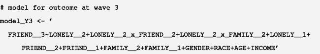
Next, we specify the model for the time-varying variables in Equation (17)(17) $$\begin{array}{l}\left[\begin{array}{c}{L}_2\\ Y_2\end{array}\right]\sim {\mathcal{N}}_2\left(\left[\begin{array}{c}{\mu }_{L_2|x_1,l_1,y_1,c}\\ {\mu }_{Y_2|x_1,l_1,y_1,c}\end{array}\right],{\Sigma }_{L_2,Y_2|x_1,l_1,y_1,c}\right);\\ {\mu }_{L_2|x_1,l_1,y_1,c}={\beta }_{l2,0}+{\beta }_{l2,x1}{x}_1+{\beta }_{l2,l1}{l}_1+{\beta }_{l2,y1}{y}_1+{\beta }_{l2,x1:l1}{x}_1{l}_1+{\beta }_{l2,x1:y1}{x}_1{y}_1+{\beta }_{l2,c}c,\\ {\mu }_{Y_2|x_1,l_1,y_1,c}={\beta }_{y2,0}+{\beta }_{y2,x1}{x}_1+{\beta }_{y2,l1}{l}_1+{\beta }_{y2,y1}{y}_1+{\beta }_{y2,x1:l1}{x}_1{l}_1+{\beta }_{y2,x1:y1}{x}_1{y}_1+{\beta }_{y2,c}c,\\ {\Sigma }_{L_2,Y_2|x_1,l_1,y_1,c}=\left[\begin{array}{cc}{\sigma }_{l2}^2& {\sigma }_{l2,y2}\\ {\sigma }_{l2,y2}& {\sigma }_{y2}^2\end{array}\right].\end{array}$$(17) as:

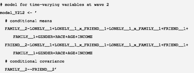
Both models (16) and (17) can be fitted simultaneously to the observed data using the sem function as follows:

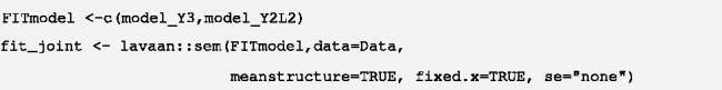
MLEs of the model parameters can then be extracted to estimate the parametric g-formula. The full set of parameter estimates are available online as part of the Supplemental Online Materials. As an example, the estimated error covariance between L₂ and Y₂ parametrized by ${\sigma }_{l2,y2}$ in Equation (17)(17) $$\begin{array}{l}\left[\begin{array}{c}{L}_2\\ Y_2\end{array}\right]\sim {\mathcal{N}}_2\left(\left[\begin{array}{c}{\mu }_{L_2|x_1,l_1,y_1,c}\\ {\mu }_{Y_2|x_1,l_1,y_1,c}\end{array}\right],{\Sigma }_{L_2,Y_2|x_1,l_1,y_1,c}\right);\\ {\mu }_{L_2|x_1,l_1,y_1,c}={\beta }_{l2,0}+{\beta }_{l2,x1}{x}_1+{\beta }_{l2,l1}{l}_1+{\beta }_{l2,y1}{y}_1+{\beta }_{l2,x1:l1}{x}_1{l}_1+{\beta }_{l2,x1:y1}{x}_1{y}_1+{\beta }_{l2,c}c,\\ {\mu }_{Y_2|x_1,l_1,y_1,c}={\beta }_{y2,0}+{\beta }_{y2,x1}{x}_1+{\beta }_{y2,l1}{l}_1+{\beta }_{y2,y1}{y}_1+{\beta }_{y2,x1:l1}{x}_1{l}_1+{\beta }_{y2,x1:y1}{x}_1{y}_1+{\beta }_{y2,c}c,\\ {\Sigma }_{L_2,Y_2|x_1,l_1,y_1,c}=\left[\begin{array}{cc}{\sigma }_{l2}^2& {\sigma }_{l2,y2}\\ {\sigma }_{l2,y2}& {\sigma }_{y2}^2\end{array}\right].\end{array}$$(17) is:

The estimated coefficient of X₁, ${\beta }_{y3,x1},$ in Equation (16)(16) $$\begin{array}{l}\mathrm{E}(Y_3|x_2,l_2,y_2,x_1,l_1,y_1,c)\\ ={\beta }_{y3,0}+{\beta }_{y3,x2}{x}_2+{\beta }_{y3,l2}{l}_2+{\beta }_{y3,y2}{y}_2+{\beta }_{y3,x2:l2}{x}_2{l}_2+{\beta }_{y3,x2:y2}{x}_2{y}_2+{\beta }_{y3,x1}{x}_1+{\beta }_{y3,l1}{l}_1+{\beta }_{y3,y1}{y}_1+{\beta }_{y3,c}c.\end{array}$$(16) is:

However, we emphasize that even when Equation (16)(16) $$\begin{array}{l}\mathrm{E}(Y_3|x_2,l_2,y_2,x_1,l_1,y_1,c)\\ ={\beta }_{y3,0}+{\beta }_{y3,x2}{x}_2+{\beta }_{y3,l2}{l}_2+{\beta }_{y3,y2}{y}_2+{\beta }_{y3,x2:l2}{x}_2{l}_2+{\beta }_{y3,x2:y2}{x}_2{y}_2+{\beta }_{y3,x1}{x}_1+{\beta }_{y3,l1}{l}_1+{\beta }_{y3,y1}{y}_1+{\beta }_{y3,c}c.\end{array}$$(16) is correctly specified, this coefficient is not generally a consistent estimator of the causal effect of X₁ on Y₃ due to treatment-dependent confounding.

To help researchers implement the parametric g-formula using lavaan in practice, we have developed a user-friendly R function FITTED_MODEL.lavaan requiring only two arguments: the names of the post-treatment variables dep.var, and the parameter estimates from the fitted lavaan model est.lavaan. The first argument is a list with vectors of post-treatment variables at each timepoint; i.e., the dependent variables in the models (16) and (17), which are L₂, Y₂, and Y₃. Continuing our running example, carrying out the following steps returns an object GFmodel that can be used as an estimator of the parametric g-formula (11).

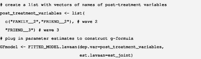
Appendix C.

R function to carry out steps B1 through B5 for the running example

To help researchers estimate the MSM using parametric g-formula in practice, we have developed a single R function FitMSM that carries out all the steps B1 to B5 described in the main text. In this section, we briefly describe the arguments of the function.

• trt.name: Prefix of the treatment variable names. Using our running example, if the treatment names in the dataset are LONELY__1 and LONELY__2, then trt.name=”LONELY__”.

• trt.T: Number of treatment timepoints. Using our running example, if there are two treatment timepoints, then trt.T = 2.

• baseline.names: Names of the covariates preceding the first treatment instance. These appear in the leftmost columns of the expanded data in Table 2 (under the column heading “Step B1”), and have identical values across all pseudo-copies. Using our running example, these would be the stable baseline covariates C (gender, race, age, and family SES (“INCOME”)), and pretreatment measurements of the time-varying variables L₁ (“FAMILY__1”), and Y₁ (“FRIEND__1”).

• post_treatment_variables: Names of the post-treatment variables modeled in the parametric g-formula, with the outcome of interest in the last entry. This is the same as the dep.var argument in the FITTED_MODEL.lavaan function above.

• regfit: Estimates of the regression models for the post-treatment variables from carrying out steps A1 and A2 above. Using our running example, regfit = GFmodel, where GFmodel was the object returned from the FITTED_MODEL.lavaan function.

• n.MC: Number of Monte Carlo pseudo-copies to be created. More pseudo-copies will yield more precise estimates. In our running example, n.MC = 100.

Applying this function to the observed data in our running example returns the point estimates of the causal parameters ψ₁ and ψ₂ in the MSM.

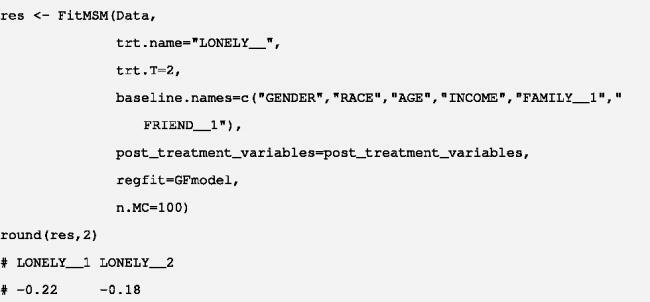
Appendix D.

Doubly robust variant

In this section, we describe how to include propensity score models in the estimation procedure above. Our proposal heuristically extends the doubly robust standardization method in Vansteelandt and Keiding (2011) for treatment at a single timepoint to the current setting of a time-varying treatment. Specifically, we will utilize inverse probability of treatment weights (IPW; Lunceford & Davidian, 2004), when fitting the regression models for the post-treatment variables in models (16) and (17).

Before introducing this extension, we briefly explain the motivation for supplementing the estimator of the parametric g-formula with IPW. IPW eliminates measured confounding by weighting the observed sample to be representative of a pseudo-population in which the covariate distributions are (approximately) similar, or “balanced,” across the treated and untreated groups (Thoemmes & Ong, 2015; Vandecandelaere et al., 2016; West et al., 2014). Vandecandelaere et al. (2016) describe a simple hypothetical example of how each observed individual contributes to the pseudopopulation. Therefore, when the sequential ignorability assumption holds, and the propensity score model is correctly specified, this pseudo-population has no confounder-treatment associations and is thus not subject to measured confounding (Vansteelandt & Keiding, 2011). The risks of biases due to model misspecification are reduced because valid causal effect estimates can be obtained if either the propensity score models, such as (D1) and (D2) below, or the regression models for the post-treatment variables, such as Equations (16)(16) $$\begin{array}{l}\mathrm{E}(Y_3|x_2,l_2,y_2,x_1,l_1,y_1,c)\\ ={\beta }_{y3,0}+{\beta }_{y3,x2}{x}_2+{\beta }_{y3,l2}{l}_2+{\beta }_{y3,y2}{y}_2+{\beta }_{y3,x2:l2}{x}_2{l}_2+{\beta }_{y3,x2:y2}{x}_2{y}_2+{\beta }_{y3,x1}{x}_1+{\beta }_{y3,l1}{l}_1+{\beta }_{y3,y1}{y}_1+{\beta }_{y3,c}c.\end{array}$$(16) and (17)(17) $$\begin{array}{l}\left[\begin{array}{c}{L}_2\\ Y_2\end{array}\right]\sim {\mathcal{N}}_2\left(\left[\begin{array}{c}{\mu }_{L_2|x_1,l_1,y_1,c}\\ {\mu }_{Y_2|x_1,l_1,y_1,c}\end{array}\right],{\Sigma }_{L_2,Y_2|x_1,l_1,y_1,c}\right);\\ {\mu }_{L_2|x_1,l_1,y_1,c}={\beta }_{l2,0}+{\beta }_{l2,x1}{x}_1+{\beta }_{l2,l1}{l}_1+{\beta }_{l2,y1}{y}_1+{\beta }_{l2,x1:l1}{x}_1{l}_1+{\beta }_{l2,x1:y1}{x}_1{y}_1+{\beta }_{l2,c}c,\\ {\mu }_{Y_2|x_1,l_1,y_1,c}={\beta }_{y2,0}+{\beta }_{y2,x1}{x}_1+{\beta }_{y2,l1}{l}_1+{\beta }_{y2,y1}{y}_1+{\beta }_{y2,x1:l1}{x}_1{l}_1+{\beta }_{y2,x1:y1}{x}_1{y}_1+{\beta }_{y2,c}c,\\ {\Sigma }_{L_2,Y_2|x_1,l_1,y_1,c}=\left[\begin{array}{cc}{\sigma }_{l2}^2& {\sigma }_{l2,y2}\\ {\sigma }_{l2,y2}& {\sigma }_{y2}^2\end{array}\right].\end{array}$$(17) in the main text, are correctly specified; see, e.g., Funk et al. (2011), Robins et al. (2007), Schafer and Kang (2008), and Vansteelandt and Keiding (2011) for more detailed and technical discussions about the double robustness property.⁸ In Appendix E, we empirically demonstrate the biases induced by an incorrectly specified outcome regression function, and the reduction in biases achieved by supplementing it with correctly specified propensity score models, in a simulation study.

Supplementing a regression model for the outcome or time-varying covariate with the (inverse) propensity scores has the added advantage of reducing the repercussions of relying solely on regression models, such as extrapolation bias and incoherence with the MSM, while reaping the benefits of regression-based adjustment, namely increased statistical efficiency (Vansteelandt et al., 2012; Vansteelandt & Keiding, 2011). We note that for treatment at a single timepoint, the doubly robust parametric g-formula approach described herein is identical to Vansteelandt and Keiding (2011), and follows the methodology for constructing the weighted regression estimator in Morgan and Winship (2015, Section 7.1). Similar approaches combining outcome regression functions and propensity score models for time-varying treatments have previously been applied in the epidemiological literature (Sudan et al., 2013; Thomson et al., 2022).

We now describe how to include propensity score models when estimating the parametric g-formula. We use the prefix “C” to designate each step of the doubly-robust procedure.

C1. For each treatment $X_t,t=1,2,$ in turn, fit a model for the propensity score, which is the conditional probability that an individual would have selected treatment at that time t given the pretreatment covariates (Rosenbaum & Rubin, 1983), to the observed data. In this paper, we use a logistic regression model given the covariates preceding X_t in the adjustment set ${\mathcal{C}}_t,$ which include the treatment history (at times before t), current and past time-varying variables (at times t or earlier), and baseline covariates (at t = 1). For example, for t = 1, a model with main effects for ($C,L_1,Y_1$) is:

(D1) $$\text{logit}\left\{\mathrm{E}(X_1|L_1,Y_1,C)\right\}={\alpha }_{1,0}+{\alpha }_{1,1}{L}_1+{\alpha }_{1,2}{Y}_1+{\alpha }_{1,3}C.$$(D1)

Similarly, for t = 2, a model with main effects for ($C,L_1,Y_1,L_2,Y_2$) is:

(D2) $$\begin{array}{c}\text{logit}\left\{\mathrm{E}(X_2|L_2,Y_2,X_1,L_1,Y_1,C)\right\}\\ \hspace{1em}={\alpha }_{2,0}+{\alpha }_{2,1}{L}_2+{\alpha }_{2,2}{Y}_2+{\alpha }_{2,3}{X}_1+{\alpha }_{2,4}{L}_1+{\alpha }_{2,5}{Y}_1+{\alpha }_{2,6}C.\end{array}$$(D2)

Calculate the MLEs of the coefficients.

C2. Calculate the predicted propensity scores specific to time t for each individual, denoted by P_t, by plugging in the MLEs for the coefficients in (D1) and (D2).

C3. Construct the time-specific inverse propensity score weights for each individual as:

$$W_t=\frac{X_t}{P_t}+\frac{1-X_t}{1-P_t},\hspace{1em}t=1,2.$$

The individual weight W_t is the inverse or reciprocal of the predicted probability of an individual’s observed treatment at time t, conditional on the measured covariates in the adjustment set ${\mathcal{C}}_t.$ We emphasize that each individual possesses a separate weight W_t for each distinct treatment timepoint t.

C4. In place of step A1, fit the regression model for the outcome (Equation (16)(16) $$\begin{array}{l}\mathrm{E}(Y_3|x_2,l_2,y_2,x_1,l_1,y_1,c)\\ ={\beta }_{y3,0}+{\beta }_{y3,x2}{x}_2+{\beta }_{y3,l2}{l}_2+{\beta }_{y3,y2}{y}_2+{\beta }_{y3,x2:l2}{x}_2{l}_2+{\beta }_{y3,x2:y2}{x}_2{y}_2+{\beta }_{y3,x1}{x}_1+{\beta }_{y3,l1}{l}_1+{\beta }_{y3,y1}{y}_1+{\beta }_{y3,c}c.\end{array}$$(16) ), but use the product of weights above $W_1{W}_2$ for each observation in the fitting procedure. For example, when using lavaan to fit the model, the weights can be readily incorporated using the “sampling.weights” argument. Following Fewell et al. (2004), Thoemmes and Ong (2015), and Vandecandelaere et al. (2016), the cumulative product of the weights is used because we are estimating the effects of both treatments X₁ and X₂ concurrently.

C5.Similarly, in place of step A2, fit the model (17) for the time-varying variables L₂ and Y₂ in step A2, but using the calculated weights W₁ for each observation. Because X₁ is the only treatment instance preceding L₂, only the weights W₁ corresponding to X₁ are used.

In other words, in the doubly-robust procedure, steps C1 to C5 are used instead of steps A1 and A2. The resulting fitted regression models can then be used to carry out steps B1 to B5 as described above to estimate the MSM. As in the previous procedure, nonparametric percentile bootstrap confidence intervals may be constructed by randomly resampling observations with replacement and repeating all the steps (C1 to C5, and B1 to B5) for each bootstrap sample.

Applying this doubly robust variant to the running example, the estimated effect of loneliness at timepoint 1 on friendship quality was ${\psi }_1=-0.25;95\%\text{CI}=(-0.39,-0.09),$ and of loneliness at timepoint 2 was ${\psi }_2=-0.20;95\%\text{CI}=(-0.34,-0.06).$ The effect estimates either without using any weights (as in the main text), or with the inverse probability weights (as with the doubly robust variance) were very similar. In practice, we encourage researchers to conduct sensitivity analyses to gauge the robustness of the MSM estimates to other plausible statistical models. This can be carried out by fitting different regression models, such as Equations (16)(16) $$\begin{array}{l}\mathrm{E}(Y_3|x_2,l_2,y_2,x_1,l_1,y_1,c)\\ ={\beta }_{y3,0}+{\beta }_{y3,x2}{x}_2+{\beta }_{y3,l2}{l}_2+{\beta }_{y3,y2}{y}_2+{\beta }_{y3,x2:l2}{x}_2{l}_2+{\beta }_{y3,x2:y2}{x}_2{y}_2+{\beta }_{y3,x1}{x}_1+{\beta }_{y3,l1}{l}_1+{\beta }_{y3,y1}{y}_1+{\beta }_{y3,c}c.\end{array}$$(16) and (17)(17) $$\begin{array}{l}\left[\begin{array}{c}{L}_2\\ Y_2\end{array}\right]\sim {\mathcal{N}}_2\left(\left[\begin{array}{c}{\mu }_{L_2|x_1,l_1,y_1,c}\\ {\mu }_{Y_2|x_1,l_1,y_1,c}\end{array}\right],{\Sigma }_{L_2,Y_2|x_1,l_1,y_1,c}\right);\\ {\mu }_{L_2|x_1,l_1,y_1,c}={\beta }_{l2,0}+{\beta }_{l2,x1}{x}_1+{\beta }_{l2,l1}{l}_1+{\beta }_{l2,y1}{y}_1+{\beta }_{l2,x1:l1}{x}_1{l}_1+{\beta }_{l2,x1:y1}{x}_1{y}_1+{\beta }_{l2,c}c,\\ {\mu }_{Y_2|x_1,l_1,y_1,c}={\beta }_{y2,0}+{\beta }_{y2,x1}{x}_1+{\beta }_{y2,l1}{l}_1+{\beta }_{y2,y1}{y}_1+{\beta }_{y2,x1:l1}{x}_1{l}_1+{\beta }_{y2,x1:y1}{x}_1{y}_1+{\beta }_{y2,c}c,\\ {\Sigma }_{L_2,Y_2|x_1,l_1,y_1,c}=\left[\begin{array}{cc}{\sigma }_{l2}^2& {\sigma }_{l2,y2}\\ {\sigma }_{l2,y2}& {\sigma }_{y2}^2\end{array}\right].\end{array}$$(17) , and propensity score models, such as (D1) and (D2), then assessing whether the resulting causal effect estimates differ substantively.

Appendix E.

Simulation study

We conducted a small Monte Carlo simulation study to empirically illustrate that, in the presence of treatment-dependent confounding, estimates of time-varying treatments are biased using standard regression, but unbiased using the parametric g-formula. The study was conducted under the setting shown in Figure 1, but with only a single end-of-study outcome Y in the final timepoint (i.e., without the earlier outcomes Y₁ or Y₂). There was a nonrandomized binary treatment measured at the first two timepoints (X₁ and X₂), an outcome measured at the end of the study (Y), a treatment-dependent confounder measured at both treatment timepoints (L₁ and L₂), and a single time-invariant confounder C. In the first setting, we generated each simulated dataset such that the outcome (Y) was based on a linear model with only main effects for the predictors. The same (hence correctly specified) model was then fitted to each simulated dataset. We used this setting to demonstrate the biases which can arise from using standard regression methods to estimate the effect of X₁ on Y while adjusting (or statistically controlling) for the intervening time-varying covariate L₂. In the second setting, we generated Y based on a model with complicated nonlinear functions of the predictors. We then fitted to each simulated dataset the same linear regression model as in the previous setting so that the outcome model was incorrectly specified; however, the propensity score model was correctly specified. We used the second setting to demonstrate the proposed double robust estimator.

Data-generating processes

For each setting, each simulated dataset was generated as follows. $$\begin{array}{c}U\sim \mathcal{N}(0,1)\\ C\sim \text{Exponential}(\lambda =2);\mathrm{E}(C)=0.5\\ L_1=2U+{ϵ}_{l1};{ϵ}_{l1}\sim \mathcal{N}(0,1)\\ X_1\sim \text{Bernoulli}\left\{\frac{\hspace{0.17em}\mathrm{\text{exp}}\hspace{0.17em}(0.1L_1+0.1C)}{1+\hspace{0.17em}\mathrm{\text{exp}}\hspace{0.17em}(0.1L_1+0.1C)}\right\}\end{array}$$

The variable U was a time-invariant common cause of the covariates $L_t,t=1,2,$ and outcome Y; U was hidden from the observed data to induce unmeasured confounding among these variables. The initial treatment X₁ affected the time-varying covariate L₂, which subsequently affected the later treatment X₂. $$\begin{array}{c}{L}_2=L_1+C+(X_1-0.5)+2U+{ϵ}_{l2};{ϵ}_{l2}\sim \mathcal{N}(0,1)\\ X_2\sim \text{Bernoulli}\left\{\frac{\hspace{0.17em}\mathrm{\text{exp}}\hspace{0.17em}(0.3L_2+0.1C)}{1+\hspace{0.17em}\mathrm{\text{exp}}\hspace{0.17em}(0.3L_2+0.1C)}\right\}\\ Y=b_y(L_1,C,U)+{\psi }_2{X}_2+0.2X_1+(-0.1)L_2+4U+{ϵ}_y;{ϵ}_y\sim \mathcal{N}(0,1).\end{array}$$ The outcome was affected directly by both treatments (X₁ and X₂) and indirectly by the first treatment X₁ via the intervening time-varying covariate L₂. In other words, the direct effect of X₁ on Y which did not intersect L₂ was 0.2, whereas the indirect effect via L₂ was $(-0.1)\times 1$ (i.e., the product of the coefficients of L₂ on Y, and X₁ on L₂, respectively). Hence, the average causal effects of X₁ and X₂ on Y were, respectively, ${\psi }_1=0.2+(-0.1)=0.1,$ and ${\psi }_2=0.2.$

In the first setting, we set the functions of the baseline covariates in the data-generating model for Y as $b_y(L_1,C,U)=L_1+C,$ so it depended only on the main effects of the predictors. In the second setting, these functions were: $$b_y(L_1,C,U)=\left|L1\right|\hspace{0.17em}\mathrm{\text{log}}\hspace{0.17em}(C)+1\mathrm{}\left(U<0\right){(C-0.5)}^2+1\mathrm{}\left(U\ge 0\right)1\mathrm{}\left(L_1<0\right).$$

The outcomes Y in the second setting were thus generated using nonlinear and complex functions of the predictors so that a fitted model with only main effects for the predictors would be incorrectly specified.

Estimators under comparison

We considered three different estimators of ψ₁ and ψ₂ for each simulated dataset. We assumed only main effects for the predictors in the propensity score models and the regression models for the outcome and time-varying covariate.

1. A single regression model for the outcome Y, given all causally and temporally preceding variables.

   

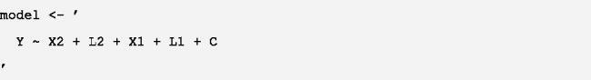
   We used the coefficients of X₂ and X₁ in the above model as estimators of ψ₂, and ψ₁, respectively. We will refer to this estimator as “Single regression.” Such an approach is routinely adopted for simultaneously estimating different lagged effects of treatment on the same outcome. Because this regression model was identical to the outcome model in the following parametric g-formula estimator, the estimator of ψ₂ using both these methods would be identical. But the estimators of ψ₁ would differ due to how the time-varying covariate L₂ is handled.⁹

2. The parametric g-formula was applied using only regression models for the time-varying covariate and outcome. No propensity scores were used. This estimator was used to: (i) evaluate its statistical efficiency under a correctly specified outcome model (in the first setting) relative to the doubly robust variant; and (ii) to illustrate how when the outcome model is incorrectly specified – it was not weighted by the inverse propensity scores – the approach can lead to biased estimators (in the second setting). We fitted the following models simultaneously as:

   

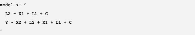
   We then fitted the MSM in Equation (15)(15) $${\mathrm{E}}_{(X_1,X_2)\leftarrow (x_1,x_2)}(Y_3)={\psi }_0+{\psi }_1{x}_1+{\psi }_2{x}_2.$$(15) by carrying out steps B1 to B5 as described above.

3. The parametric g-formula was then estimated using the doubly robust (“DR”) variant. We first fitted the propensity score models stated in (D1) and (D2) of Appendix D, then calculated the IPWs W₁ and W₂. We then separately fitted the regression models for L₂ and Y using these weights. First, the model for the time-varying covariate L₂, which included treatment only at time 1 and was thus weighted by the inverse propensity score W₁, can be fitted as follows:

   

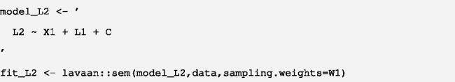
   Next, the model for the outcome Y, which included both treatments at times 1 and 2 and thus weighted by the inverse of the product of propensity scores $W_1{W}_2,$ was:

   

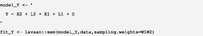
   Finally, we fitted the MSM in Equation (15)(15) $${\mathrm{E}}_{(X_1,X_2)\leftarrow (x_1,x_2)}(Y_3)={\psi }_0+{\psi }_1{x}_1+{\psi }_2{x}_2.$$(15) by carrying out steps B1 to B5 as described above.

Results

The results for 5000 simulated datasets, each with a sample size of 1000, under each setting, are shown in Table E1.¹⁰ In both settings, standard regression failed to produce unbiased estimates of ψ₁ (the treatment effect of X₁ on Y) due to inappropriate adjustment for the time-varying covariate L₂ within the same regression model.¹¹ Using the parametric g-formula with only regression models for post-treatment variables L₂ and Y yielded unbiased estimates of both ψ₁ and ψ₂ when the fitted models were correctly specified, as in the first setting. Furthermore, in this setting, this estimator was more precise (with a lower RMSE) than the doubly robust variant. In the second setting, the estimates of ψ₁ and ψ₂ were (slightly) biased when the fitted regression models were incorrectly specified. In contrast, the doubly robust variant of the parametric g-formula was unbiased for the time-varying treatment effects in both settings, notwithstanding the misspecified outcome model in the second setting.

Table E1. Empirical biases of different estimators of the causal effects ψ₁ and ψ₂.

		Mean		Bias		ESE		RMSE
DG models	Estimation method	ψ 1	ψ2	ψ1	ψ2	ψ1	ψ2	ψ1	ψ2
Linear	Single regression	−0.25	0.20	−0.35	0.00	0.08	0.09	0.36	0.09
Linear	Parametric g-formula	0.10	0.20	−0.00	0.00	0.08	0.09	0.08	0.09
Linear	Parametric g-formula (DR)	0.10	0.20	−0.00	0.00	0.10	0.10	0.10	0.10
Nonlinear	Single regression	−0.27	0.23	−0.37	0.03	0.21	0.20	0.43	0.20
Nonlinear	Parametric g-formula	0.09	0.23	−0.01	0.03	0.20	0.20	0.20	0.20
Nonlinear	Parametric g-formula (DR)	0.10	0.19	0.00	−0.01	0.32	0.33	0.32	0.33

Notes. “DG Models” = Data-generating Models; “DR” = doubly robust; ${\psi }_1=$ average causal effect of X₁ on Y, with a true value of 0.1; ${\psi }_2=$ average causal effect of X₂ on Y, with a true value of 0.2. In addition to the mean empirical estimates and the empirical biases, standard errors (“ESE”’) and root mean squared errors (“RMSE”) were also calculated. All results were rounded to two decimal places.

References

- Ahern, J. (2018). Start with the “C-Word,” follow the roadmap for causal inference. American Journal of Public Health, 108(5), 621–621. https://doi.org/10.2105/AJPH.2018.304358
- Andersen, H. K. (2022). Equivalent approaches to dealing with unobserved heterogeneity in cross-lagged panel models? investigating the benefits and drawbacks of the latent curve model with structured residuals and the random intercept cross-lagged panel model. Psychological Methods, 27(5), 730–751. https://doi.org/10.1037/met0000285
- Arbuckle, J. L. (2019). Amos (Version 26.0) [computer program]. IBM SPSS. SPSS Inc.
- Boker, S., Neale, M., Maes, H., Wilde, M., Spiegel, M., Brick, T., Spies, J., Estabrook, R., Kenny, S., Bates, T., Mehta, P., & Fox, J. (2011). OpenMx: An open source extended structural equation modeling framework. Psychometrika, 76(2), 306–317. https://doi.org/10.1007/s11336-010-9200-6
- Bray, B. C., Almirall, D., Zimmerman, R. S., Lynam, D., & Murphy, S. A. (2006). Assessing the total effect of time-varying predictors in prevention research. Prevention Science, 7(1), 1–17. https://doi.org/10.1007/s11121-005-0023-0
- Breskin, A., Cole, S. R., & Westreich, D. (2018). Exploring the subtleties of inverse probability weighting and marginal structural models. Epidemiology, 29(3), 352–355. https://doi.org/10.1097/EDE.0000000000000813
- Danaei, G., Pan, A., Hu, F. B., & Hernán, M. A. (2013). Hypothetical midlife interventions in women and risk of type 2 diabetes. Epidemiology, 24(1), 122–128. https://doi.org/10.1097/EDE.0b013e318276c98a
- Daniel, R. M. (2018). G-computation formula. In N. Balakrishnan, T. Colton, B. Everitt, W. Piegorsch, F. Ruggeri, & J. Teugels (Eds.), Wiley statsref: Statistics reference online (pp. 1–10). John Wiley & Sons, Ltd.
- Daniel, R. M., Cousens, S., De Stavola, B., Kenward, M. G., & Sterne, J. A. C. (2013). Methods for dealing with time-dependent confounding. Statistics in Medicine, 32(9), 1584–1618. https://doi.org/10.1002/sim.5686
- Daniel, R. M., De Stavola, B. L., & Cousens, S. N. (2011). Gformula: Estimating causal effects in the presence of time-varying confounding or mediation using the g-computation formula. The Stata Journal, 11(4), 479–517. https://doi.org/10.1177/1536867X1201100401
- Digitale, J. C., Martin, J. N., & Glymour, M. M. (2022). Tutorial on directed acyclic graphs. Journal of Clinical Epidemiology, 142, 264–267. https://doi.org/10.1016/j.jclinepi.2021.08.001
- Edwards, J. K., McGrath, L. J., Buckley, J. P., Schubauer-Berigan, M. K., Cole, S. R., & Richardson, D. B. (2014). Occupational radon exposure and lung cancer mortality: Estimating intervention effects using the parametric g-formula. Epidemiology, 25(6), 829–834. https://doi.org/10.1097/EDE.0000000000000164
- Efron, B., & Tibshirani, R. J. (1994). An introduction to the bootstrap. Chapman & Hall\CRC.
- Elwert, F. (2013). Graphical causal models. In S. L. Morgan (Ed.), Handbook of causal analysis for social research (pp. 245–273). Springer. https://doi.org/10.1007/978-94-007-6094-3_13
- Elwert, F., & Winship, C. (2014). Endogenous selection bias: The problem of conditioning on a collider variable. Annual Review of Sociology, 40(1), 31–53. https://doi.org/10.1146/annurev-soc-071913-043455
- Enders, C. K. (2022). Applied missing data analysis (2nd ed.). The Guilford Press.
- Fewell, Z., Hernán, M. A., Wolfe, F., Tilling, K., Choi, H., & Sterne, J. A. C. (2004). Controlling for time-dependent confounding using marginal structural models. Stata Journal, 4(4), 402–420.
- Funk, M. J., Westreich, D., Wiesen, C., Stürmer, T., Brookhart, M. A., & Davidian, M. (2011). Doubly robust estimation of causal effects. American Journal of Epidemiology, 173(7), 761–767. https://doi.org/10.1093/aje/kwq439
- Gill, R. D., & Robins, J. M. (2001). Causal inference for complex longitudinal data: The continuous case. The Annals of Statistics, 29(6), 1785–1811. https://doi.org/10.1214/aos/1015345962
- Gische, C., West, S. G., & Voelkle, M. C. (2021). Forecasting causal effects of interventions versus predicting future outcomes. Structural Equation Modeling: A Multidisciplinary Journal, 28(3), 475–492. https://doi.org/10.1080/10705511.2020.1780598
- Gollob, H. F., & Reichardt, C. S. (1987). Taking account of time lags in causal models. Child Development, 58(1), 80–92. https://doi.org/10.2307/1130293
- Greenland, S., Pearl, J., & Robins, J. M. (1999). Causal diagrams for epidemiologic research. Epidemiology, 10(1), 37–48. https://doi.org/10.1097/00001648-199901000-00008
- Griffith, G. J., Morris, T. T., Tudball, M. J., Herbert, A., Mancano, G., Pike, L., Sharp, G. C., Sterne, J., Palmer, T. M., Davey Smith, G., Tilling, K., Zuccolo, L., Davies, N. M., & Hemani, G. (2020). Collider bias undermines our understanding of covid-19 disease risk and severity. Nature Communications, 11(1), 5749. https://doi.org/10.1038/s41467-020-19478-2
- Grosz, M. P., Rohrer, J. M., & Thoemmes, F. (2020). The taboo against explicit causal inference in nonexperimental psychology. Perspectives on Psychological Science, 15(5), 1243–1255. https://doi.org/10.1177/1745691620921521
- Hatcher, L. (1996). Using SAS®PROC CALIS for path analysis: An introduction. Structural Equation Modeling: A Multidisciplinary Journal, 3(2), 176–192. https://doi.org/10.1080/10705519609540037
- Hernán, M. A. (2018). The C-Word: Scientific euphemisms do not improve causal inference from observational data. American Journal of Public Health, 108(5), 616–619. https://doi.org/10.2105/AJPH.2018.304337
- Hernán, M. A., & Robins, J. M. (2020). Causal inference: What if. Chapman & Hall\CRC.
- Hong, G., & Raudenbush, S. W. (2006). Evaluating kindergarten retention policy: A case study of causal inference for multilevel observational data. Journal of the American Statistical Association, 101(475), 901–910. https://doi.org/10.1198/016214506000000447
- Imbens, G. W., & Rubin, D. B. (2015). Causal inference in statistics, social, and biomedical sciences. Cambridge University Press.
- Keil, A. P., Edwards, J. K., Richardson, D. B., Naimi, A. I., & Cole, S. R. (2014). The parametric g-formula for time-to-event data: Intuition and a worked example. Epidemiology, 25(6), 889–897. https://doi.org/10.1097/EDE.0000000000000160
- Kennedy, T. M., Kennedy, E. H., & Ceballo, R. (2022). Marginal structural models for estimating the longitudinal effects of community violence exposure on youths’ internalizing and externalizing symptoms. Psychological Trauma: Theory, Research, Practice, and Policy, 15(6), 906–916. https://doi.org/10.1037/tra0001398
- Keogh, R. H., Daniel, R. M., VanderWeele, T. J., & Vansteelandt, S. (2017). Analysis of longitudinal studies with repeated outcome measures: Adjusting for time-dependent confounding using conventional methods. American Journal of Epidemiology, 187(5), 1085–1092. https://doi.org/10.1093/aje/kwx311
- Kim, Y., & Steiner, P. M. (2020). Causal graphical views of fixed effects and random effects models. British Journal of Mathematical and Statistical Psychology, 74(2), 165–183.
- Kühhirt, M., & Klein, M. (2018). Early maternal employment and children’s vocabulary and inductive reasoning ability: A dynamic approach. Child Development, 89(2), e91–e106. https://doi.org/10.1111/cdev.12796
- Lee, T., & Shi, D. (2021). A comparison of full information maximum likelihood and multiple imputation in structural equation modeling with missing data. Psychological Methods, 26(4), 466–485. https://doi.org/10.1037/met0000381
- Leyrat, C., Carpenter, J. R., Bailly, S., & Williamson, E. J. (2021). Common methods for handling missing data in marginal structural models: What works and why. American Journal of Epidemiology, 190(4), 663–672. https://doi.org/10.1093/aje/kwaa225
- Loh, W. W. (2024). Estimating curvilinear time-varying treatment effects: Combining g-estimation of structural nested mean models with time-varying effect models for longitudinal causal inference. Psychological Methods. https://doi.org/10.1037/met0000637
- Loh, W. W., & Ren, D. (2023a). A tutorial on causal inference in longitudinal data with time-varying confounding using g-estimation. Advances in Methods and Practices in Psychological Science, 6(3). https://doi.org/10.1177/25152459231174029
- Loh, W. W., & Ren, D. (2023b). Estimating time-varying treatment effects in longitudinal studies. Psychological Methods. Advance online publication. https://doi.org/10.1037/met0000574
- Loh, W. W., & Ren, D. (2023c). The unfulfilled promise of longitudinal designs for causal inference. Collabra: Psychology, 9(1), 89142. https://doi.org/10.1525/collabra.89142
- Lüdtke, O., & Robitzsch, A. (2022). A comparison of different approaches for estimating cross-lagged effects from a causal inference perspective. Structural Equation Modeling: A Multidisciplinary Journal, 29(6), 888–907. https://doi.org/10.1080/10705511.2022.2065278
- Lunceford, J. K., & Davidian, M. (2004). Stratification and weighting via the propensity score in estimation of causal treatment effects: A comparative study. Statistics in Medicine, 23(19), 2937–2960. https://doi.org/10.1002/sim.1903
- Mathisen, J., Nguyen, T.-L., Jensen, J. H., Mehta, A. J., Rugulies, R., & Rod, N. H. (2022). Impact of hypothetical improvements in the psychosocial work environment on sickness absence rates: A simulation study. European Journal of Public Health, 32(5), 716–722. https://doi.org/10.1093/eurpub/ckac109
- McGrath, S., Lin, V., Zhang, Z., Petito, L. C., Logan, R. W., Hernán, M. A., & Young, J. G. (2020). gfoRmula: An R package for estimating the effects of sustained treatment strategies via the parametric g-formula. Patterns, 1(3), 10008. https://doi.org/10.1016/j.patter.2020.100008
- Meng, X.-L. (1994). Multiple-imputation inferences with uncongenial sources of input. Statistical Science, 9(4), 538–558.
- Moodie, E. E. M., & Stephens, D. A. (2010). Using directed acyclic graphs to detect limitations of traditional regression in longitudinal studies. International Journal of Public Health, 55(6), 701–703. https://doi.org/10.1007/s00038-010-0184-x
- Morgan, S. L., & Winship, C. (2015). Counterfactuals and causal inference. Cambridge University Press.
- Muthén, L. K., & Muthén, B. (1998–2017). Mplus user’s guide: Statistical analysis with latent variables (8th ed.). Muthén & Muthén.
- Naimi, A. I., Cole, S. R., & Kennedy, E. H. (2016). An introduction to g methods. International Journal of Epidemiology, 46(2), 756–762. https://doi.org/10.1093/ije/dyw323
- Pearl, J. (2009). Causality: Models, reasoning and inference (2nd ed.). Cambridge University Press.
- Pearl, J. (2010). On the consistency rule in causal inference: Axiom, definition, assumption, or theorem? Epidemiology, 21(6), 872–875. https://doi.org/10.1097/EDE.0b013e3181f5d3fd
- Pearl, J., Glymour, M., & Jewell, N. P. (2016). Causal inference in statistics: A primer. John Wiley & Sons Ltd.
- Petersen, M. L., Porter, K. E., Gruber, S., Wang, Y., & Van der Laan, M. J. (2012). Diagnosing and responding to violations in the positivity assumption. Statistical Methods in Medical Research, 21(1), 31–54. https://doi.org/10.1177/0962280210386207
- Petersen, M. L., Schwab, J., Gruber, S., Blaser, N., Schomaker, M., & Van der Laan, M. J. (2014). Targeted maximum likelihood estimation for dynamic and static longitudinal marginal structural working models. Journal of Causal Inference, 2(2), 147–185. https://doi.org/10.1515/jci-2013-0007
- Potthoff, R. F., Tudor, G. E., Pieper, K. S., & Hasselblad, V. (2006). Can one assess whether missing data are missing at random in medical studies? Statistical Methods in Medical Research, 15(3), 213–234. https://doi.org/10.1191/0962280206sm448oa
- R Core Team. (2021). R: A Language and Environment for Statistical Computing. R Foundation for Statistical Computing.
- Robert, C. P., & Casella, G. (2010). Monte Carlo integration (pp. 61–88). Springer.
- Robins, J. M. (1986). A new approach to causal inference in mortality studies with a sustained exposure period—Application to control of the healthy worker survivor effect. Mathematical Modelling, 7(9), 1393–1512. https://doi.org/10.1016/0270-0255(86)90088-6
- Robins, J. M. (1997). Causal inference from complex longitudinal data. In M. Berkane (Ed.), Latent variable modeling and applications to causality (pp. 69–117). Springer.
- Robins, J. M., Greenland, S., & Hu, F.-C. (1999). Estimation of the causal effect of a time-varying exposure on the marginal mean of a repeated binary outcome. Journal of the American Statistical Association, 94(447), 687–700. https://doi.org/10.1080/01621459.1999.10474168
- Robins, J. M., Hernán, M. A., & Brumback, B. (2000). Marginal structural models and causal inference in epidemiology. Epidemiology, 11(5), 550–560. https://doi.org/10.1097/00001648-200009000-00011
- Robins, J. M., Sued, M., Lei-Gomez, Q., & Rotnitzky, A. (2007). Comment: Performance of double-robust estimators when “inverse probability” weights are highly variable. Statistical Science, 22(4), 544–559. https://doi.org/10.1214/07-STS227D
- Rohrer, J. M. (2018). Thinking clearly about correlations and causation: Graphical causal models for observational data. Advances in Methods and Practices in Psychological Science, 1(1), 27–42. https://doi.org/10.1177/2515245917745629
- Rosenbaum, P. R. (1984). The consequences of adjustment for a concomitant variable that has been affected by the treatment. Journal of the Royal Statistical Society. Series A (General), 147(5), 656–666. https://doi.org/10.2307/2981697
- Rosenbaum, P. R., & Rubin, D. B. (1983). The central role of the propensity score in observational studies for causal effects. Biometrika, 70(1), 41–55. https://doi.org/10.1093/biomet/70.1.41
- Rosseel, Y. (2012). lavaan: An R package for structural equation modeling. Journal of Statistical Software, 48(2), 1–36. https://doi.org/10.18637/jss.v048.i02
- Rudolph, J. E., Benkeser, D., Kennedy, E. H., Schisterman, E. F., & Naimi, A. I. (2022). Estimation of the average causal effect in longitudinal data with time-varying exposures: The challenge of nonpositivity and the impact of model flexibility. American Journal of Epidemiology, 191(11), 1962–1969. https://doi.org/10.1093/aje/kwac136
- Schafer, J. L., & Kang, J. (2008). Average causal effects from nonrandomized studies: A practical guide and simulated example. Psychological Methods, 13(4), 279–313. https://doi.org/10.1037/a0014268
- Schisterman, E. F., Cole, S. R., & Platt, R. W. (2009). Overadjustment bias and unnecessary adjustment in epidemiologic studies. Epidemiology, 20(4), 488–495. https://doi.org/10.1097/EDE.0b013e3181a819a1
- Shpitser, I., & Pearl, J. (2006). Identification of conditional interventional distributions. In R. Dechter & T. S. Richardson (Eds.,) Proceedings of the Twenty-Second Conference on Uncertainty in Artificial Intelligence, UAI’06 (pp. 437–444). AUAI Press.
- Snowden, J. M., Rose, S., & Mortimer, K. M. (2011). Implementation of G-computation on a simulated data set: Demonstration of a causal inference technique. American Journal of Epidemiology, 173(7), 731–738. https://doi.org/10.1093/aje/kwq472
- Spirtes, P., Glymour, C., & Scheines, R. (2001). Causation, prediction, and search (2nd ed.). The MIT Press.
- Stavrova, O., & Ren, D. (2023). Alone in a crowd: Is social contact associated with less psychological pain of loneliness in everyday life? Journal of Happiness Studies, 24(5), 1841–1860. https://doi.org/10.1007/s10902-023-00661-3
- Steiner, P. M., Cook, T. D., Shadish, W. R., & Clark, M. H. (2010). The importance of covariate selection in controlling for selection bias in observational studies. Psychological Methods, 15(3), 250–267. https://doi.org/10.1037/a0018719
- Sudan, M., Kheifets, L., Arah, O. A., & Olsen, J. (2013). Cell phone exposures and hearing loss in children in the Danish national birth cohort. Paediatric and Perinatal Epidemiology, 27(3), 247–257. https://doi.org/10.1111/ppe.12036
- Suk, H. W., West, S. G., Fine, K. L., & Grimm, K. J. (2019). Nonlinear growth curve modeling using penalized spline models: A gentle introduction. Psychological Methods, 24(3), 269–290. https://doi.org/10.1037/met0000193
- Taubman, S. L., Robins, J. M., Mittleman, M. A., & Hernán, M. A. (2009). Intervening on risk factors for coronary heart disease: An application of the parametric g-formula. International Journal of Epidemiology, 38(6), 1599–1611. https://doi.org/10.1093/ije/dyp192
- Thoemmes, F. J., & Ong, A. D. (2015). A primer on inverse probability of treatment weighting and marginal structural models. Emerging Adulthood, 4(1), 40–59. https://doi.org/10.1177/2167696815621645
- Thoemmes, F. J., & West, S. G. (2011). The use of propensity scores for nonrandomized designs with clustered data. Multivariate Behavioral Research, 46(3), 514–543. https://doi.org/10.1080/00273171.2011.569395
- Thomson, R. M., Kopasker, D., Leyland, A., Pearce, A., & Katikireddi, S. V. (2022). Effects of poverty on mental health in the UK working-age population: Causal analyses of the UK household longitudinal study. International Journal of Epidemiology, 52(2), 512–522. https://doi.org/10.1093/ije/dyac226
- Usami, S., Murayama, K., & Hamaker, E. L. (2019). A unified framework of longitudinal models to examine reciprocal relations. Psychological Methods, 24(5), 637–657. https://doi.org/10.1037/met0000210
- Vandecandelaere, M., Vansteelandt, S., De Fraine, B., & Van Damme, J. (2016). Time-varying treatments in observational studies: Marginal structural models of the effects of early grade retention on math achievement. Multivariate Behavioral Research, 51(6), 843–864. https://doi.org/10.1080/00273171.2016.1155146
- VanderWeele, T. J. (2009). On the distinction between interaction and effect modification. Epidemiology, 20(6), 863–871. https://doi.org/10.1097/EDE.0b013e3181ba333c
- VanderWeele, T. J., Hawkley, L. C., Thisted, R. A., & Cacioppo, J. T. (2011). A marginal structural model analysis for loneliness: Implications for intervention trials and clinical practice. Journal of Consulting and Clinical Psychology, 79(2), 225–235. https://doi.org/10.1037/a0022610
- VanderWeele, T. J., Jackson, J. W., & Li, S. (2016). Causal inference and longitudinal data: A case study of religion and mental health. Social Psychiatry and Psychiatric Epidemiology, 51(11), 1457–1466. https://doi.org/10.1007/s00127-016-1281-9
- VanderWeele, T. J., Mathur, M. B., & Chen, Y. (2020). Outcome-wide longitudinal designs for causal inference: A new template for empirical studies. Statistical Science, 35(3), 437–466. https://doi.org/10.1214/19-STS728
- Vansteelandt, S., Bekaert, M., & Claeskens, G. (2012). On model selection and model misspecification in causal inference. Statistical Methods in Medical Research, 21(1), 7–30. https://doi.org/10.1177/0962280210387717
- Vansteelandt, S., & Keiding, N. (2011). Invited commentary: G-computation–lost in translation? American Journal of Epidemiology, 173(7), 739–742. https://doi.org/10.1093/aje/kwq474
- West, S. G., Aiken, L. S., & Krull, J. L. (1996). Experimental personality designs: Analyzing categorical by continuous variable interactions. Journal of Personality, 64(1), 1–48. https://doi.org/10.1111/j.1467-6494.1996.tb00813.x
- West, S. G., Cham, H., Thoemmes, F., Renneberg, B., Schulze, J., & Weiler, M. (2014). Propensity scores as a basis for equating groups: Basic principles and application in clinical treatment outcome research. Journal of Consulting and Clinical Psychology, 82(5), 906–919. https://doi.org/10.1037/a0036387
- Westreich, D., Cole, S. R., Young, J. G., Palella, F., Tien, P. C., Kingsley, L., Gange, S. J., & Hernán, M. A. (2012). The parametric g-formula to estimate the effect of highly active antiretroviral therapy on incident AIDS or death. Statistics in Medicine, 31(18), 2000–2009. https://doi.org/10.1002/sim.5316
- Wright, S. (1934). The method of path coefficients. The Annals of Mathematical Statistics, 5(3), 161–215. https://doi.org/10.1214/aoms/1177732676
- Young, J. G., Cain, L. E., Robins, J. M.’ O'Reilly, E. J., & Hernán, M. A. (2011). Comparative effectiveness of dynamic treatment regimes: An application of the parametric g-formula. Statistics in Biosciences, 3(1), 119–143. https://doi.org/10.1007/s12561-011-9040-7
- Zhang, Y., Young, J. G., Thamer, M., & Hernán, M. A. (2018). Comparing the effectiveness of dynamic treatment strategies using electronic health records: An application of the parametric g-formula to anemia management strategies. Health Services Research, 53(3), 1900–1918. https://doi.org/10.1111/1475-6773.12718
- Zimmerman, M. A. (2014). Flint Michigan Adolescent Study (FAS): A longitudinal study of school dropout and substance use, 1994-1997.