Cost-benefit analysis blueprint for regional weed management: Nassella neesiana (Chilean needle grass) as a case study

Abstract

We describe a bio-economic model for Nassella neesiana (Chilean needle grass) that estimates the net benefit of a containment programme for the weed in Canterbury as the difference between the cost of containment and the costs incurred over time should the weed spread within sheep and beef pastoral systems. Logistic spread is assumed with the maximum area that could be invaded (772,080 ha) determined by constraining a climate niche model for the weed to susceptible farm system types within productive land use capability classes. The current size of the invaded area (80 ha) was determined by field observations in Canterbury in 2008, and the spread rate (201 years to 90% saturation) was derived from observations in the adjacent Marlborough region. With these assumptions, and discounting at 8% per year over 100 years, the net benefit is negative NZ$173,178 ($83,900–$257,078) and containment would not be economically worthwhile. However, the net benefit is positive over a range of lower discount rates and higher spread rates, revealing a need for robust estimates of these parameters. The model presented here provides a generic blueprint for meeting the requirements of the Biosecurity Act with respect to evaluating proposed regional weed management programmes.

Keywords:

• logistic model
• New Zealand Biosecurity Act 1993
• social discount rate
• weed control
• weed spread

Introduction

Weed species in New Zealand that have become widespread, and as a consequence are not considered to be a biosecurity threat, are managed on a voluntary basis by affected landowners or occupiers. Examples of such weeds are the many species that are common in arable crops and pastures (Bourdôt et al. 1998, 2007). By contrast, the management of established species that are of limited current distribution but have potential to spread and affect the economy, the environment, human health or sociocultural well-being, is provided for under the Biosecurity Act 1993 (Ministry for Primary Industries 2014). Reform of the Act in 2012 resulted in a number of changes to New Zealand's biosecurity system, many aimed at enabling nationally consistent information for decision-making (Ministry for Primary Industries 2013). For example, under the Act, weeds may be managed under a national or a regional pest management plan, a pathway management plan, or a small-scale management programme, and individual species programmes within these plans are to be classified, according to their intended outcome, as either ‘exclusion’, ‘eradication’, ‘progressive containment’ or ‘sustained control’ (Ministry for Primary Industries 2014).

The Biosecurity Act requires that ‘for each subject (e.g. a weed species), the benefits of the plan outweigh the costs, after taking account of the likely consequences of inaction or other courses of action’ and ‘that, for each subject, persons who are required, as a group, to meet directly any or all of the costs of implementing the plan, would accrue, as a group, benefits outweighing the costs’ (Ministry for Primary Industries 2014). To meet these requirements the agency proposing the plan, typically a regional council, must undertake a cost-benefit analysis for the proposed management of each species in the plan. Historically, cost-benefit analyses have often not been conducted or are reported in variable forms with important details missing (Ministry for Primary Industries 2013). Key elements of cost-benefit analyses for weed control programmes under the Act have been proposed (Giera & Bell 2009) and encompass: defining the problem and desired outcome; defining the control options; specifying a baseline scenario; estimating control costs; identifying the benefits of control; quantifying the magnitude of the benefits; appropriate discounting of future costs and benefits; consideration of any intangible costs; sensitivity analysis to account for risk and uncertainty; and reporting.

Here we present a model for determining the net benefit of a ‘containment’ programme for the invasive pelt-damaging grass weed Nassella neesiana (Chilean needle grass) in the Canterbury region of New Zealand. The goal is to contain the weed to its currently occupied area. The species, well-established and problematic in dry-land sheep and beef hill pastures in the Hawkes Bay and Marlborough regions of New Zealand (Bourdôt et al. 2010b) and in grasslands in the Northern Tablelands of New South Wales and the Volcanic Plain of Victoria, Australia (McLaren et al. 1998; Snell et al. 2007), was discovered as a localised infestation in a pasture in north Canterbury in 2008. Hitherto unknown in the region, community concern resulted in the species being recommended for inclusion in the Canterbury Regional Pest Management Plan to prevent its wider spread (via animals, water, machinery, hay, grain) and pastoral production impacts in the region. We show how the magnitude of the benefits of containment accrue over time by simulating the spread of the weed within its potentially habitable space as defined by a climate niche model (Bourdôt et al. 2010b) constrained to susceptible vegetation classes, farm system types and land use capability classes where control would be economically feasible. The approach accommodates the desirable elements of a cost-benefit analysis suggested by Giera & Bell (2009) and combines plant ecological and geographic information system (GIS) models to provide a science-based estimate of the benefits of a regionally funded weed control programme. The method yields a net present value (net benefit), meeting the requirement of the Biosecurity Act 1993, and would be equally suitable for evaluating containment programmes for other weed species and for ‘exclusion’, ‘eradication’ or ‘sustained control’ programmes. A similar approach was taken in assessing the financial implications of government investment in controlling N. neesiana in the Corangamite region of Victoria, Australia (Weiss et al. 2002). Here we consider the implications of uncertainty in parameter estimation and present the method as a blueprint for the cost-benefit analysis of regional weed control programmes.

Methodology

There are four steps in our methodology for determining the net benefit of managing N. neesiana in Canterbury under a ‘containment programme’ within the Canterbury Regional Pest Management Plan (Ministry for Primary Industries 2013). In the first step, we develop a model for the case where the weed spreads throughout its potential range in Canterbury in the absence of a regional plan, and estimate the resultant costs. In the second step, we develop a model for the case where the weed is contained via regional council intervention and the costs that would be incurred as a result of its spread are avoided. In the third step, we estimate the net benefit, or net present value of containment, as the cost of the spread scenario minus the cost of the containment scenario (discounted to present value). This methodology is in accordance with the guidance on cost-benefit analyses provided by the New Zealand Treasury (New Zealand Treasury 2005) and was used in an earlier analysis that indicated that a containment programme for the weed in Canterbury would be economically worthwhile (Harris 2010). In the fourth step, we conduct a sensitivity analysis of the overall model, an essential component of the overall analysis that accounts for the uncertainty in the model's parameter values (New Zealand Treasury 2005).

Step 1: The case of spread

Spread model equation

In the absence of a containment programme, we assume that despite individual landowner control efforts, the total land area occupied by paddocks that have become infested by the weed in the Canterbury region, A(t), would increase (grow) logistically over time starting from an initial infestation, A₀ (ha):

(1)

where A_max is the maximum total area of the infested paddocks (ha) and r is the spread rate (year^–1). The use of a logistic model for spread is supported by data for other invasive weeds that indicate that land area occupied increases with time in a sigmoidal manner (Cousens & Mortimer 1995). We assume that A(t) comprises multiple paddocks that may be geographically separated but we do not explicitly model this spatial component. Neither do we model the size (density) of the infestations of N. neesiana within infested paddocks since, according to farm case studies in Australia, control or management of this weed's impacts (spot spraying, stock exclusion, lost production, isolation of farm machinery), and hence costs associated with an infestation, are typically independent of the within-paddock density of the weed (Meat & Livestock Australia and Australian Wool Innovation Limited 2014).

Initial infestation size (A₀)

The infestation of N. neesiana that resulted in the community concern was in pasture on the Beautiful Hills vineyard at Spotswood (42°44′51.72″S, 173°16′45.20″E) in north Canterbury (Alan Herbarium 2014). The infestation occurred across 80 ha of land when discovered in 2008 and at that time 5% of the area was occupied by N. neesiana plants of variable density and the remaining 95% with either nil or a few isolated plants (Harris 2010). For our default model, we set the initial infestation size to be A₀ = 80 ha. Since 2008, 13 additional infestations have been found near Spotswood occupying a total area of approximately 220 ha (Laurence Smith, pers. comm.). We consider the consequences of this, and wider variation in A₀, in our sensitivity analysis of the model.

Maximum infestation size (A_max)

To estimate the maximum land area of paddocks that could become infested with N. neesiana in Canterbury, first, a climate niche model for the weed (Bourdôt et al. 2010b; Bourdôt et al. 2010c) was overlaid on to Canterbury, providing an envelope of climatically suitable land. This layer was then constrained to land cover database classes ‘high’ or ‘low-producing’ pasture (Terralink 2009) since N. neesiana is a weed of grazed pastures and does not affect other land uses. Second, the projection was further constrained, using ArcMap^TM software by Esri (2012 version 10.1) to pasture land falling within land use capability (LUC) classes 1–6 (Lynn et al. 2009), limiting the model to productive land where the weed's impacts would be of concern (Bourdôt et al. 2010a; Harris 2010). The procedure gave an estimated 1.2 million ha of climatically suitable pasture land in Canterbury in LUC classes 1–6, 86% and 14% under high- and low-producing pasture, respectively (Fig. 1A).

Figure 1 Land that is potentially suitable for Nassella neesiana in the Canterbury region (blue outline) of New Zealand. In A, the map shows the areas of high- and low-producing pasture (Terralink 2009) within land use capability classes 1–6 (Lynn et al. 2009) that are climatically suitable or optimal for N. neesiana according to a climate niche model (Bourdôt et al. 2010b); In B and C, the maps show the areas of high- and low-producing pasture, respectively, that are climatically suitable or optimal (eco-climatic index ≥ 6.0 [Bourdôt et al. 2010b]) classified by the farm system type; sheep (SHP), beef (BEF) and sheep/beef (SNB) (AsureQuality 2009); In the model, A_max = 772,080 ha, is the sum of the SHP, BEF and SNB land areas shown in B and C.

Third, in the final step in estimating A_max, it was necessary to recognise that N. neesiana is a weed of the seasonally dry grasslands typical of sheep and/or beef farms (Bourdôt & Hurrell 1989; Bourdôt et al. 2010b) but does not occur under the mesic conditions typical of New Zealand dairy pastures. To reflect this preference, the 1.2 million ha was reduced using land area data for the farm system types ‘sheep’, ‘beef’ and ‘sheep and beef’ given in the 2009 GIS agricultural database, AgriBase (AsureQuality 2009). The data showed that in 2009 in Canterbury, 60% and 91% of the high- and low-producing pasture area, respectively, in the region was managed under these farm system types (Fig. 1B–C).

Based on these considerations, we estimate that the potential maximum land area in Canterbury that N. neesiana could impact is:

Spread rate (r)

To calculate a spread rate requires information on the change in occupied area over time. Since such data were not available for the Canterbury region, we used data from Marlborough (Table 1), a region contiguous with Canterbury where N. neesiana is well established (Bourdôt & Hurrell 1989). Here the land area infested by the weed increased from 1558 ha to 4311 ha during the 18 years from 1987 until 2005 (Bell 2006). This growth in area infested occurred in the absence of any regionally coordinated control programme, although some individual landowners would have voluntarily undertaken control operations during this period. We assume that the growth rate of the expected invasion in Canterbury, in the absence of a containment programme, would be the same as implied by the increase in land area occupied by the weed in Marlborough. Accordingly, the growth rate, r, for the N. neesiana spread model was found by putting t = 18 and A₀ = 1558 in Equation (1) and solving for r by:

Table 1 Estimates of the spread rate parameter r in Equation (1) and T₉₀ in Equation (2) based on data in Table 1 of Bell (2006) describing the change in the land area occupied by N. neesiana in grasslands in the Marlborough region of New Zealand between 1987 and 2005.

	Area infested (ha)^a		Parameter estimates
Classification^a	1987	2005	r Equation (1)	T90 (years) Equation (2)
Fringe (<5% cover)	1271	1346	0.0032	3554
Core (5%–50% cover)	240	2106	0.1208	94
Nucleus (>50% cover)	48	859	0.1603	71
Total	1558	4311	0.0567^b	201
Nucleus + core	288	2965	0.1297	88

^a Data from Table 1 of Bell (2006).

^b Value of r used as the default in the model.

As an aside, the point of inflection of the logistic curve described by Equation (1), where the area infested is increasing most rapidly, is given by the coordinates:

When r = 0.0567, A₀ = 80 and A_max = 772,080, the point of inflection occurs at 162 years when 386,040 ha would be infested. A more meaningful representation of the growth rate is T₉₀, the number of years required for the area infested to reach 90% of its maximum value, A_max. With the default model parameter values, this is:

(2)

Costs associated with spread

The cost associated with the spread of N. neesiana that would be avoided by investing in a containment programme, assuming it is effective in preventing the spread of the weed beyond the land area A₀, represents the gross benefit (or value) of a containment programme. These avoided costs can be estimated as follows.

In the absence of N. neesiana, the total annual value of production (VP) from sheep, beef and combined sheep and beef enterprises on the 772,080 ha of land potentially impacted by N. neesiana in Canterbury was estimated as:

where the cash operating surplus is NZ$99 per ha (3.9 stock units per ha × [$66.21 net cash income per stock unit minus $40.78 total farm working expenses per stock unit]) using data for 2009 (one year after the discovery of the weed in Canterbury) published by the Ministry of Agriculture and Forestry (Ministry of Agriculture and Forestry 2009) (Table 2). Thus the value of production is:

We note that the value of VP would be substantially higher using 2012 data largely due to higher net income per stock unit (Table 2) so this default value is possibly a conservative estimate.

Table 2 Calculation of the cash operating surplus from New Zealand farm monitoring reports in 2009 (Ministry of Agriculture and Forestry 2009) and 2012 (Ministry of Agriculture and Forestry 2012).

	2009 report: Canterbury/Marlborough hill country sheep and beef farms				2012 report: Canterbury/Marlborough hill country sheep and beef farms
Source	05/06	06/07	07/08	08/09	09/10	10/11	11/12
Effective area (ha)	1397	1397	1397	1397	1397	1397	1397
Stocking rate (stock units/ha)	3.9	3.9	4	3.9	3.9	3.8	4.1
Net cash income ($/stock unit)				66.21			92.95
Total farm expenses ($/stock unit)				40.78			53.61
Cash operating surplus ($/stock unit)				25.43			39.34
Cash operating surplus = gross margin ($/ha)				99.18			161.30

The 2009 value of NZ$99 was used in the model.

When N. neesiana is present, we assume that the cash operating surplus per ha is reduced by a fraction f, i.e.:

We use f = 0.25 as the default value based on case studies in Australia, where the productivity of pasture land was reduced by 25% in the presence of N. neesiana (Meat & Livestock Australia and Australian Wool Innovation Limited 2014).

The cost of N. neesiana in any particular year, t, during the course of its invasion of Canterbury pasture land, C₀(t), can now be estimated as:

(3)

We assume that f represents the combined cost of lost production due to N. neesiana and any control costs that the farmers might voluntarily incur under a spread scenario. We note that Equation (3) can also be written as:

In the absence of a containment programme for N. neesiana, the present value, at time t = 0, of the total cost of the weed to the affected pastoral enterprises over a time horizon of t_max = 100 years (Harris 2010) in Canterbury, TC₀, is:

(4)

where i is the rate at which future costs are discounted to their present value, and t is year from the start of the invasion. We assume that the cost at year t = 0 is zero and use i = 0.08 (8%), the public sector discount rate for cost-benefit analyses for projects that are ‘difficult to categorise’ currently recommended by the New Zealand Treasury (New Zealand Treasury 2008, 2010). We also assume that the susceptible land in Canterbury (sheep and beef pastures) remains, i.e. the area of this land is not reduced over time by a change to non-susceptible land use such as forestry. In that event, A_max would be reduced and as a result, the present value of the total cost of the weed under the spread scenario, TC₀, would fall, reducing the likelihood that a containment programme would yield a positive net benefit.

Step 2: The case of containment

Model equation and costs

In this case, N. neesiana is prevented from spreading beyond the currently infested 80 ha in Canterbury. This is achieved by control operations within the 80 ha and by surveillance of surrounding land and eradication of any establishing outlier populations of the weed and is funded through landowner rates. The area of infestation in the model remains at A₀ = 80 ha implying a continued cost of lost production on this 80 ha of:

(5)

The value of the costs (loss) prevented under the containment scenario is the sum of the annual differences in costs between Equations (3) and (5) discounted to a present value of:

We now consider the implementation cost of the containment programme, I(t). This was set at $45,000 in the first year (t = 1), $35,000 in the second year (t = 2) and $15,000 in subsequent years as in the unpublished earlier analysis of the containment programme for this weed in Canterbury (Harris 2010) and accounted for the costs of control of the weed on the 80 ha of infested land, surveillance and control on adjacent land and public education. The total cost, TC₁, of the containment programme is then the sum of the discounted lost production costs, C₁(t), and implementation costs, I(t), and can be written as:

(6)

Step 3: Net benefit of containment

The net benefit of the containment programme, or its net present value (NPV), is the difference between the present value of the loss prevented and the present value of the implementation cost (net benefit = total discounted loss prevented – total discounted implementation cost) and can be written as:

(7)

Step 4: Analysis of the model

An initial sensitivity analysis of the model's prediction of the net benefit of the proposed containment programme for N. neesiana in Canterbury, Equation (7), was conducted by varying each parameter ±10% while keeping all other parameters at their default values. A more detailed analysis was then conducted to determine how the net benefit responds to variation in the parameters to which the model was most sensitive.

Results and discussion

Default model result

In the case where N. neesiana spreads beyond A₀ = 80 ha, and using the default parameter values in the model (Table 3), the present value of the cost of uncontrolled spread to sheep and beef farmers in Canterbury is TC₀ = $83,900 (Equation 4). By contrast, when the spread is prevented under the proposed containment programme, the present value of the programme cost is TC₁ = $257,078 ($232,339 implementation plus $24,739 loss on the 80 ha of infested land). The difference, TC₀–TC₁, (the net benefit or net present value) is –$173,178. This negative net benefit implies that the containment programme would be uneconomic under the default model assumptions, its cost, TC₁ (Equation 6), being greater than the value of the losses prevented, TC₀ (Equation 4). The programme would therefore not satisfy the requirement that the Biosecurity Act places on regional pest management plans that a pest management programme's benefits outweigh its costs (Ministry for Primary Industries 2014). However, under other assumptions that may be judged reasonable, the proposed containment programme could have a positive net benefit and would then meet the requirement of the Act. We now explore some alternatives.

Table 3 Model input parameters and their default values.

Parameters			Sensitivity of NPV
Description	Symbol	Default value	Default –10%	Default+10%
Initial area of infestation (ha)	A0	80	10.0	–10.0
Potential habitable area (ha) of N. neesiana		1,200,000	0.0	0.0
High-producing grassland (%)		86	0.0	0.0
Percent of high-producing grassland allocated to sheep, beef, sheep and beef		60	0.0	0.0
Low-producing grassland (%)		14	N/A	N/A
Percent of low-producing grassland allocated to sheep, beef, sheep and beef		91	0.0	0.0
Maximum area of infestation (ha)	Amax	772,080	0.0	0.0
Spread rate (see Table 1)	r	0.0567	–8.2	11.1
Cash operating surplus ($ per ha)		$99	–3.4	3.4
Annual value of production in the absence of N. neesiana in habitable areas in Canterbury	VP	$76,435,920	–3.4	3.4
Fractional loss of production due to presence of N. neesiana	f	0.25	–3.4	3.4
Discount rate	i	0.08	1.6	–1.1
Number of years over which the costs are summed	tmax	100	0.0	0.0

The ‘Sensitivity of NPV’ columns show the percent variation in the net benefit (NPV) when the parameter is decreased 10% and increased 10% from its default value while all other parameters retain their default values.

Preliminary sensitivity analysis of the default model

The parameters to which the default model output is most sensitive to changes (±10%) in their values are: A₀, the size of the area within which the weed is to be contained; and r, the spread rate parameter determining the rate at which the weed would, without containment, spread to occupy its potentially habitable space in Canterbury. The model's sensitivity was generally low with the percentage changes in predicted net benefit being, at most, little different from the 10% by which the parameters were adjusted from their default values (Table 3). This low sensitivity indicates that the model is robust in terms of its behaviour and therefore an acceptable tool for exploring the dynamics of the system.

Sensitivity of the net benefit (net present value) of containing N. neesiana to size of the containment area, A₀

For our default model, we set the initial infestation size to be A₀ = 80 ha since that was the size of the infested area when the species was discovered in north Canterbury in 2008. However, since then, 13 additional infestations have been found in the vicinity, increasing the actual containment area to approximately 300 ha. Further infestations may yet be found, the weed possibly being further along its invasion trajectory in Canterbury than originally considered. To explore the consequences of this uncertainty in the size of the containment area, we examine the response of the net benefit of containment to increasing A₀ under differing values of parameters r, f and i.

Variation in parameter r

In the model, the default spread rate parameter, r = 0.0567, was estimated from data on the distribution of N. neesiana in pastures in the Marlborough region. These data show that the weed occurred across a total land area of 1558 ha land in 1987 (Bourdôt & Hurrell 1989) and that by 2005, it had increased its occupancy to 4311 ha (Bell 2006). In summarising the data from these 2 years, Bell classified the infestations into fringe (<5% ground cover of N. neesiana), core (5%–50% ground cover of N. neesiana) and nucleus (>50% ground cover of N. neesiana). Subsets of these classifications lead to a wide range of possible r values (Table 1). For example, the fringe infestation areas had the slowest rate of increase (from 1271 ha to 1346 ha over the 18 years from 1987 until 2005, r = 0.0032, T₉₀ = 3554 years when A₀ = 80 ha), while the nucleus infestation increased the fastest (48 ha to 859 ha, r = 0.1603, T₉₀ = 71 years when A₀ = 80 ha).

Another consideration in estimating the value for r in the model is that the data in Bell (2006) reflect historical spread which may not be appropriate going forward as required in the model. New Zealand is predicted to become warmer and drier and these changes are projected to result, by 2080, in a 60% increase in the area of land climatically suitable for N. neesiana (Bourdôt et al. 2010b; Bourdôt et al. 2010c). This would increase A_max in the model resulting in a higher net benefit for the containment programme for values of r greater than the default 0.0567. Since N. neesiana is highly drought tolerant, these warmer and drier conditions are also likely to result in a faster rate of growth in the land area infested, implying a higher r than the historical data from Marlborough would indicate.

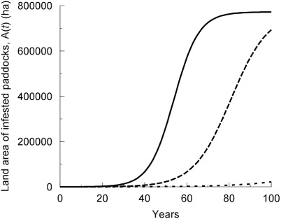
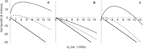
As a result of this uncertainty about an appropriate value for r, values twice (r = 0.1134) and three times (r = 0.1702) the default value of 0.0567 were considered. The resultant growth curves for the land area occupied are illustrated (for the case when A₀ = 80 ha) in Fig. 2. They result in a wide range of net benefit values for the containment programme (Fig. 3A). For example, the net benefit of –$173,178 predicted with A₀ = 80 ha and r = 0.0567 (solid line in Fig. 3A at A₀ = 80 ha), increases to a positive $822,836 with a doubling of the growth rate to r = 0.1134 (long-dashed line in Fig. 3A). For this assumption, the time required for the weed to spread to occupy 90% of its maximum habitable area halves from T₉₀ = 201 years, when r = 0.0567, to T₉₀ = 101 years when r = 0.1134. The containment programme, with this assumption, would be considered economically worthwhile. This value of r is similar to that calculated from data with the fringe classification excluded (r = 0.1297, Table 3) and may better represent the spread rate under the current climate. A trebling of r from its default value to r = 0.1702, which may better reflect growth rates under a changing climate, and hence over the next 100 years, increases the net benefit at A₀ = 80 ha to $5,246,318, further increasing the economic justification for the containment programme. This large influence of the assumed rate of spread on the net benefit of a containment programme for N. neesiana in Canterbury is also evident in the earlier analysis (Harris 2010). In that spatially implicit spread model, infestations grew in local plant density (according to a logistic model) and in land area occupied (local spread) giving rise annually to new infestations (long distance spread) at a land area occupied threshold of 560 ha. In the ‘Harris’ model, the net benefit of the containment programme increased substantially with the assumed annual rate at which the land area occupied by an infestation increased in size and also with the rate of increase in plant density within an infestation. It gave negative net benefits at low rates particularly when the costs associated with spread were assumed to be low (Harris 2010).

Figure 2 The logistic relationship, A(t), (Equation 1) for the growth in land area infested by N. neesiana in Canterbury for the case when A₀ = 80 ha and where: the growth rate r = 0.0567 (T₉₀ = 201 years) (- - -); r = 0.1134 (T₉₀ = 101 years) (-----); r = 0.1702 (T₉₀ = 67 years) (^_____).

Figure 3 Relationship between the net benefit of a containment programme for Nassella neesiana in Canterbury under a regional pest management plan and the size of the population to be contained (A₀ in the model) and its sensitivity to parameters r, f and i. In A: (^_____) r = 0.0567 (T₉₀ = 201 years); (- - -) r = 0.1135 (T₉₀ = 101); (-----) r = 0.1702 (T₉₀ = 67). In B: (^_____) f = 0.25; (- - -) f = 0.50; (-----) f = 0.75. In C: (^_____) i = 0.08; (- - -) i = 0.04 (-----) i = 0.03.

Our model's sensitivity to r reveals a need for reliable data from which the spread rate can be estimated for weeds being proposed as subjects for control programmes under regional pest management plans. Date-coded presence/absence records collected in structured statistically valid sampling programmes (Elzinga et al. 2001) could provide this data.

Also evident is that as A₀ increases in the model with all other parameters kept at their default values, the net benefit of the containment programme declines (solid line in Fig. 3A). This is because the present value of the cost of containment, TC_1, increases with the size of the containment area more rapidly than does the present value of the loss prevented by containment, TC₀. This is a result of the containment costs scaling directly with containment area and being incurred mainly in the first years when the discounting has little effect, while the losses prevented are greatest in the future but reduced by discounting. By contrast, when the rate of spread, r, is set greater than its default value, which may be justifiable as discussed above, then the net benefit shows a curved response to increase in A₀, revealing a ‘window’ in A₀ of positive net benefit that widens with increasing rate of spread (dashed lines in Fig. 3A). This phenomenon results from the value of the loss prevented by containment, TC₀, initially increasing relatively more rapidly than the cost of containment, TC₁, as A₀ increases. This in turn is a result of a shortened ‘lag phase’ in the spread as the starting point, A₀, increases (the growth curves [Fig. 2] shifting bodily to the left as A₀ increases) which means the losses prevented (benefits) begin to occur earlier, where discounting has relatively little effect compared with later years. But the direct scaling of the cost of containment as A₀ increases eventually begins to dominate and the net benefit (TC₀ – TC₁) then falls and becomes negative; this occurs at an infested area of A₀ = 5800 ha with the default value of r doubled to r = 0.1134 (Fig. 3A).

This analysis of the model's response to the size of the infested area in Canterbury where containment of N. neesiana is proposed, A₀, indicates that containment to an area ranging in size from 80 to 5800 ha would yield a positive net benefit under an assumed spread rate double that of the default value which, as discussed, may be reasonable. It seems probable that the actual containment area is well within this range, since additional infestations discovered in the locality of the 80 ha site where the weed was first discovered in 2008 amount to approximately 280 ha (Laurence Smith, pers. comm.).

Variation in parameters f and i

In contrast with r, the value assumed for the fractional loss in production due to N. neesiana, f, at the default value for r, has relatively little effect on the net benefit of containment at any value of A₀ (Fig. 3B).

The value assumed for the discount rate, i, does however have a substantial effect (Fig. 3C). When i = 0.08, i.e. the default value, the net benefit is negative for all values of A₀ at the default values of the other parameters (solid line in Fig. 3C). However, when i is halved to i = 0.04, the net benefit is positive up to A₀ = 1800 ha and when it is reduced further to i = 0.03, the net benefit increases substantially and remains positive up to A₀ = 13,000 ha (Fig. 3C). This sensitivity to i raises the issue of what its appropriate value should be. Prior to 2008, the social discount rate used in New Zealand was 0.10 (Parker 2011). In some European countries and parts of the USA, social discount rates of 0.03 to 0.04 are used for evaluating long-term projects of public benefit (Parker 2011). There is substantial supporting literature to suggest that social discount rates may often be set too high (Weitzman 1994; Caplin & Leahy 2000). Given that the invasion of N. neesiana on pastoral land in Canterbury would create a costly and essentially irreversible environmental problem for future generations of sheep and beef farmers, affecting both land values and the use to which the land could be put (not unlike climate change, for example), our default model discount rate of i = 0.08 may, arguably, be too high (Giera & Bell 2009).

Boundary conditions for NPV = 0

Although we have seen how sensitive (independently) the modelled net benefit of the proposed containment programme for N. neesiana is to spread rate r, and discount rate i, across a range of initial infestation size A₀, and how relatively insensitive it is to the fractional loss in production f, further insight can be gained by visualising the interacting effects of these parameters. To enable this we solved the net benefit equation (Equation 7) for net benefit = 0 for a wide range of parameter values. When this boundary condition is plotted as r (or T₉₀) versus i (Fig. 4), the parameter space to its left is where the net benefit >0. Here we can see, for example, in three illustrated cases where the size of the containment area is A₀ = 80 ha (Fig. 4A–C), how the r by i parameter space where net benefit >0, increases with the value of f, the assumed impact of the weed under a spread scenario. We can also see for the default case with production impact f = 0.25 (Fig. 4B), and also when doubled to f = 0.5 (Fig. 4C), how relatively small reductions in the discount rate and/or small increases in the assumed rate of spread rate from their default values (illustrated by the * in graphs) ‘push’ the model over the NPV = 0 boundary line into positive net benefit space. This is also the case when the containment area is A₀ = 800 ha, 10-fold greater than the default value (A₀ = 80 ha) (Fig. 4E– F). By contrast, if we assume that the weed has a much lower impact e.g. reducing production by only 2.5% (f = 0.025), then the containment programme would yield a positive net benefit only under assumptions of a greatly increased spread rate or a very low discount rate (Fig. 4A, D).

Figure 4 Relationships between the parameters r (spread rate, or T₉₀ [years to 90% saturation, Equation 2]) and i (discount rate) that satisfy the boundary condition that the net benefit (or NPV) is zero: A, A₀ = 80, f = 0.025; B, A₀ = 80, f = 0.25; C, A₀ = 80, f = 0.5; D, A₀ = 800, f = 0.025; E, A₀ = 800, f = 0.25; F, A₀ = 800, f = 0.5. In the parameter space to the left of these boundary lines, NPV > 0 and the containment programme would be economically worthwhile. The default model parameter values r = 0.0567 (T₉₀ = 201 years to 90% saturation) and i = 0.08 shown by *.

Concluding discussion

Based on the model presented here, using the default parameter values, the decision-maker could be justified in a decision not to proceed with the containment programme for N. neesiana in Canterbury. However, relatively small changes in the values of the weed's spread rate and the economic discount rate in the model result in a positive net benefit providing support for the programme. Given this uncertainty, it is tempting to call for additional studies to secure more precise estimates of the likely rate of future spread of the weed and to determine an appropriate discount rate. But deferring a response decision while these new data are being obtained would allow the weed to spread and result in a greater cost of containment and thus a lower net benefit estimate in a future calculation. It could also raise the cost of the modelling to a level unaffordable by the agency involved. Under these circumstances the decision-maker could give greater consideration to non-monetary impacts using tools such as multi-criteria decision analysis (Liu et al. 2011). For example, the animal welfare impacts of N. neesiana attributable to its penetrating seeds could be taken into account. Furthermore, the regional decision maker might also take account of the costs of spread at the national scale rather than only at the regional scale as in the analysis presented here. A national-scale analysis would result in a higher (and likely positive) net benefit since very large tracts of land throughout New Zealand are climatically suitable for N. neesiana (Bourdôt et al. 2010b).

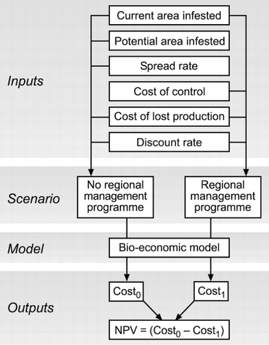
The method described here for evaluating the economics of a containment programme for N. neesiana in Canterbury would be equally suitable for evaluating containment programmes for other weed species and for the other types of programmes (exclusion, eradication, sustained control) as defined by the Biosecurity Act (Ministry for Primary Industries 2013). The method is summarised in the diagram in Fig. 5.

Figure 5 Diagrammatic representation of the method developed for conducting a cost-benefit analysis of a regional weed management programme proposed under a regional pest management plan.

Acknowledgements

This project was conducted as part of the Beating Weeds project led by Landcare Research with funding from the New Zealand Ministry of Business, Innovation and Employment. We thank Simon Harris, Harris Consulting Limited, Christchurch, New Zealand, for helpful advice on the structure of the model.

References

- Alan Herbarium 2014. CHR 632467 – Nassella neesiana (Trin. & Rupr.) Barkworth. Lincoln, Systematics Collection Data (SCD), Landcare Research. https://scd.landcareresearch.co.nz/Specimen/CHR%20632467?collection=CHR&search Collection=All&query=Nassella%20neesiana¤tDisplayTab=list&pageNumber=0&sortField=relevance (accessed 1 October 2014).
- AsureQuality 2009. AgriBaseTM. http://www.asurequality.com/capturing-information-technology-across-the-food-supply-chain/agribase-database-of-new-zealand-rural-properties.cfm (accessed 14 July 2015).
- Bell MD 2006. Spread of Chilean needle grass (Nassella neesiana) in Marlborough, New Zealand. New Zealand Plant Protection 59: 266–270.
- Bourdôt G, Fowler SV, Edwards GR, Kriticos DJ, Kean JM, Rahman A et al. 2007. Pastoral weeds in New Zealand: status and potential solutions. New Zealand Journal of Agricultural Research 50: 139–161.
- Bourdôt G, Harris S, Lamoureaux S 2010c. Integrating CLIMEX, land-use data and economic theory in weed risk analysis: Nassella neesiana in New Zealand as a case study. Proceedings of 4th Int. Pest Risk Modelling and Mapping Workshop—Pest risk in a Changing World. 15 p.
- Bourdôt GW, Hurrell GA 1989. Cover of Stipa neesiana Trin. and Rupr. (Chilean needle grass) on agricultural and pastoral land near Lake Grassmere, Marlborough. New Zealand Journal of Botany 27: 415–420.
- Bourdôt GW, Hurrell GA, Saville DJ 1998. Weed flora of cereal crops in Canterbury, New Zealand. New Zealand Journal of Crop and Horticultural Science 26: 233–247.
- Bourdôt GW, Lamoureaux SL, Kriticos DJ, Watt MS, Brown M 2010a. Current and potential distributions of Nassella neesiana (Chilean needle grass) in Australia and New Zealand. 17th Australasian Weeds Conference. Pp. 424–427.
- Bourdôt GW, Lamoureaux SL, Watt MS, Manning L, Kriticos DJ 2010b. The potential global distribution of the invasive weed Nassella neesiana under current and future climates. Biological Invasions 14: 1545–1556.
- Caplin A, Leahy J 2000. The social discount rate. Cambridge, MA, National Bureau of Economic Research. 29 p.
- Cousens R, Mortimer M 1995. Dynamics of weed populations. Cambridge, Cambridge University Press.
- Elzinga CL, Salzer DW, Willoughby JW, Gibbs JP 2001. Monitoring plant and animal populations. Tendoy, ID, Blackwell Science.
- Giera N, Bell B 2009. Economic costs of pests to New Zealand. MAF Biosecurity New Zealand Technical Paper no. 2009/31. Wellington, Biosecurity New Zealand, Ministry of Agriculture and Forestry.
- Harris S 2010. Meeting the requirements of the Biosecurity Act 1993: economic evaluation of regional pest management strategy for plant pests. Report (on Chilean needle grass) prepared for Environment Canterbury. Christchurch, Harris Consulting. 16 p.
- Liu S, Sheppard A, Kriticos DJ, Cook D 2011. Incorporating uncertainty and social values in managing invasive alien species: a deliberative multi-criteria evaluation approach. Biological Invasions. doi:10.1007/s10530-011-0045-4
- Lynn I, Manderson A, Page M, Harmsworth G, Eyles G, Douglas G et al. 2009. Land use capability survey handbook. 3rd edition. Hamilton, AgResearch Ltd, Landcare Research NZ Ltd, Institute of Geological and Nuclear Sciences Ltd.
- McLaren DA, Stajsic V, Gardener MR 1998. The distribution and impact of South/North American stipoid grasses (Poaceae: Stipeae) in Australia. Plant Protection Quarterly 13: 62–70.
- Meat & Livestock Australia and Australian Wool Innovation Limited 2014. Chilean needle grass case studies—four case studies of farmers managing Chilean needle grass in grazing systems. http://www.wool.com/globalassets/start/on-farm-research-and-development/production-systems-eco/pastures/weed-and-pest-management/chileanneedlegrass_casestudies_web1.pdf (accessed 8 August 2014).
- Ministry for Primary Industries 2013. Proposed national policy direction for pest management plans and programmes. MPI Discussion Paper no. 2013/14. Wellington, New Zealand Government. 39 p.
- Ministry for Primary Industries 2014. Biosecurity Act 1993. http://www.legislation.govt.nz/act/public/1993/0095/latest/DLM314623.html (accessed 10 September 2014).
- Ministry of Agriculture and Forestry 2009. Pastoral monitoring Canterbury/Marlborough Hill Country sheep and beef. Wellington, New Zealand Government.
- Ministry of Agriculture and Forestry 2012. Pastoral monitoring Canterbury/Marlborough Hill Country sheep and beef. Wellington, New Zealand Government.
- New Zealand Treasury 2005. Cost benefit analysis primer. Wellington, The Treasury. http://www.treasury.govt.nz/publications/guidance/planning/costbenefitanalysis/primer (accessed 1 October 2014).
- New Zealand Treasury 2008. Public sector discount rates for cost benefit analysis. Wellington, The Treasury. http://www.treasury.govt.nz/publications/guidance/costbenefitanalysis/discountrates (accessed 1 October 2014).
- New Zealand Treasury 2010. Cost benefit analysis including public sector discount rates. Wellington, The Treasury. http://www.treasury.govt.nz/publications/guidance/planning/costbenefitanalysis (accessed 18 September 2014).
- Parker C 2011. Economics like there's no tomorrow. Wellington, New Zealand Institute of Economic Research. 5 p.
- Snell K, Grech C, Jamie D 2007. National best practice management manual—Chilean needle grass. Melbourne, Victorian Government.
- Terralink 2009. Land cover database of New Zealand. http://www.terralink.co.nz/products_services/satellite/_cover_database_of_new_zealand/index.htm (accessed 15 February 2014).
- Weiss J, Morfe TA, McLaren D 2002. Assessing the financial implications of alternative investment options in weed control. In: Spafford Jacob H, Dodd J, Moore J eds. 13th Australian Weeds Conference Vol: 13. Perth, WA, Plant Protection Society of Western Australia Inc. for the Council of Australian Weed Science Societies. Pp. 505–508.
- Weitzman ML 1994. On the ‘environmental’ discount rate. Journal of Environmental Economics and Management 26: 200–209.