Does one size fit all? An evaluation of length–weight relationships for New Zealand's freshwater fish species

Abstract

Length–weight relationships are a fundamental tool for assessing populations and communities in fisheries science. Many researchers have collected length–weight data throughout New Zealand, yet parameters describing these relationships remain unpublished for many species of freshwater fish. We compiled 285,124 fish records from researchers and institutions across New Zealand to parameterise length–weight equations, using both power and quadratic models, for 53 freshwater species belonging to 13 families. The influence of location and sex on length–weight relationships was also assessed. Location, in particular, generated different length–weight relationships for 65% of the species examined. Length–weight equations were validated by comparing predicted weights against independently measured weights from 25 electrofished sites across New Zealand and the equations were highly accurate (R²>0.99). Recommendations are made about how to robustly apply this new resource which should assist freshwater fisheries researchers throughout New Zealand.

Keywords:

• length
• weight
• fish
• freshwater
• habitat type
• New Zealand

View correction statement:

Corrigendum

Introduction

Length–weight relationships (LWR) have been used to assess populations and communities in fisheries science since the beginning of the 20th century (Froese 2006). Understanding how fish weight changes as a function of length is fundamental information for fisheries scientists trying to deduce age structure (Jellyman 1997), calculate growth rates (Hansen & Closs 2009), model bioenergetics (Hayes et al. 2000; Booker et al. 2004) or quantify some other aspect of fish population dynamics (Safran 1992). LWR are required for: 1) estimating weight from fish lengths when time or technical constraints means they cannot be recorded in the field; 2) use in stock assessment models when converting growth in length to growth in weight (Bajer & Hayward 2006); 3) estimating biomass of a fish community using only length and species data (Greig et al. 2010); 4) estimating fish condition factor (Hiddink et al. 2011); and 5) making comparisons of fish life history characteristics (Fonseca & Cabral 2007). Despite this information being central to many aspects of fisheries ecology it was not considered ‘interesting science’ that warranted publication for many years during the latter 20th and early 21st centuries (Froese 2006). However, a special issue in 2006 (Length–weight-relationships in fish: new findings and concepts, Journal of Applied Ichthyology Volume 22, Issue 4) devoted to publishing LWR drew attention to the decline in the publication of these data and, since then, there has been a resurgence in papers in this area of fisheries science (e.g. Satrawaha & Pilasamorn 2009; Verreycken et al. 2011).

New Zealand's freshwater fish fauna now contains over 65 fish species (Allibone et al. 2010), and although basic biological data (e.g. length, weight) have been collected for many of these species, much of it remains unpublished. The objective of this paper was to produce LWR for as many freshwater fish species in New Zealand as possible. Whilst some New Zealand species have no published length–weight data, more common species may have multiple LWR published (e.g. longfin eel, Jellyman 1974; Todd 1980; Chisnall 1989; Chisnall & Hicks 1993; and more), so knowing which equation to apply to a particular dataset can be problematic. Moreover, LWR could vary with abiotic or sex-dependent factors so a secondary objective of the study was to evaluate if LWR differed between location or fish sex.

Methods

Dataset assembly

From March–July 2012, requests were sent out to researchers and institutions who we thought might have length–weight data on various New Zealand freshwater fish species. To accompany the data, information was requested regarding: 1) the region where it was collected; 2) whether the data was wet or dry weight; 3) the measuring method used (e.g. fork length, total length); and 4) whether the material had been preserved prior to measuring. In addition to this, a range of New Zealand fisheries publications were examined (e.g. papers, reports, theses) and data extracted if the above information could be ascertained. Some researchers and publications provided data on the sex of certain species, which was also used.

The vast majority of data contributed was wet-weight data but we also requested dry-weight data because this is useful for bioenergetic and food web studies, but is increasingly difficult to obtain permission to collect. The recorded precision across both datasets was relatively consistent for length and weight. Observations of the length of wet fish were generally recorded to the nearest 1 mm with the exception of fish less than 50 mm that were occasionally recorded to the nearest 0.5 mm and some large trout (>500 mm) that were recorded to the nearest 5 mm. Weighing precision varied from ± 0.001 g to ± 10 g depending on fish size (wet-weight range: 15–1565 mm). Methods for determining fish dry-weight varied slightly between researchers with temperatures for drying varying from 50–60 °C. Drying time was generally between 24–48 h with drying time increasing with fish size to ensure a comparable level of drying between small and large fish. All dried fish were measured to the nearest 1 mm and small fish (i.e. non-migratory galaxiids) were weighed to the nearest 0.1 mg and large fish (i.e. eels) were weighed to the nearest 0.1 g.

Controlling for bias in the data set

1. Gear. The type of gear used to capture fishes can introduce bias into LWR by selecting for particular fish sizes or body types (e.g. fyke nets capture large individuals and gill nets will select for fat fish over slimmer ones of the same length). However, we did not apply any weightings or corrections for gear type. Whilst some species recorded in our dataset are generally only caught using one gear type (e.g. non-migratory galaxiids with electrofishing), we did not consider gear bias a major problem because gear type/fishing technique often changes with fish size. For example, small eels and salmonids are generally sampled with electrofishing but larger individuals are usually caught with fyke nets or angling respectively, so the problem of gear bias is reduced because a variety of gear types are used to capture fish of different sizes.

2. Size range. LWR can be affected by the observed size range (Hiddink et al. 2011). Very small fish increase in length at a greater rate than they grow in other dimensions, so early life stages are often excluded if they do not resemble the adult body form (Safran 1992). Since larval/fry stages may not resemble the adult body form for some New Zealand fish species (e.g. torrentfish, McDowall 1994), we excluded all fish less than 15 mm.

3. Growth stanzas. Previous studies of LWR have sometimes found multiple growth stanzas within a species such that the slope of the LWR is significantly different when they are small compared to when they are larger (e.g. Fulton 1904). Different growth stanzas have been found to be correlated with reproductive age and ontogenetic dietary shifts (Stergiou & Fourtouni 1991), and not recognising these inflection points in LWR can result in slope values being under or overestimated (Froese 2006). Whilst we attempted to report data over as wide a range of fish lengths as possible, if a growth stanza was identified from a visual inspection of a species’ log-log plot, then data for small fishes was omitted.

4. Partial size spectrum. Large numbers of observations are not required to calculate a LWR and as few as 10 small, 10 medium and 10 large fish will normally produce a reliable relationship (Froese 2006). Of greater importance than the number of individuals is the size range that is encompassed by the data because misleading slope and intercept values can result if only a partial size spectrum is used. The LWR we present should only be considered accurate for the range of fish sizes we report on, especially if an equation is calculated using only a partial size spectrum (e.g. adult fish only).

5. Differences between sexes. Males and females can have different LWR but accurately determining a fish's gender may only be possible upon internal inspection once it has been killed (e.g. non-migratory galaxiids) unless a species has obvious colouration differences (e.g. redfin bully) or physical differences (e.g. adult brown trout). Fish researchers usually try to return fish unharmed, and thus often unsexed, so we did not request data on fish sex. However, for species where sufficient data on fish sex were supplied, significant gender differences were tested for.

6. Seasonal differences. LWR may show some seasonal variation since food availability, level of gonad development, etc. is not constant throughout the year. We could not control for seasonal sampling variation in our analysis because we did not request information on sampling season. We would speculate that there is likely to be a seasonal sampling bias in this dataset, favouring sampling during warmer months over colder months, but cannot know definitely. Consequently, our LWR may overestimate fish weights when being applied to samples from winter months.

Analysis of length–weight data

The dataset underwent five sequential steps for quality control; the first three are comparable to the method used by Verreycken et al. (2011). Firstly, length data were compared against the maximum length for each species as reported by McDowall (2000) or in FishBase (Froese & Pauly 2012). Any record where a fish was 25% larger than the maximum length for that species was considered erroneous and deleted (this criteria was not applied to non-migratory galaxiids as previously published maximum lengths were not considered reliable given the amount of new data available, instead a 180 mm maximum length was applied to these species). Secondly, any length records of fish less than 15 mm were removed (see previous section for rationale). The third step was to plot the LWR for each species and remove individuals with a weight that was more than double or less than half the expected weight (based on the fitted LWR); these were considered to be data-entry errors. Fourth, records were not used if fish had been frozen or chemically preserved (e.g. formalin, ethanol) prior to measuring because these preservation techniques can alter fish weight and length (Paradis et al. 2007). The one exception was Stokell's smelt where formalin-preserved fish were included because these were the only data available for that species. The final step was to remove all fish that were only identified to genus level (taxonomically indeterminate taxa listed in Allibone et al. 2010 were included where data were available).

Following quality control we selected a method for constructing our LWR. There are two main techniques used to calculate length–weight equations and these involve either pooling all data on individuals to calculate a species equation (e.g. Verreycken et al. 2011) or calculating equations for different populations and then combining these to produce a species equation (e.g. Cooney & Kwak 2010). We selected the pooled data method because we had not requested that data contributors separate their data at the population level (e.g. between sites).

LWR on pooled data were produced for each species by regressing log₁₀W against log₁₀L. The significance of each LWR was assessed using a linear model in the R statistical package (R Development Core Team 2012). For simplicity, the fitted model for each species was in the form of a power function using the equation:

(1)

where W is whole body weight in grams, L is length in mm, a is the intercept value and b the slope value. The relationship between a and b values was also assessed because these values are interdependent and variation in a is strongly linked to fish body shape (Froese 2006). For example, two species may have similar values for b but have much different values for a because one species has a ‘fusiform’ body shape whilst the other has an ‘eel-like’ body form. In our dataset, fish from the families Anguillidae and Geotriidae were classified as ‘eel-like’, Pleuronectidae had ‘compressed’ body shape, Cyprinidae and Poeciliidae were ‘short and deep’ and the remaining families were considered to have ‘fusiform’ shape. The influence of fish body shape on a and b values was assessed using a homogeneity of slopes test. If a non-significant interaction term was returned, then analysis of covariance (ANCOVA) was conducted.

The power function of Equation 1 is commonly used in fisheries research to describe the relationship between length and weight, but different forms of this empirical equation may better fit such data. Equations that include a quadratic term are becoming more common in analyses of length–weight data to account for curvature in log-log space. Including a quadratic term to predict LWR may improve the accuracy of estimated weights (e.g. Cooney & Kwak 2010), especially for species that can grow to a very large size. The equation that included a quadratic term was:

(2)

where W is whole body weight in grams, L is length in mm, a and b are analogous to the parameters from Equation 1 and c is the quadratic term that accounts for curvature in log-log space.

Standard forwards and backwards stepwise linear regression was used to identify which model was more adequate, a power or quadratic model. The Akaike information criterion (AIC; Akaike 1973) was used to apply a penalised log-likelihood method to evaluate the trade-off between degrees of freedom and fit of the model as the predictors were added or removed (Crawley 2002). Because selecting model terms on the basis of AIC alone has been shown to be liberal, a value of k=4 was used for the multiple of the number of degrees of freedom used to define the penalty for inclusion of a predictor in the stepwise procedure (Venables & Ripley 2002). This had the effect of retaining model terms for which the P value was less than 0.05.

Location and fish sex analyses

For fish species, ANCOVA was used to evaluate whether location (data was simplified from region to North/South Island) and fish sex (male/female) resulted in different LWR. Prior to the analyses, each dataset had observations removed so that equivalent size ranges were compared for each species in the ANCOVA. This data reduction was done because in initial analyses, significant differences were strongly influenced by data ranges rather than the covariate (i.e. the chance of detecting a significant difference was being inflated by having datasets that were calculating slopes and intercepts across contrasting fish size ranges). For consistency, power equations were used across these analyses to calculate the LWR. For each analysis, a minimum of 10 individuals had to be present for each level of the covariate (e.g. 10 male and 10 female fish of a species in the gender analysis). Due to data constraints, only wet-weight data was used in these analyses.

Evaluating the accuracy of the length–weight equations

Electrofishing data from across New Zealand were used to evaluate the accuracy of the length–weight equations produced from our analysis. We used electrofishing data from 25 sites to assess how accurately total fish weight at a site was predicted by the equations from Table 1 compared to the physically measured fish weight data. The data used for the comparison was independent as it had not been used to produce the length–weight equations. In this comparison the accuracy of both the power and quadratic equations were compared against total measured fish weight at each site.

Table 1 Estimated parameters of length–weight relationships for 53 freshwater fish species in New Zealand using wet-weight data (except for Stokellia anisodon which were preserved in formalin). Parameters are given for power equations and 95% CI for a are provided in Table S1. Quadratic parameters are supplied in Table S2 if they were selected as the better model. For the ‘Origin’ column: N = native, I = introduced, M = marine wanderer, E = extinct. NA = not available.

Family Species name (Naming authority)	Common name	Origin	n	Length measure (TL/FL)	Length range (mm)	Weight range (g)	R^2	a	b	95% CI b
Anguillidae
Anguilla australis (Richardson 1841)	Shortfin eel	N	34891	TL	72–1310	0.3–3955	0.975	4.906×10^−7	3.224	3.218–3.229
Anguilla dieffenbachii (Gray 1842)	Longfin eel	N	41070	TL	88–1565	0.7–15000	0.975	3.624×10^−7	3.307	3.301–3.312
Anguilla reinhardtii (Steindachner 1867)	Spotted eel	N	27	TL	408–760	177–1513	0.935	2.975×10^−7	3.360	2.996–3.725
Cyprinidae
Carassius auratus (Linnaeus 1758)	Goldfish	I	3986	FL	15–396	0.05–2435	0.980	1.253×10^−5	3.125	3.111–3.138
Ctenopharyngodon idella (Valenciennes 1844)	Grass carp	I	398	FL	140–604	39.6–3870	0.967	1.086×10^−5	3.049	2.994–3.104
Cyprinus carpio (Linnaeus 1758)	Koi carp	I	2615	FL	45–700	2–8373	0.985	1.694×10^−5	3.048	3.034–3.062
Hypophthalmichthys molitrix (Valenciennes 1844)	Silver carp	I					–	–	–
Leuciscus idus (Linnaeus 1758)	Orfe	I					–	–	–
Scardinius erythrophthalmus (Linnaeus 1758)	Rudd	I	1548	FL	67–340	4–813	0.975	7.525×10^−6	3.168	3.142–3.193
Tinca tinca (Linnaeus 1758)	Tench	I	363	FL	37–510	0.7–1804	0.991	1.797×10^−5	2.983	2.953–3.012
Eleotridae
Gobiomorphus alpinus (Stokell 1962)	Tarndale bully	N					–	–	–
Gobiomorphus basalis (Gray 1842)	Cran's bully	N	17	TL	40–107	0.8–16	0.724	1.027×10^−4	2.494	1.646–3.341
Gobiomorphus breviceps (Stokell 1940)	Upland bully	N	3323	TL	22–131	0.1–30	0.945	1.127×10^−5	3.025	2.999–3.049
Gobiomorphus cotidianus (McDowall 1970)	Common bully	N	1799	TL	16–140	0.03–30	0.983	6.160×10^−6	3.152	3.133–3.171
Gobiomorphus gobioides (Valenciennes 1844)	Giant bully	N	363	TL	86–222	5–180	0.916	6.893×10^−6	3.145	3.046–3.244
Gobiomorphus hubbsi (Stokell 1959)	Bluegill bully	N	625	TL	31–92	0.1–6.5	0.951	1.798×10^−6	3.393	3.332–3.453
Gobiomorphus huttoni (Ogilby 1894)	Redfin bully	N	243	TL	38–111	0.4–17	0.945	2.574×10^−6	3.329	3.227–3.431
Galaxiidae
Galaxias anomalus (Stokell 1959)	Roundhead galaxias	N	5299	TL	36–106	0.2–8.8	0.931	2.345×10^−6	3.269	3.245–3.292
Galaxias argenteus (Gmelin 1789)	Giant kōkopu	N	298	TL	67–340	4.9–644	0.984	7.004×10^−6	3.121	3.075–3.166
Galaxias brevipinnis (Günther 1866)	Kōaro	N	573	TL	37–230	0.3–110	0.966	1.838×10^−6	3.324	3.272–3.375
Galaxias cobitinis (McDowall/Waters 2002)	Lowland longjaw galaxias	N	7455	TL	19–82	0.05–2.9	0.813	4.490×10^−6	3.039	3.006–3.072
Galaxias depressiceps (McDowall/Wallis 1996)	Flathead galaxias	N	1692	TL	26–116	0.1–11	0.962	1.821×10^−6	3.342	3.310–3.373
Galaxias divergens (Stokell 1959)	Dwarf galaxias	N	4772	TL	20–90	0.05–6.3	0.922	6.252×10^−6	3.003	2.978–3.028
Galaxias eldoni (McDowall 1997)	Eldon's galaxias	N	4577	TL	18–156	0.06–37	0.975	3.636×10^−6	3.186	3.171–3.200
Galaxias fasciatus (Gray 1842)	Banded kōkopu	N	1269	TL	38–248	0.2–228	0.982	1.205×10^−6	3.438	3.412–3.464
Galaxias gollumoides (McDowall/Chadderton 1999)	Gollum galaxias	N	6	TL	65–92	2.7–7.3	0.739	1.341×10^−5	2.914	0.510–5.317
Galaxias gracilis (McDowall 1967)	Dwarf inanga	N					–	–	–
Galaxias macronasus (McDowall/Waters 2003)	Bignose galaxias	N	2357	TL	21–110	0.1–9.6	0.833	7.675×10^−6	2.896	2.844–2.949
Galaxias maculatus (Jenyns 1842)	Īnanga	N	1730	TL	36–140	0.2–18	0.962	4.990×10^−7	3.566	3.533–3.599
Galaxias paucispondylus (Stokell 1938)	Alpine galaxias	N	1105	TL	33–120	0.1–9.7	0.897	7.856×10^−6	2.904	2.846–2.962
Galaxias postvectis (Clarke 1899)	Shortjaw kōkopu	N	588	TL	50–243	0.9–204	0.984	2.114×10^−6	3.333	3.299–3.368
Galaxias prognathus (Stokell 1940)	Upland longjaw galaxias	N	386	TL	38–86	0.2–3.4	0.848	3.642×10^−6	3.061	2.932–3.191
Galaxias pullus (McDowall 1997)	Dusky galaxias	N	2765	TL	26–158	0.1–40	0.978	2.307×10^−6	3.295	3.276–3.314
Galaxias ‘sp. D.’	Clutha flathead galaxias	N	1940	TL	26–136	0.1–26	0.972	2.848×10^−6	3.226	3.201–3.250
Galaxias ‘Northern sp.’	Northern flathead galaxias	N					–	–	–
Galaxias ‘Southern sp.’	Southern flathead galaxias	N	20	TL	70–106	3.1–9.7	0.956	1.111×10^−5	2.947	2.634–3.259
Galaxias ‘Teviot’	Teviot flathead galaxias	N					–	–	–
Galaxias vulgaris (Stokell 1949)	Canterbury galaxias	N	1945	TL	28–171	0.1–38	0.957	3.338×10^−6	3.196	3.166–3.226
Neochanna apoda (Günther 1867)	Brown mudfish	N	660	TL	29–162	0.1–23	0.973	4.694×10^−6	3.025	2.986–3.063
Neochanna burrowsius (Phillipps 1926)	Canterbury mudfish	N	1296	TL	30–148	0.1–22	0.938	6.199×10^−6	2.986	2.945–3.028
Neochanna diversus (Stokell 1949)	Black mudfish	N	555	TL	32–157	0.2–24	0.981	5.483×10^−6	3.017	2.982–3.052
Neochanna heleios (Ling/Gleeson 2001)	Northland mudfish	N
Neochanna rekohua (Mitchell 1995)	Chatham mudfish	N
Geotriidae
Geotria australis (Gray 1851)	Lamprey	N	264	TL	23–614	0.1–173	0.972	2.030×10^−5	2.479	2.427–2.530
Ictaluridae
Ameiurus nebulosus (Lesueur 1819)	Brown bullhead catfish	I	5767	FL	42–420	0.8–1129	0.979	5.981×10^−6	3.137	3.125–3.149
Mugilidae
Aldrichetta forsteri (Valenciennes 1836)	Yelloweye mullet	M	28	FL	198–390	107–680	0.980	2.111×10^−5	2.902	2.773–3.070
Mugil cephalus (Linnaeus 1758)	Grey mullet	M	146	FL	138–520	33–2054	0.975	8.632×10^−6	3.078	2.997–3.159
Percidae
Perca fluviatilis (Linnaeus 1758)	Perch	I	3218	FL	23–441	0.1–1614	0.978	1.543×10^−5	2.984	2.968–2.999
Pinguipedidae
Cheimarrichthys fosteri (Haast 1874)	Torrentfish	N	711	FL	31–140	0.4–40	0.977	1.3929×10^−5	2.974	2.940–3.008
Pleuronectidae
Rhombosolea leporina (Günther 1862)	Yellowbelly flounder	M	526	TL	46–369	1.1–721	0.983	1.490×10^−5	2.989	2.955–3.022
Rhombosolea plebeia (Richardson 1843)	Sand flounder	M	503	TL	46–328	1.1–599	0.962	8.476×10^−6	3.117	3.063–3.172
Rhombosolea retiaria (Hutton 1874)	Black flounder	N	355	TL	75–391	5.7–1003	0.944	6.154×10^−5	2.765	2.694–2.836
Poeciliidae
Gambusia affinis (Baird/Girard 1853)	Mosquito fish	I	188	TL	15–51	0.02–2.0	0.906	1.018×10^−6	3.681	3.512–3.860
Poecilia latipinna (Lesueur 1821)	Sailfin molly	I					–	–	–
Poecilia reticulata (Peters 1859)	Guppy	I					–	–	–
Ptereleotridae
Parioglossus marginalis (Rennins/Hoese 1985)	Dart goby	I					–	–	–
Retropinnidae
Prototroctes oxyrhynchus (Günther 1870)	Grayling	E					–	–	–
Retropinna retropinna (Richardson 1848)	Common smelt	N	33270	FL	20–125	0.01–22	0.930	3.612×10^−6	3.105	3.097–3.115
Stokellia anisodon (Stokell 1941)	Stokell's smelt	N	50	FL	70–81	N/A	0.683	2.778×10^−5	2.650	N/A
Salmonidae
Oncorhynchus mykiss (Walbaum 1792)	Rainbow trout	I	84262	FL	38–790	0.5–5550	0.939	2.101×10^−5	2.909	2.904–2.914
Oncorhynchus nerka (Walbaum 1792)	Sockeye salmon	I	47	FL	197–465	88–1336	0.994	2.357×10^−6	3.290	3.212–3.368
Oncorhynchus tshawytscha (Walbaum 1792)	Chinook salmon	I	3640	FL	30–1070	0.1–21110	0.990	6.401×10^−6	3.099	3.089–3.109
Salmo salar (Linnaeus 1758)	Atlantic salmon	I	40	FL	445–724	1134–2948	0.833	5.419×10^−3	1.994	1.701–2.288
Salmo trutta (Linnaeus 1758)	Brown trout	I	17662	FL	22–930	0.1–8172	0.995	1.332×10^−5	2.978	2.975–2.981
Salvelinus fontinalis (Mitchill 1814)	Brook char	I	518	FL	29–235	0.2–147	0.986	9.593×10^−6	3.007	2.975–3.038
Salvelinus namaycush (Walbaum 1792)	Mackinaw trout	I					–	–	–

Results

Of the 66 species we considered to be partly or wholly freshwater fish in New Zealand, we were able to produce LWR for 53 species belonging to 13 families (Table 1). For the most speciose family, Galaxiidae, LWR were calculated for 21 of the 26 species. Six LWR were calculated for Eleotridae and Salmonidae and five for Cyprinidae. LWR were calculated for all species belonging to the families Anguillidae, Geotriidae, Ictaluridae, Mugilidae, Percidae, Pinguipedidae and Pleuronectidae. Although no data were available for 13 species, these are relatively rare in New Zealand freshwaters.

The total length–weight dataset contained 285,124 fish records with 283,751 wet weights, 1,323 dry weights and 50 formalin-preserved fish (Tables 1, 2). We removed < 1% of all records from the dataset, which was much fewer than recent studies by Satrawaha and Pilasamorn (2009) and Verreycken et al. (2011) who discarded 19% and 3% of all records, respectively. Five species had over 10,000 records. These species were brown and rainbow trout, longfin and shortfin eel, and common smelt. New Zealand's four most-threatened fish species (Canterbury mudfish, lowland longjaw galaxias, Eldon's galaxias and Dusky galaxias; see Allibone et al. 2010) all had more than 1000 records available.

Table 2 Estimated parameters of length–weight power relationships for New Zealand freshwater fish species for which dry-weight data was available. Quadratic parameters are supplied in Table S3 if they were selected as the better model.

			Length	Length			95%		95%
			measure	range			CI		CI
FamilySpecies name	Common name	n	(TL/FL)	(mm)	R^2	a	a	b	b
Anguillidae
Anguilla australis	Shortfin eel	86	TL	54–385	0.983	2.999×10^−8	1.799×10^−8–4.998×10^−8	3.481	3.382–3.581
Anguilla dieffenbachii	Longfin eel	108	TL	66–647	0.978	1.390×10^−8	7.790×10^−9–2.479×10^−8	3.641	3.535–3.746
Eleotridae
Gobiomorphus breviceps	Upland bully	271	TL	24–94	0.968	2.155×10^−7	1.561×10^−7–2.973×10^−7	3.616	3.537–3.695
Gobiomorphus cotidianus	Common bully	76	TL	14–111	0.982	7.746×10^−7	5.061×10^−7–1.186×10^−6	3.297	3.193–3.402
Gobiomorphus gobioides	Giant bully	3	TL	52–81	0.998	1.227×10^−7	1.150×10^−11–1.309×10^−3	3.712	1.502–5.922
Gobiomorphus hubbsi	Bluegill bully	53	TL	48–76	0.787	1.498×10^−6	2.389×10^−7–9.389×10^−6	3.078	2.629–3.528
Galaxiidae
Galaxias brevipinnis	Kōaro	29	TL	35–105	0.978	1.400×10^−8	4.978×10^−9–2.479×10^−8	4.082	3.839–4.324
Galaxias maculatus	Īnanga	35	TL	42–101	0.917	1.229×10^−7	2.734×10^−8–5.520×10^−7	3.473	3.104–3.843
Galaxias paucispondylus	Alpine galaxias	67	TL	52–95	0.856	1.107×10^−6	2.993×10^−7–4.095×10^−6	3.068	2.757–3.380
Galaxias vulgaris	Canterbury galaxias	217	TL	60–137	0.936	3.831×10^−7	2.240×10^−7–6.550×10^−7	3.417	3.297–3.537
Pinguipedidae
Cheimarrichthys fosteri	Torrentfish	64	FL	49–136	0.984	4.261×10^−7	2.581×10^−7–7.033×10^−7	3.467	3.353–3.580
Salmonidae
Oncorhynchus mykiss	Rainbow trout	25	FL	61–185	0.984	3.472×10^−7	1.503×10^−7–8.020×10^−7	3.407	3.218–3.596
Oncorhynchus tshawytscha	Chinook salmon	68	FL	67–115	0.903	1.092×10^−7	2.906×10^−8–4.102×10^−7	3.735	3.434–4.036
Salmo trutta	Brown trout	221	FL	58–199	0.956	2.294×10^−6	1.560×10^−6–3.373×10^−6	3.050	2.963–3.137

Across the dataset, the coefficient of determination (i.e. R²) for all models ranged from 0.68–0.99 for wet-weight data and 0.79–0.99 for dry-weight data (Tables 1, 2). For all species, R² values less than 0.8 were associated with either low numbers of individuals or a limited size range. All fish families had mean R² values greater than 0.9 (when formalin-preserved smelt were excluded). However, there was a group of fishes whose weight was consistently the least predictable: the pencil galaxiids (G. cobitinis, G. divergens, G. macronasus, G. paucispondylus, G. prognathus). Despite having more than 16,000 records for these five species, the average R² value across the group was 0.86.

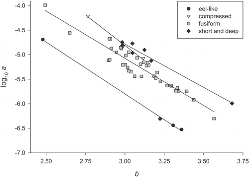
For the power equations, slope values for b varied in the wet-weight dataset from 1.99–3.68 (mean: 3.07±0.04) and from 3.05–4.08 (mean: 3.47±0.08) in the dry-weight dataset (Tables 1, 2). The slope value of 1.99 for Atlantic salmon was well outside the typical range of b values (2.5–3.5; Ricker 1975) because it was calculated using only adult fish. Values of b and log a were strongly related and the relationship between these parameters varied significantly with fish body shape (F_3,47=61.6, P< 0.001; Fig. 1). Moreover, a model with b and body shape as a categorical factor explained 94% of the variation in log a. All body shape regression lines had R² values greater than 0.9 and had intercept values that were significantly different from each other except for the ‘compressed’ and ‘short and deep’ categories. The ‘eel-like’ regression line showed the most departure from the other three (Fig. 1).

Figure 1 Scatterplot of log₁₀a and b parameters based on body shape for 52 New Zealand freshwater fish species. For clarity, the data point for Atlantic salmon has been omitted from the plot.

Within families containing multiple species, some taxa were always heavier across the size range analysed. For example, longfin eels were always heavier than shortfin eels of the same length, although spotted eels were actually heavier than either species across the limited size range for which data was available (Table 1). Giant kōkopu and giant bullies were both heavier than other similarly-sized galaxiid or bully species, respectively. For salmonids, rainbow trout was generally the heaviest species below 515 mm but beyond this length, Chinook salmon was heavier. Goldfish was the heaviest species within the family Cyprinidae although it only grows to around 400 mm in New Zealand (Table 1; McDowall 2000). Tench, grass carp and koi carp all grow longer than 400 mm, but koi carp is much heavier at these lengths (e.g. koi carp are more than 500 g heavier at 450 mm).

AIC and P-values indicated that quadratic models were more adequate than power models for 37 of the 52 species where wet-weight data was available and nine of the 14 species that also had dry-weight data. The inclusion of an extra model parameter meant that all quadratic models had higher R² values than power models. A comparison between power and quadratic equations showed that predicted fish weights were relatively similar across most of a species size range; therefore, only power equations were produced for Tables 3 and 4. However, when a species grew to be large, power equations predicted fish were heavier at their maximum size for 23 of the 37 species (62%). For example, at 700 mm the predicted weights of longfin and shortfin eels varied by 1% between power and quadratic equations, but at 1200 mm, power equations were predicting longfin eels to be 403 g heavier and shortfin eels to be 366 g heavier when compared to the predicted weights from quadratic equations.

Table 3 Differences in length–weight relationships between locations. Equations are only provided for those species where a significant difference between the North and South Islands was detected (the list of species for which no significant differences were detected are in Table S4).

Family
Species name	Common name	Island	n	a	b
Anguillidae
Anguilla australis	Shortfin eel	North	21723	3.9129×10^−7	3.2552
		South	13168	6.1403×10^−7	3.1952
Cyprinidae
Scardinius erythrophthalmus	Rudd	North	1134	7.6776×10^−6	3.1587
		South	414	4.6029×10^−6	3.2792
Eleotridae
Gobiomorphus cotidianus	Common bully	North	1375	6.6481×10^−6	3.1377
		South	423	2.0647×10^−6	3.4027
Galaxiidae
Galaxias argenteus	Giant kōkopu	North	86	1.3902×10^−5	2.9946
		South	212	5.9995×10^−6	3.1485
Galaxias divergens	Dwarf galaxias	North	2691	3.8140×10^−6	3.1286
		South	2081	2.6898×10^−5	2.6320
Galaxias fasciatus	Banded kōkopu	North	513	2.1307×10^−6	3.3208
		South	756	9.6888×10^−7	3.4865
Galaxias maculatus	Īnanga	North	1339	5.8634×10^−7	3.5282
		South	391	1.9799×10^−7	3.7754
Percidae
Perca fluviatilis	Perch	North	3107	1.7488×10^−5	2.9604
		South	111	4.1487×10^−6	3.2190
Pinguipedidae
Cheimarrichthys fosteri	Torrentfish	North	41	5.0381×10^−6	3.2052
		South	670	1.4706×10^−5	2.9616
Salmonidae
Oncorhynchus mykiss	Rainbow trout	North	83180	6.2808×10^−5	2.7335
		South	1082	1.0038×10^−5	3.0225
Salmo trutta	Brown trout	North	10656	1.5335×10^−5	2.9582
		South	7006	1.5114×10^−5	2.9492

Table 4 Differences in length–weight relationships for male and female fishes. Equations are only provided for those species where a significant difference between the sexes was detected. Note that values for a and b may be markedly different to those in Table 1 because less data was used across a more limited size range.

FamilySpecies name	Common name	P value	Sex	n	Range (mm)	a	b	95% CI b
Cyprinidae
Carassius auratus	Goldfish	0.02	Female	144	87–241	6.3760×10^−6	3.252	3.184–3.319
			Male	145	83–239	1.1234×10^−5	3.134	3.072–3.205
Cyprinus carpio	Koi carp	0.005	Female	265	243–633	9.8060×10^−6	3.147	3.029–3.265
			Male	510	231–630	2.6727×10^−5	2.970	2.905–3.035
Galaxiidae
Galaxias brevipinnis	Kōaro	0.01	Female	58	96–192	1.9255×10^−5	2.867	2.721–3.014
			Male	40	96–195	4.4570×10^−6	3.170	2.965–3.375
Percidae
Perca fluviatilis	Perch	0.04	Female	290	117–305	1.0284×10^−5	3.043	2.968–3.118
			Male	118	114–305	5.0490×10^−6	3.186	3.067–3.306
Salmonidae
Salmo trutta	Brown trout	<0.001	Female	846	177–600	5.4749×10^−5	2.742	2.704–2.781
			Male	747	170–605	1.2074×10^−4	2.604	2.558–2.650

Differences between locations

Of the 17 species for which there were sufficient records to compare LWR between the North and South Islands, significantly different LWR were found for 11 species (Table 3). Whilst shortfin eels were always heavier in the South Island and brown trout always heavier in the North Island, seven of the 11 species were initially heavier in North Island habitats but, as they grew, individuals in South Island habitats became heavier for a given size. For example, a 100 mm giant kōkopu would be 1.7 g heavier in the North Island, but if it grew to 300 mm a South Island fish would be 14 g heavier at that length. Similarly, a 100 mm perch would be 3.2 g heavier in the North Island, but a 300 mm perch would be 14 g heavier in the South Island. Both dwarf galaxias and torrentfish showed the reverse of this pattern as fish were initially heavier in the South Island but, as they grew, North Island fish became heavier than similarly-sized South Island fish.

Fish sex differences

The LWR of male and female fish were compared for 13 species. Significant fish sex differences were detected for the LWR of five species: goldfish; koi carp; kōaro; perch; and brown trout (Table 4), although three were only marginally significant (P<0.05). At their maximum size evaluated (see Table 4 for size range analysed), female goldfish, koi carp and brown trout were heavier than similar-sized males, whereas male kōaro and perch were heavier than females of the same length. Whilst different LWR are likely to occur in species where one sex can grow much larger than the other (e.g. female longfin eels grow much larger than males, McDowall 2000), our analysis would not detect a significant species difference since the size range that was evaluated was kept consistent for both sexes.

Evaluating the accuracy of the length–weight equations

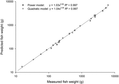
Total fish weight for the 25 electrofished sites varied across three orders of magnitude from 15.5–6259 g. When applying both the power and quadratic length–weight equations to the length data, very similar weight estimates were predicted by both equation types (Fig. 2). The power equations predicted a fish weight range from 17.4–7069 g and the quadratic equations predicted a range from 17.5–6945 g. Across the 25 sites, the mean difference between measured and predicted weights were 0.6±1.5% (range: −14.8–12.9%) for the power equations and 0.8±1.7% (range:−17.6–13.2%) for quadratic equations. Importantly, at sites where predicted weight estimates deviated by more than 10% from the measured weight, both power and quadratic equations were still predicting similar weights (i.e. within 3.5% of each other). Concurrence between both equation types suggests that the weights of the fishes at these sites were varying from what is commonly observed nationally, rather than the equations themselves being a poor predictor of total fish weight.

Figure 2 The relationship between measured and predicted fish weight for 25 sites around New Zealand. Predicted fish weights were calculated using both power and quadratic equations from Table 1. Note that two separate regression lines are not visible because the fitted relationships were equivalent when both methods were used.

Discussion

This paper has reported length–weight equations for 53 fish species found in New Zealand freshwaters. These equations should be both widely applicable and robust since the data have been assembled from across New Zealand and have used more than 500 fish in two-thirds of the wet-weight equations for individual species. When the equations were applied to an electrofishing dataset from five New Zealand regions, both the power and quadratic models performed well with the predicted site weights closely matching the measured site weights. Whilst the power and quadratic models produced very similar predicted weights, the quadratic equations (as supplied in Table 1) were statistically better models that better fitted the data. In other studies where both power and quadratic models have been fitted to species length–weight data, use of quadratic equations has been recommended (e.g. Cooney & Kwak 2010). Although the variation in predicted weights between the two equation types was negligible across the majority of a species’ size range, we would also recommend using the quadratic equations when supplied because power models had a slight tendency to overestimate the weight of very large individuals.

The goodness-of-fit for both equation types could have been improved by imposing stricter quality control criteria on the dataset. For example, Ogle and Winfield (2009) rejected datasets with an R² value less than 0.9. However, there is a trade-off between stricter quality control and discarding ‘real’ variation so the application of threshold values, such as an R² of 0.9, needs to be appropriate for the dataset being analysed. Applying Ogle and Winfield's (2009) threshold value in our dataset would have resulted in a large proportion of the pencil galaxiid data being discarded, but we would contend that such data should not be omitted because it indicates how variable the LWR can be for a species (or group of species). Moreover, pencil galaxiids often inhabit physically disturbed habitats and LWR with R² values less than 0.9 are likely to reflect variability in fish condition due to environmental harshness rather than the inclusion of outliers or different growth stanzas.

The influence of body form on length–weight relationships

Body shape is an important factor influencing the relationship between b and log a because fish species with the same body shape situate themselves along a body-shape-specific regression line (Froese 2006). The various body shapes (e.g. eel-like) have different intercept values for their respective regression line, but the lines are effectively parallel for each body shape. These parallel regression lines can provide researchers with a very useful tool for species that have no length–weight data available. For example, if weight data was required for an unidentified pencil galaxias, then Table 1 could be used to calculate a mean b value for the five pencil galaxias species (i.e. 2.98, range: 2.90–3.06). This b value of 2.98 and the knowledge that these fishes have a fusiform body shape would indicate that a log a of −5 should be used as the intercept value for an equation to calculate the weight of the unidentified fish species.

The influence of location and fish sex on length–weight relationships

The New Zealand fish fauna is strongly shaped by geographic gradients, such as latitude and altitude, because they produce different habitat conditions (e.g. thermal regimes) for fish to occupy (McDowall 2008; McDowall 2010). Therefore, we used the North and South Island to assess whether differences in location resulted in changes to the LWR for species that inhabit both islands. Only 17 species were available for a geographic comparison because for a species to be on both islands it generally needed to be either migratory or human-introduced; the exceptions were the non-migratory dwarf galaxias and upland bully that are present on both islands due to historic geographic processes (McDowall 2010). For seven of the 11 species with different LWR in the North and South Island, fish were initially heavier in the North Island when small but, as they grew to be large, South Island fish of equivalent size became heavier. There are many possible explanations for why this difference between LWR in the North and South Island occurs, such as temperature, fish physiology, growth rate, fish density, competition with introduced fish, etc. It is a finding that ‘asks more questions than it answers’ but one that should be of interest to fisheries and conservation managers because a positive correlation between fish weight and fecundity (Bagenal 1957; Quinn & Bloomberg 1992) could mean that large South Island fish may be more fecund than similar-sized North Island fish.

The sex of a fish can also influence the relationship between length and weight because females and males invest different amounts of energy into gonad development and growth depending on the time of year (Le Cren 1951). Despite the potential for dissimilar reproductive investments, finding no effect of fish sex on species LWR is relatively common (e.g. Ahmed et al. 2012). Whilst we found a significant gender effect on the LWR of a few species (e.g. brown trout), there was no effect between the sexes for the majority of species. Although contrasting LWR between sexes are uncommon, sexual dimorphism does occur in many New Zealand species so one sex can grow to be much longer/heavier than the other (e.g. very large eels are female and large bullies are generally male, McDowall 2000).

Recommendations for applying the length–weight equations

We have produced a new freshwater fisheries resource that we hope will be of use to many researchers throughout New Zealand. In compiling this resource, we have supplied length equations for 53 species but have also produced equations that are specific to the North and South Island and fish sex. It will be up to individual researchers to decide which equations they consider to be most appropriate for their dataset, but we make recommendations below that may assist in that decision or reduce confusion when they are applied.

1. Clearly state which equations you have used when applying them to a dataset. For example, ‘To calculate the weight of each fish that was captured in this study we used the power equations from Table 1 in Jellyman et al. (2013)’.

2. The size range of the fish we have used to construct the equations is clearly specified. We recommend that fish outside of the reported size range be measured as our equations may not be accurate in these instances. If a researcher does use the equations to predict fish weights beyond the size range of our data, this should be clearly stated.

3. Predicted fish weights are likely to be least accurate at the extremes of a fish's size range (i.e. the upper and lower 5%–10% of the size range we have reported) or for a fish that is ‘gravid’ or ‘spent’ either side of spawning (Fulton 1904; Froese 2006). Individuals will need to determine whether our equations are going to be suitable for their requirements in these instances.

4. We have reported equations for three species (Cran's bully, Gollum galaxias and Stokell's smelt) that have R²<0.8. These low R² values are primarily due to a lack of data and should be treated as indicative rather than definitive LWR for these species.

5. Researchers need to use the length measurement method specified in Table 1 when measuring fish length in the field. If the equations are being applied retrospectively and a different length measure has been used then length correction factors for some species can be found on FishBase (Froese & Pauly 2012; see length–length parameters).

6. As noted in the methods, we expect there will be a seasonal sampling bias in our dataset and equations may overestimate the weight of fish caught during winter months.

Supplementary data

Table S1. The 95% CI for values of a (wet weight) that complement Table 1 from the manuscript.

Table S2. The quadratic parameters for length–weight relationships using wet-weight data. Quadratic parameters are only supplied if they were selected as a better model than the power model.

Table S3. The quadratic parameters for length–weight relationships using dry-weight data. Quadratic parameters are only supplied if they were selected as a better model than the power model.

Table S4. List of species for which no significant differences in length–weight relationships were detected between the North and South Islands.

Table S5. List of species for which no significant differences in length–weight relationships were detected between fish sex.

Acknowledgements

This manuscript would not have been possible without the generous donation of data and time by numerous researchers and institutions. The collection of fish data often involves many participants so we are also extremely grateful to those who will have assisted (or funded) the researchers and organisations listed below. In order of organisation we thank the following data contributors: Cawthron: Joanne Clapcott, John Hayes, Roger Young; Clutha Fisheries Trust: Aaron Horrell; Councils: Bruno David (Waikato), Peter Hancock (Auckland), Justin Kitto (Otago), Graham Surrey (Auckland); Department of Conservation: staff from Canterbury (Twizel, Mahaanui, Raukapuka, Waimakariri: Sjaan Bowie, Ursula Paul, Dean Nelson, Helen McCaughan), Nelson/Marlborough (Jan Clayton-Greene, Martin Rutledge), West Coast (Darin Sutherland, Dave Eastwood), Otago (Pete Ravenscroft, Daniel Jack, Ciaran Campbell), Southland (Emily Funnell), Taranaki (Rosemary Miller), Waikato (Amy McDonald, Matthew Brady, Chris Annandale, Jane Goodman), Wellington (Dave Moss), Research and Development (Dave West) and Taupō Fishery Team (Michel Dedual); EOS Ecology: Nick Hempston, Alex James; Fish and Game: Auckland/Waikato (Ben Wilson), Central South Island (Graeme Hughes), Eastern (Matt Osborne, Rob Pitkethley), Hawke's Bay (Tom Winlove), Nelson/Marlborough (Karen Crook, Neil Deans), North Canterbury (Steve Terry), Northland (Nathan Burkepile), Southland (Maurice Rodway), Wellington (Steve Pilkington), West Coast (Rhys Adams); Mahurangi Technical Institute: Quentin O'Brien; Massey University: Mike Joy, Amber McEwan; Ministry for Primary Industries; Monash University: Ross Thompson; NIWA: Cindy Baker, Max Burnet, Tony Eldon, Eric Graynoth, Bob McDowall, Paul Sagar, Peter Todd, Martin Unwin; University of Canterbury: Chris Bell, Philip Cadwallader, Elizabeth Graham, Hamish Greig, Keely Gwatkin, Jon Harding, Kristy Hogsden, Simon Howard, Matt Kippenberger, Pete McHugh, Angus McIntosh, Per Nyström, Richard White, Darragh Woodford; University of Otago: Abbas Akbaripasand, Gerry Closs, Lance Dorsey, Eric Hansen, Peter Jones, Donald Scott, Manna Warburton; University of Waikato: Jennifer Blair, Brendan Hicks, Daryl Kane. Comments from two anonymous reviewers further improved this manuscript. Funding for this research was provided by the New Zealand Ministry for Primary Industries, Environmental Flows Programme (C01X1004).

References

- Ahmed ZF, Hossain MY, Ohtomi J 2012. Condition, length–weight and length–length relationships of the silver hatchet Chela, Chela cachius (Hamilton, 1822) in the Old Brahmaputra River of Bangladesh. Journal of Freshwater Ecology 27: 123–130.
- Akaike H 1973. Information theory and an extension of the maximum likelihood principle. In: Petrov BN, Csaki F eds. Second International Symposium on Information Theory. Budapest, Hungary, Springer Verlag. Pp. 267–281.
- Allibone R, David B, Hitchmough R, Jellyman D, Ling N, Ravenscroft P, Waters J 2010. Conservation status of New Zealand freshwater fish, 2009. New Zealand Journal of Marine and Freshwater Research 44: 271–287. 10.1080/00288330.2010.514346
- Bagenal TB 1957. Annual variations in fish fecundity. Journal of the Marine Biological Association of the United Kingdom 36: 377–382. 10.1017/S0025315400016866
- Bajer PG, Hayward RS 2006. A combined multiple-regression and bioenergetics model for simulating fish growth in length and condition. Transactions of the American Fisheries Society 135: 695–710. 10.1577/T05-006.1
- Booker DJ, Dunbar MJ, Ibbotson AT 2004. Predicting juvenile salmonid drift-feeding habitat quality using a three-dimensional hydraulic-bioenergetic model. Ecological Modelling 177: 157–177. 10.1016/j.ecolmodel.2004.02.006
- Chisnall BL 1989. Age, growth and condition of freshwater eels (Anguilla spp.) in backwaters of the lower Waikato River, New Zealand. New Zealand Journal of Marine and Freshwater Research 23: 459–465. 10.1080/00288330.1989.9516382
- Chisnall BL, Hicks BJ 1993. Age and growth of longfinned eels (Anguilla dieffenbachii) in pastoral and forested streams in the Waikato River basin, and in two hydroelectric lakes in the North Island, New Zealand. New Zealand Journal of Marine and Freshwater Research 27: 317–332. 10.1080/00288330.1993.9516572
- Cooney PB, Kwak TJ 2010. Development of standard weight equations for Caribbean and Gulf of Mexico amphidromous fishes. North American Journal of Fisheries Management 30: 1203–1209. 10.1577/M10-058.1
- Crawley MJ 2002. Statistical computing: an introduction to data analysis using S-Plus, Chichester, UK, John Wiley.
- Fonseca VF, Cabral HN 2007. Are fish early growth and condition patterns related to life-history strategies? Reviews in Fish Biology and Fisheries 17: 545–564. 10.1007/s11160-007-9054-x
- Froese R 2006. Cube law, condition factor and weight–length relationships: history, meta-analysis and recommendations. Journal of Applied Ichthyology 22: 241–253. 10.1111/j.1439-0426.2006.00805.x
- Froese R, Pauly D 2012. FishBase. www.fishbase.org, version (08/2012).
- Fulton TW 1904. The rate of growth of fishes. 22nd annual report of the Fishery Board for Scotland 1904: 141–241.
- Greig HS, Niyogi DK, Hogsden KL, Jellyman PG, Harding JS 2010. Heavy metals: confounding factors in the response of New Zealand freshwater fish assemblages to natural and anthropogenic acidity. Science of the Total Environment 408: 3240–3250. 10.1016/j.scitotenv.2010.04.006
- Hansen EA, Closs GP 2009. Long-term growth and movement in relation to food supply and social status in a stream fish. Behavioural Ecology 20: 616–623. 10.1093/beheco/arp039
- Hayes JW, Stark JD, Shearer KA 2000. Development and test of a whole-lifetime foraging and bioenergetics model for drift-feeding brown trout. Transactions of the American Fisheries Society 129: 315–332. 10.1577/1548-8659(2000)129%3C0315:DATOAW%3E2.0.CO;2
- Hiddink JG, Johnson AF, Kingham R, Hinz H 2011. Could our fisheries be more productive? Indirect negative effects of bottom trawl fisheries on fish condition. Journal of Applied Ecology 48: 1441–1449. 10.1111/j.1365-2664.2011.02036.x
- Jellyman DJ 1974. Aspects of the biology of juvenile freshwater eels (Anguillidae) in New Zealand. Unpublished PhD thesis. Wellington, New Zealand, Victoria University of Wellington. 155 p.
- Jellyman DJ 1997. Variability in growth rates of freshwater eels (Anguilla spp.) in New Zealand. Ecology of Freshwater Fish 6: 108–115. 10.1111/j.1600-0633.1997.tb00151.x
- Le Cren ED 1951. The length–weight relationship and seasonal cycle in gonad weight and condition in perch (Perca fluviatilis). Journal of Animal Ecology 20: 201–219. 10.2307/1540
- McDowall RM 1994. Distinctive form and colouration of juvenile torrentfish, Cheimarrichthys fosteri (Pisces: Pinguipedidae). New Zealand Journal of Marine and Freshwater Research 28: 385–390. 10.1080/00288330.1994.9516628
- McDowall RM 2000. The Reed field guide to New Zealand freshwater fishes. Auckland, New Zealand, Reed. 224 p.
- McDowall RM 2008. Diadromy, history and ecology: a question of scale. Hydrobiologia 602: 5–14. 10.1007/s10750-008-9290-7
- McDowall RM 2010. New Zealand freshwater fishes: an historical and ecological biogeography. Fish and Fisheries Series 32. Dordrecht, The Netherlands, Springer. 449 p.
- Ogle DH, Winfield IJ 2009. Ruffe length–weight relationships with a proposed standard weight equation. North American Journal of Fisheries Management 29: 850–858. 10.1577/M08-176.1
- Paradis Y, Brodeur P, Mingelbier M, Magnan P 2007. Length and weight reduction in larval and juvenile yellow perch preserved with dry ice, formalin, and ethanol. North American Journal of Fisheries Management 27: 1004–1009. 10.1577/M06-141.1
- Quinn TP, Bloomberg S 1992. Fecundity of chinook salmon (Oncorhynchus tshawytscha) from the Waitaki and Rakaia Rivers, New Zealand. New Zealand Journal of Marine and Freshwater Research 26: 429–434. 10.1080/00288330.1992.9516536
- R Development Core Team 2012. R: a language and environment for statistical computing. Vienna, Austria, R Foundation for Statistical Computing.
- Ricker WE 1975. Computation and interpretation of biological statistics of fish populations. Bulletin of the Fisheries Research Board of Canada 191: 1–382.
- Safran P 1992. Theoretical analysis of the weight–length relationship in fish juveniles. Marine Biology 112: 545–551. 10.1007/BF00346171
- Satrawaha R, Pilasamorn C 2009. Length–weight and length–length relationships of fish species from the Chi River, northeastern Thailand. Journal of Applied Ichthyology 25: 787–788. 10.1111/j.1439-0426.2009.01293.x
- Stergiou KI, Fourtouni H 1991. Food habits, ontogenetic diet shift and selectivity in Zeus faber Linnaeus, 1758. Journal of Fish Biology 39: 589–603. 10.1111/j.1095-8649.1991.tb04389.x
- Todd PR 1980. Size and age of migrating New Zealand freshwater eels (Anguilla spp.). New Zealand Journal of Marine and Freshwater Research 14: 283–293. 10.1080/00288330.1980.9515871
- Venables WN, Ripley BD 2002. Modern applied statistics with S. 4th editionNew York, Springer.
- Verreycken H, Van Thuyne G, Belpaire C 2011. Length–weight relationships of 40 freshwater fish species from two decades of monitoring in Flanders (Belgium). Journal of Applied Ichthyology 27: 1416–1421. 10.1111/j.1439-0426.2011.01815.x