Development of passive sampling devices for bioavailable contaminants of current and emerging concern: Waitemata Harbour case study

ABSTRACT

Bioavailable contaminant concentrations are an important component in assessing environmental effects as they directly affect ecosystem health. Shellfish contaminant monitoring programmes have traditionally filled this requirement but are being phased out in some jurisdictions. Passive sampling devices (PSDs) have the potential to replace shellfish monitoring; however, there are still knowledge gaps to address before this can occur. This study assessed the suitability of three different PSDs in providing the required information to replace shellfish monitoring. PSDs were deployed at three historic mussel monitoring sites with different levels of urban influence in the Waitemata Harbour, Auckland, New Zealand. Contaminants of interest were urban heavy metals, plus current and emerging organic contaminants. PSDs provided extremely low detection limits and, for some contaminants, very strong correlations to shellfish. PSDs can currently complement shellfish in monitoring, but it is premature to make conclusions as to the suitability of PSDs in replacing shellfish monitoring until more information is available.

KEYWORDS:

• DGT
• emerging contaminants
• estuarine
• heavy metal
• New Zealand
• PAH
• PBDE
• passive sampling
• POCIS
• polyethylene

Introduction

Internationally, and within New Zealand, regulatory authorities undertake various monitoring programmes to assess the state of the environment (SoE), to understand environmental status and trends, and to measure the effectiveness of policies and plans. Monitoring programmes in aquatic environments are generally multi-component and can include water quality, sediment contaminant, shellfish contaminant and ecological health monitoring components.

SoE monitoring programmes carried out by Auckland Council have traditionally assessed the current state and temporal trends of heavy metals (zinc, copper, lead, arsenic, mercury, cadmium and chromium) and persistent organic pollutants (POPs)—such as legacy organochlorine pesticides (OCPs), legacy polychlorinated biphenyls (PCBs) and contemporary polycyclic aromatic hydrocarbons (PAHs)—through sediment and shellfish monitoring. Sediment data provide ‘total’ concentrations while shellfish data provide ‘bioavailable’ concentrations. It is widely acknowledged that accurately determining the bioavailable proportion of total contaminant concentrations is important, as this is the component that directly affects ecosystem health. As estimations of bioavailability based on total concentrations and geochemical properties, such as total organic carbon (TOC), are more complex than originally thought and difficult to quantify (Ghosh et al. 2014), it is preferable to measure bioavailable concentrations directly. This has traditionally been achieved by shellfish contaminant monitoring programmes (SCMPs).

Two issues with current SoE monitoring practices are evident; there is a need to update the contaminant suites to be more relevant to current inputs; and shellfish are logistically difficult to use in monitoring programmes with an added issue being a lack of ecological health guidelines for contaminants in shellfish flesh. Therefore, new or complementary monitoring methods are necessary to measure bioavailable concentrations.

The relevance of monitoring legacy POPs is diminishing, due to international bans or restrictions, for example through the Stockholm Convention (UNEP 2009). Reduction or removal of inputs has led, over time, to a reduction and levelling of environmental concentrations of POPs (Stewart et al. 2013a; Alvarez et al. 2014b; Maruya et al. 2014b). However, other anthropogenic and natural chemicals, which have not been subjected to the same regulatory restrictions or bans, are still entering the environment. These are collectively known as emerging contaminants (Arp 2012), of which the majority are organic and are referred to as emerging organic contaminants (EOCs). Major EOC classes are industrial chemicals (e.g. surfactants, plasticisers and flame retardants), pharmaceuticals and personal care products (PPCPs; e.g. antibiotics, non-steroidal anti-inflammatories and antimicrobials), pesticides, insecticides and steroid hormones, either natural (e.g. β-estradiol) or anthropogenic (e.g. 17α-ethinyl estradiol, commonly used in the birth control pill). Major inputs of EOCs to the environment are through stormwater and wastewater (through incomplete removal by wastewater treatment plants or wastewater overflows). EOCs are generally characterised by lower persistence, bioaccumulation and toxicity than legacy POPs, and many are designed to rapidly degrade in the environment. Despite this, many EOCs are produced in high volumes, are continually being introduced into the environment and can be considered to be pseudo-persistent (Daughton 2002). There is global concern that the presence of EOCs in the environment may lead to adverse effects on human and ecological health. This is due to the significant absence of data on the fate of EOCs and the criteria used to assess their environmental risk.

Consequently, there has been a recent shift in focus from legacy POPs to EOCs in SoE monitoring. In 2009, the US National Oceanic and Atmospheric Administration (NOAA) reviewed the goals of its Mussel Watch Programme (run since 1986) and pressed for a strategy to monitor unregulated chemicals to develop an early warning network of EOCs (Dodder et al. 2014; Alvarez et al. 2014a; Maruya et al. 2014a). Auckland Council has recently reviewed its SCMP to assess its relevance (Stewart et al. 2013b).

The Auckland SCMP has recently been disestablished (Cameron et al. 2014); however, as yet no suitable replacement for monitoring bioavailable contaminant concentrations has been established. A pilot-scale trial of passive sampling devices (PSDs) was recommended in the review of the SCMP as a possible alternative to shellfish in assessing bioavailable concentrations (Stewart et al. 2013b). These factors were the genesis of the current study.

There are many types of PSD available (Vrana et al. 2005; Greenwood et al. 2007) and the variety chosen depends on the physicochemical properties of the chemical of interest. Accumulation of chemicals by PSDs usually follows an initial integrative phase where the sampling device acts as an infinite sink and analyte uptake is linear, followed by curvilinear and equilibrium partitioning phases (Alvarez et al. 2004).

PSDs offer significant advantages over biota sampling. They are significantly cheaper to deploy; do not suffer from mortality or environmental variability, such as species, seasonal and condition variability; and they do not carry a potential existing body burden of contaminants. However, an important difference between PSDs and biota monitoring is that PSDs do not incorporate particulate associated concentrations and so potentially do not represent the whole bioavailable component, where particulate matter is taken up by the biota. This is especially important for hydrophobic contaminants such as PAHs, which generally associate with particulate matter.

As PSDs accumulate chemicals over time they also offer advantages over classic grab water sampling. PSDs are recommended in the EU Water Framework Directive as complementary methods to improve the level of confidence in water monitoring data in comparison with conventional grab sampling (Miège et al. 2015).

Despite perceived advantages of PSDs over both biota and grab water sampling, there are still hurdles in implementing them for monitoring purposes. This is due predominantly to a paucity of information on the effects of environmental variables (e.g. flow, temperature, biofouling) on contaminant uptake kinetics, and difficulties in correcting for non-equilibrium conditions when samplers are used in the equilibrium mode.

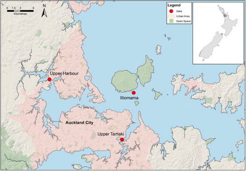
The main purpose of this study is to assess whether selected PSDs are capable of providing sufficient quality data for status and trend assessment of chemicals of current (heavy metals, PAHs) and emerging (EOCs) concern, as has previously been achieved by shellfish monitoring. Based on an assessment of the current literature, we chose PSDs applicable for the contaminant classes of interest. Polyethylene sampling devices (PED) were selected for hydrophobic contaminants (PAHs, polybrominated diphenyl ether [PBDE] flame retardants), diffusive gradients in thin films (DGT) were selected for heavy metals and polar organic chemical integrative samplers (POCIS) were selected for hydrophilic PPCP wastewater markers. Three study sites were selected to represent a gradient in contaminant levels, based on results from the former SCMP carried out by Auckland Council (Stewart et al. 2013a). Choosing sites that aligned with the former SCMP was critical to allow comparison of concentrations from PSDs with equivalent recent data from the SCMP. The sites chosen were Tamaki Estuary (heavily urbanised and industrial catchment), Upper Harbour (partly urbanised and partly rural catchment) and Illiomama Rock by Rangitoto Island (background site more removed from urban influences) (Figure 1).

Figure 1. Sites selected for PSD assessment. Tamaki Estuary is a heavily urbanised and industrial catchment, Upper Harbour is partly urbanised and partly rural catchment and Illiomama Rock is a background site more removed from urban influences.

Materials and methods

Passive sampling devices

PED were prepared from polyethylene sheets (50 μm nominal thickness), cropped to 85 × 2.5 cm strips, with a weight of approximately 1 g for each sampler. Each strip was sonicated in methylene chloride, acetone and Nanopure (18.2 MΩ) water, and then threaded onto stainless steel wire. Three strips were then secured inside a single metal g-minnow trap for deployment.

POCIS were self-fabricated, stainless steel encased ‘pharmaceutical’ configuration samplers. The configuration of each was consistent with commercially available POCIS, namely a 45.8 cm² sampling surface area (5.4 cm diameter opening), polyethersulfone membrane (Bioflow; 0.1 μm) and Oasis HLB (Waters Corp.) sorbent (200 mg). This resulted in a surface area to mass of sorbent ratio of approximately 180 cm²/g, consistent with the standard configuration of previously utilised POCIS (Alvarez et al. 2004). The POCIS were protected from large debris by an outer stainless steel mesh (3 mm diameter holes) and three of each POCIS were attached inside a single plastic burley cage (Anglers Mate) using cable ties.

Standard open pore DGT samplers were obtained commercially from DGT Research Ltd. Each DGT consisted of a stack of a hydrophilic 0.45 µm membrane filter disc (2.5 cm diameter) with typical thickness of 0.014 cm and a default 0.078 cm thick diffusive hydrogel layered on top of a standard 0.04 cm thick resin-embedded (Chelex-100) hydrogel enclosed tightly in robust plastic moulds with a round 2.0 cm diameter exposure window (Zhang 2003). Both hydrogels are composed of 15% acrylamide monomer and 0.3% agarose derivatives cross-linker (Zhang 2003; Warnken et al. 2005). Three DGTs per site were attached using cable ties to a plastic burley cage separate from the POCIS samplers.

Pictures of passive samplers used in this study are included in Figures S1–S3.

Deployment and retrieval

Samplers were contained in double zip-lock bags inside cooler bins until immediately prior to deployment, and then immediately after retrieval, to minimise potential contamination, for example by PAHs in vehicle and boat exhaust fumes. Note that the vessel engine was shutdown during deployment and retrieval. DGT samplers were removed from their plastic zip-lock bag immediately prior to deployment to ensure they did not dry out. Nine samplers (three replicates each of PED, POCIS and DGT) were deployed for between 20–21 days at each of the three sites in October/November 2014. A procedural blank of each was also included. Samplers were deployed at the Tamaki Estuary site by attaching to floating pontoons at Panmure Bridge Marina. At Upper Harbour and Illiomama sites, samplers were attached to channel markers and deployed and retrieved by boat and divers.

Water temperature, salinity and pH were measured during PSD deployment and retrieval. These parameters did not vary significantly between deployment and retrieval. Dissolved organic matter (DOM) was measured as dissolved organic carbon (DOC) at the University of Otago on water samples collected during deployment.

Upon retrieval, PEDs were removed from the water column, strips unthreaded from the wire and carefully wiped with Kimwipes (Kimberly-Clark) to remove surface detritus including fouling organisms and particulate matter (see Figures S1–S3). Strips were rolled carefully and placed inside original pre-cleaned scintillation vials, sealed and double zip-locked. POCIS were removed from their protective cage and double zip-locked. DGTs were removed from their protective cage, rinsed with deionised water, and double zip-locked in original bags.

Processing of PSDs

PEDs were placed in pre-cleaned 250 mL wide mouth amber jars. One clean PED was used as a quality control sample and was spiked with target analytes and the solvent allowed to evaporate. A second clean PED was used as a matrix blank. All PEDs were spiked with the PAH and PBDE internal standard mixtures (CARB 1997; USEPA 2007). Spiking was accomplished using a syringe to distribute the required volume of solution in small droplets deposited along the surface of the PED. The solvent from the spiking solutions was allowed to evaporate prior to extraction. Samples were extracted three times with dichloromethane (3 × 30 mL). Each extraction cycle involved 1 h on a table shaker at 200 rpm followed by 2 h standing. Solvent extracts were combined and adjusted to 100 mL final volume.

A 20% split was taken for PAH analysis, concentrated to 1 mL and cleaned up on a silica gel column (1 g). The extracts were concentrated to approximately 500 µL and spiked with recovery standard (CARB 1997). The extracts were transferred to a final volume of 500 µL iso-octane for analysis by gas chromatography-high resolution mass spectrometry (GC-HRMS). Results were corrected for internal standard recovery.

A 40% split was taken for brominated flame retardant (BFR) analysis, concentrated to 1 mL and cleaned up on a sulphuric acid impregnated silica gel column (1 g). The extracts were concentrated to approximately 500 µL and spiked with recovery standard (USEPA 2007). The extracts were transferred to a final volume of 100 µL toluene for analysis by GC-HRMS. Results were corrected for internal standard recovery.

The deployed POCIS were rinsed with reagent water to remove environmental debris before removing the sorbent. One clean POCIS was used as a quality control sample and was spiked with target analytes and the solvent allowed to evaporate. A second clean POCIS was used as a matrix blank. The sorbent was transferred to an empty polypropylene solid-phase extraction cartridge (6 mL) using reagent grade water and dried under vacuum. The sorbent was then spiked with internal standard and allowed to stand for 15 min prior to extraction with methanol (6 mL). Extracts were dried with anhydrous magnesium sulphate, centrifuged and made up to 10 mL with methanol. A 50% split was concentrated to approximately 400 µL, spiked with recovery standard and made up to 1 mL final volume for analysis by liquid chromatography-tandem mass spectrometry (LC-MS/MS). Results were corrected for internal standard recovery.

DGT were deconstructed and the sorbent layer leached for 24 h in 1 mL of 1 M high purity single-quartz distilled nitric acid. An internal standard was added and the leachate was diluted to a final acid concentration of 0.15 M nitric acid.

Analysis

PED extracts were analysed for 16 USEPA PAHs (Σ₁₆ USEPA PAH; Table 1), based on the GC-HRMS instrumental procedures of California Air Resources Board, Method 429 (CARB 1997).

Table 1. Physicochemical properties of hydrophobic contaminants analysed from polyethylene samplers.

	Water solubility (μg/L)^a	Molecular weight^a	log KOW^b	log KPED^b
PAHs
Naphthalene	31000	128.2	3.37	2.93
Acenaphthene	1930	154.2	3.98	3.62
Acenaphthylene	3930	152.2	4.07	2.79
Fluorene	1830	166.2	4.18	3.83
Phenanthrene	1200	178.2	4.45	4.21
Anthracene	76	178.2	4.45	4.17
Pyrene	77	202.3	4.88	4.58
Fluoranthene	230	202.3	4.90	4.75
Chrysene	2.8	228.3	5.16	5.41
Benz[a]anthracene	10	228.3	5.61	5.37
Benzo[b]fluoranthene	1.2	252.3	6.04	5.99
Benzo[a]pyrene	2.3	252.3	6.06	5.83
Benzo[k]fluoranthene	0.8	252.3	6.06	6.02
Benzo[g,h,i]perylene	0.3	276.3	6.50	6.25
Indeno(1,2,3-cd)pyrene	62	276.3	6.58	6.47
Dibenz[a,h]anthracene	0.5	278.4	6.84	6.46
PBDEs^c
BDE-15 (2)	130	328.0	5.82	5.04
BDE-28 (3)	70	406.9	6.24	5.30
BDE-47 (4)	15	485.8	6.80	6.23
BDE-99 (5)	9	564.7	7.38	6.81
BDE-153 (6)	1	643.6	7.86	7.38
BDE-183 (7)	2	722.5	8.61	7.83
BDE-209 (10)	0.1	959.2	9.87	5.36

^aPAH data taken from Agency for Toxic Substances and Disease Registry (ATSDR) (1995) or where not available USEPA (1996) or NCBI PubChem (http://www.ncbi.nlm.nih.gov/pccompound); PBDE data taken from ATSDR (2004).

^bPAH data from USEPA (2012); PBDE data from two sources (Bao et al. 2011; Perron et al. 2013).

^cFor brevity selected BDE congeners shown; number in brackets corresponds to number of bromine atoms.

BFRs were analysed by GC-HRMS, based on USEPA Method 1614 (USEPA 2007).

POCIS were analysed for 15 PPCP wastewater markers by LC-MS/MS. Analysis was performed using an Agilent 1290 HPLC with autosampler coupled to an ABSciex 5500QT Linear Ion Trap Quadrupole Tandem Mass Spectrometer equipped with a Turbo Spray ion source. The LC-MS/MS method utilised the multiple experiment feature of Analyst 1.6 to allow simultaneous positive and negative ionisation data acquisition, requiring only a single injection. Chromatographic separation was achieved on an Agilent XDB-C18 column (100 × 4.6 mm, 1.8 µm). Experimental conditions and performance statistics are summarised in Tables S1–S4. Calibration was performed using external standard methodology. Results were corrected for internal standard recovery. Absolute internal standard recovery was determined using ¹³C₈-perfluorooctanoic acid as a recovery standard. Multiple Reaction Monitoring (MRM) ratios for analytes in the samplers were required to be within ± 20% of those obtained in the calibration standards. Limits of reporting are summarised in Table S5.

DGT samplers were analysed for arsenic (As), cadmium (Cd), chromium (Cr), copper (Cu), iron (Fe), nickel (Ni), lead (Pb) and zinc (Zn) by inductively-coupled-plasma mass spectrometry (ICP-MS), using an Agilent 7500 cs/ce Quadrupole ICP-MS.

DOC was measured after filtration through acid-cleaned 0.45 um polyethersulfone (PES) membrane filters (Pall Corporation). The DOC was analysed as non-purgeable organic carbon (NPOC) using TOC analyser (Shimadzu V-CSH) in compliance with the Standard Method 5310 B. Approximately 35 mL of the filtered sample was transferred into pre-cleaned (soaked in pyroneg detergent and 2% v/v analytical grade hydrochloric acid [HCl]) and combusted (500 °C overnight) clear DOC vials and immediately acidified with concentrated (8 M) single quartz distilled HCl (prepared in-house inside a class 100 clean room) to a final concentration of 0.01 M (pH 2). The instrument was calibrated against six standard solutions (0–30 mg C/L standard solutions, acidified to pH 2) which were placed attentively in the batch analysis as a standard quality assurance/quality control routine procedure. The instrument was set to take three out of four best sample injection of 50 μL each which satisfy the standard deviation value of 0.1 and maximum coefficient of variation (CV) of 2%. In our analysis, the instrument’s calibration procedure was linear (r²= 0.9998) with a detection limit of 0.18 mg/L DOC.

Calculation of water concentrations

For POCIS, time-weighted average (TWA) water concentrations were calculated from equation (1), where C_W is the TWA concentration of the analyte in the water (μg/L), C_S is the concentration of the analyte in the sorbent (μg/g) at time t (days), M_S is the mass of sorbent in the POCIS (g) and R_S is the sampling rate (L/day):(1) R_S for many chemicals analysed from POCIS were derived (Morin et al. 2012) and incorporated into equation (1). Average and median sampling rates for all 15 wastewater marker analytes were calculated based on data from Morin et al. (2012) (Table 2). Data for ‘pesticide’ configuration POCIS, small surface area POCIS and calculated R_S were removed from calculations, unless these were the only data available. Where a saltwater R_S value was available, this was used in preference to other values.

Table 2. Comparison of calculated mean and median sampling rates (R_S) for wastewater chemicals analysed in POCIS samplers with log K_OW.

			RS (L/d)^a
Compound	Family	log KOW^b	n	Mean	SD	%RSD
Acetaminophen	Anti-inflammatory	0.91	4	0.266	0.269	101
Clarithromycin	Antibiotic	3.16	1^c	0.016	NA	NA
Caffeine	Stimulant	−0.13	3	0.125	0.028	22
Carbamazepine	Anticonvulsive	2.77	9	0.262	0.149	57
Diclofenac	Anti-inflammatory	4.26	3	0.124	0.034	27
Cotinine	Stimulant	−0.23	1	0.24	NA	NA
Benzophenone-2	UV filter	3.16	0^d	0.348	NA	NA
Benzophenone-3	UV filter	3.16	1	0.348	NA	NA
Ibuprofen	Anti-inflammatory	3.84	4	0.646	0.856	133
Triclosan	Disinfectant	4.8	6	0.91	0.697	77
Estriol (E3)	Hormone	2.67	1	0.12	NA	NA
Estrone (E1)	Hormone	4.31	1^c	0.15	NA	NA
β-Estradiol (β-E2)	Hormone	3.75	9	0.42	0.229	55
Ethynlestradiol (EE2)	Hormone	3.9	1^c	0.18	NA	NA
Bisphenol A (BPA)	Plasticiser	4.04	6	0.638	0.133	21

NA, not applicable.

^aR_S calculated from table 2 of Morin et al. (2012). However, pesticide POCIS values and small surface area rates were removed, where these were markedly different to other rates (estrone, β -E2, EE2, BPA).

^bFrom Morin et al. (2013), where available and ACD Labs where not (http://www.chemspider.com).

^cSingle saltwater value used.

^dValue for benzophenone-3 used.

For PED, the dissolved concentration (C_W: ng/L) was calculated using equation (2):(2) where C_S is the concentration of the contaminant in the passive sampler (ng contaminant/g sampler), and K_PED is the passive sampler-dissolved phase partition coefficient (L/kg). A multiplier of 1000 is included to address the change in units (g to kg). Values for a limited number of K_PED are available in the scientific literature. For PAHs, K_PED was taken from USEPA (2012), which were calculated from K_OW using the formula: log K_PED = 1.05 log K_OW–0.59 (Lohmann & Muir 2010), with K_OW the octanol-water partition coefficient (L/kg). For BDEs, an average K_PED was used from experimentally derived data from two studies (Bao et al. 2011; Perron et al. 2013). The effect of temperature and salinity on the sampler/water for hydrophobic compounds is small and can be corrected (Lohmann et al. 2012), but as these were very similar between sites no corrections were made.

The DGT-labile metal concentration (C_DGT) was calculated using equation (3) (Warnken et al. 2006; Davison & Zhang 2012):(3) where, M_DGT is the mass of metal accumulated in the resin hydrogel, t is the deployment time (s), A is the effective surface area of 3.8 cm², Δ_g is the diffusion layer thickness whereas D and D_w are diffusion of metal ions in the diffusive hydrogel and water at infinite dilution, respectively. Equation (4) was used to calculate M_DGT:(4) where C_ICPMS is the concentration of metals measured by ICMPS, V_HNO3 is the volume of nitric acid, V_resin is the volume of resin and f_e is the elution factor, which was standardised to 0.8 for all metals. The D for each metal was estimated by multiplying the metal ion’s D_w with the average ratio of D₂₅ /D_w, where D₂₅ is the D determined in solution with ionic strength of 0.1 mol L⁻¹ as NaNO₃ at 25 ˚C (Scally et al. 2006). The conversion of D₂₅ to D at in situ temperature was referred from Zhang & Davison (1995). Pb, Cr and As water concentrations are not reported due to non-specific elution factors (Pb, Cr) and unknown speciation (As).

Some contaminants were near the limit of quantitation (LOQ) and for any calculated water concentration to be reported, at least two of the three replicates needed to be above this limit. If only one replicate was quantified then the concentration was not reported. Where any contaminant was above the LOQ in control samplers, this value was subtracted from the deployed sampler concentrations.

Statistics

Statistical significance was assessed by an unpaired t-test, with significance regarded as P ≤ 0.05.

Results

PAHs

Calculated water concentrations of Σ₁₆ USEPA PAH were 8.9 ± 2.4 ng/L, 101.5 ± 8.1 ng/L and 6.3 ± 0.3 ng/L for Illiomama, Upper Harbour and Tamaki, respectively. Napthalene and acenapthylene were the largest contributors to total concentrations, with naphthalene highly variable between sites. Naphthlalene and phenanthrene concentrations were control subtracted. Σ₁₅ PAH were also calculated—which is the Σ₁₆ USEPA PAH list minus naphthalene—as it is applicable for comparison with other PAH data. Σ₁₅ PAH concentrations were 1.6 ± 0.1 ng/L, 20.4 ± 2.9 ng/L and 6.3 ± 0.3 ng/L for Illiomama, Upper Harbour and Tamaki, respectively. The Upper Harbour and Tamaki sites had significantly higher Σ₁₅ PAH concentrations than the background Illiomama site (P < 0.0005), with Upper Harbour also significantly higher than Tamaki (P < 0.001).

The concentrations of individual PAH congeners are presented in Figure 2, where hydrophilicity decreases from left to right. Figure 2 shows a clear relationship between PAH hydrophilicity and PED uptake, where uptake is biased towards more hydrophilic PAH congeners. All PAHs except dibenz[a,h]anthracene were detected from at least one site.

Figure 2. Calculated average (n = 3) PAH water concentrations from polyethylene samplers at three sites in the Waitemata Harbour. Error bars are ±1 SD about the mean. Inset: naphthalene, acenaphthene and acenaphthylene.

BDEs

Of the 40 BFRs analysed, only four BDE congeners (BDE-17, BDE-47, BDE-49 and BDE-209) were quantifiable and above control concentrations (Figure 3). BDE-47 was control subtracted due to quantifiable concentrations in the control. BDE-209 concentrations were up to 17.1 pg/L (parts-per-quadrillion) at Tamaki, while the lower brominated congeners had dissolved concentrations generally below 1 pg/L. The general concentration pattern was Illiomama < Upper Harbour < Tamaki (Figure 3).

Figure 3. Calculated average (n = 3) water concentrations for BDE congeners above detection limits from polyethylene samplers at three sites in the Waitemata Harbour. Error bars are ±1 SD about the mean. Inset: BDE-209.

PPCP wastewater markers

Of the 15 wastewater markers analysed, only three were quantified at all sites: paracetamol (acetaminophen); caffeine; and cotinine (Figure 4). Caffeine was quantified in control POCIS and so reported concentrations are control subtracted. Concentration ranges of 0.25–1.18 ng/L, 1.97–5.87 ng/L and 0.08–0.34 ng/L were observed for paracetamol, caffeine and cotinine, respectively (Figure 4). Increasing concentrations were observed Illiomama < Upper Harbour < Tamaki. These increases were significant between each site for caffeine and cotinine (P < 0.05), but only between Illiomama and Upper Harbour for paracetamol (P < 0.05). Triclosan and carbamazepine were detected at Upper Harbour only, with concentrations of 0.07 ng/L and 0.22 ng/L, respectively.

Figure 4. Calculated average (n = 3) water concentrations of wastewater markers from POCIS at three sites from the Waitemata Harbour. Error bars are ±1 SD about the mean.

Metals

Calculated labile dissolved concentrations of Zn, Cu, Fe, Ni and Cd are presented in Figure 5. The highest concentrations observed were for Zn, ranging from 0.52–5.43 μg/L. Other metal concentration ranges were 0.29–1.87 μg/L (Fe), 0.13–0.31 μg/L (Ni), 0.09–0.55 μg/L (Cu) and 0.009–0.120 μg/L (Cd), respectively.

Figure 5. Calculated average (n = 3) labile zinc, copper, iron, nickel and cadmium water concentrations at three sites from Waitemata Harbour. Error bars are ±1 SD about the mean.

Zn and Cu generally showed significant concentration increases (P < 0.05) from Illiomama < Upper Harbour < Tamaki, with the exception of Cu, which was not significantly different between Upper Harbour and Tamaki (P = 0.32). Fe and Ni concentrations showed a significant (P < 0.05) pattern of Illiomama < Tamaki < Upper Harbour. For Cd, concentrations were only significantly different between Upper Harbour and Tamaki (P < 0.01).

DOC concentrations were 2.40 mg/L, 2.32 mg/L and 0.76 mg/L for Upper Harbour, Tamaki and Illiomama, respectively (i.e. showing similar trends as other organic and trace metal contaminants).

Discussion

Study limitations

The accuracy of calculated water concentrations from PSDs depends on establishing equilibrium conditions for PED and using field corrected sampling rates (R_S) for POCIS. Correction for non-equilibrium conditions is usually achieved by use of performance reference compounds (PRCs). Unless equilibrium conditions are achieved, not using PRCs will generally result in an underestimation of the water concentration (Perron et al. 2013). The use of PRCs is logistically complex and they were not used in this study; therefore, results presented here for PED may underestimate actual concentrations.

POCIS sampling rates are often derived in the laboratory; however, variables such as flow, temperature, biofouling and pH can affect sampling rates under field conditions (Harman et al. 2012). The use of PRCs in POCIS is under investigation (e.g. Morin et al. 2012; Vallejo et al. 2013; Belles et al. 2014); however, consensus has not been reached at this stage as to their suitability (Harman et al. 2011; Vallejo et al. 2013). As such, sampling rates used for each analyte in this study were largely averages of multiple studies (where available). In practice, high variability in reported sampling rates is observed for some analytes. For example the sampling rate for acetaminophen has a percent relative standard deviation (%RSD) of 101% (Table 2). This suggests that, in the absence of sampling rate data for specific local conditions, calculating average sampling rates is a valid approach. For the three wastewater markers quantified, there is an inherent 2-fold variability in water concentrations of acetaminophen, whereas an acceptable %RSD of 22% was calculated for caffeine, suggesting higher confidence in the water concentration. It was not possible to assess sampling rate variability for cotinine as it was based on only one literature value.

Similar assumptions used for POCIS also apply to DGTs, regarding a constant flow, temperature and pH, all of which have influence on the trace metal speciation. DOM may also have a large effect in the labile form of trace metals. However, we measured DOC as a surrogate for DOM with concentrations expected to specific locations (i.e. background sample Illiomama receiving most clean seawater showed lowest DOC). Upper Harbour and Tamaki would both receive more riverine DOM/DOC. The trace metal binding capacity at the three sites was not analysed during this study, but might be useful in the future to explain differences in bioavailability pattern between Upper Harbour and Tamaki.

The main objective of this study was to assess whether PSDs are capable of providing data that would establish concentration gradients across three sites of differing urban influence (see Figure 1). As concentrations of contaminants in these environments are within an order of magnitude, and most other environmental conditions were similar or controlled as best as was practicable, it was considered that bioavailable concentrations provided by PSDs would be sufficient in this instance in achieving the main aims. However, any future studies should include PRCs and environmental sampling rates to more accurately establish contaminant concentrations.

PAHs

The concentrations of 15 PAHs (minus naphthalene) calculated from PED were compared with the most current mussel tissue data (2010–2013 medians) (Figure 6). The congener profile in mussels is relatively evenly spread across the 15 congeners, with possible bias towards more hydrophobic PAHs. In contrast, water PAH concentrations calculated from PEDs are biased predominantly towards more hydrophilic PAHs. This is not surprising as mussels will also ingest and accumulate more hydrophobic PAHs associated with suspended particulate matter, whereas PEDs only adsorb the dissolved portion.

Figure 6. Comparison of mussel and PED uptake of PAHs. PAHs have been sorted (left to right) by decreasing hydrophilicity.

Uptake of Σ₁₅ PAH is not consistent between PED and mussels, with a weak correlation observed between the two (R² = 0.25, data not shown). However, as is consistent with Alvarez et al. (2014b), when only three hydrophobic PAHs (benzo[a]pyrene, benzo[g,h,i]perylene and chrysene) are compared, there was a strong correlation (R² = 0.94–1.00, data not shown) between water concentration and mussel tissue concentration. This suggests these three PAHs could be used as representative markers for mussel tissue PAH concentrations.

To our knowledge, this is the first report of PAH concentrations calculated from PSDs in New Zealand. International studies reporting dissolved concentrations of PAHs from PSDs in estuarine environments are not prevalent. For published studies there is little consistency in passive sampling methodologies used, congeners analysed and study aims; however, limited comparisons may be made. The calculated Σ₁₅ PAH concentrations from this study (1.6–20.4 ng/L) are lower but comparable with Perron et al. (2013) who reported Σ₁₅ PAH concentrations of 14.4–35.3 (median 23.1) ng/L from PEDs at six sites in a temperate estuary in Rhode Island, USA. A study assessing the environmental impact of aquatic discharges from the offshore oil industry in Norway (Harman et al. 2009) reported Σ₁₅ PAH concentrations of 1.7–4.5 ng/L using semipermeable membrane devices (SPMDs) instead of PEDs. Alvarez et al. (2014a) reported Σ₅ PAH (chrysene, dibenzo[a,h]anthracene, indeno[1,2,3-cd]pyrene, benzo[g,h,i]perylene, benzo[a]pyrene) concentrations of 0.001–6.8 (mean 0.7) ng/L from PEDs along the Californian coast, which were markedly higher than Σ₅ PAH of 0.015–0.046 ng/L for this study. These findings suggest PAH concentrations in the Waitemata Harbour are within the range of those in other marine environments.

The Australian and New Zealand Environment and Conservation Council (ANZECC) have set ecological marine water trigger values for a range of contaminants. Naphthalene, anthracene, phenanthrene, fluoranthene and benzo[a]pyrene have been included by ANZECC as they show possible bioaccumulation and secondary poisoning effects; however, trigger values have been set for naphthalene only, with 50 μg/L set as the most protective (99%) marine ecological trigger value. The highest concentration of naphthalene in this study (0.08 μg/L at Upper Harbour) is orders of magnitude below this trigger value. Benzo[a]pyrene, benzo[b]fluoranthene, benzo[g,h,i]perylene, benzo[k]fluoranthene and indeno[1,2,3-cd]pyrene have been listed as priority hazardous substances in Annex X under the EU Water Framework Directive (European Commission 2013). It was acknowledged in this directive that benzo[a]pyrene can be considered as a marker for the other PAHs and only benzo[a]pyrene needs to be monitored for comparison with annual average environmental quality standards (AA-EQS). Any contaminant concentration below the EQS suggests good surface water chemical status for that contaminant (European Commission 2000). For benzo[a]pyrene, AA-EQS is 0.17 μg/L, which is 30-fold higher than the maximum average concentration of benzo[a]pyrene from this study. This suggests marine water concentrations at the three sites sampled have good status with respect to dissolved PAHs, even if the method used here may be underestimating actual PAH concentrations.

BDEs

BDE concentrations were generally below 1 pg/L, when decabrominated diphenyl ether (BDE-209) was not included in the total calculations. This is at the lower end of other relevant studies. Alvarez et al. (2014a) reported mean individual BDE congener water concentrations (not including BDE-209) of between 0.008–4.3 pg/L along the Californian coast, while Perron et al. (2013) reported Σ₅ BDE concentrations of 13.1–62.2 pg/L. Interestingly, Perron’s study analysed for BDE-209, but did not report water concentrations of this congener as they did not observe a good relationship between log K_OW and log K_PED. It has been shown that a linear relationship is observed between log K_OW and log K_PED until a plateau at log K_OW of approximately 8.3 is reached, above which any further increase in log K_OW corresponds to a decrease in log K_PED (Bao et al. 2011). BDE209 has a log K_OW of 9.87 (Table 1). Despite these reservations, BDE-209 has been reported from this study as it was detected well above control levels at two out of three sites and is the most abundant BDE congener encountered in marine sediments around Auckland (Stewart et al. 2014).

There are currently no ANZECC guidelines to assess ecological risk of BDEs. BDE congener numbers 28, 47, 99, 100, 153 and 154 have been listed as priority hazardous substances in Annex X under the EU Water Framework Directive (European Commission 2013), with maximum allowable concentration environmental quality standards (MAC-EQS) of 140 ng/L and 14 ng/L for inland surface waters (lakes and rivers) and other surface waters, respectively. The EQS refers to the sum of the concentrations (total in the whole water sample) of the six BDE congeners listed as priority hazardous substances. Of these, only BDE-47 was detected in this study and at levels between 10⁵- and 10⁶-fold lower than MAC-EQS, suggesting negligible environmental risk of dissolved BDEs at the three sites sampled, even if the method used here may be underestimating actual BDE concentrations.

The concentrations of BDEs in this study (pg/L, or parts-per-quadrillion) are around three orders of magnitude lower than PAH concentrations (ng/L, or parts-per-trillion). This is not surprising, as BDEs are generally considerably less hydrophilic than PAHs, with log K_OW 5.82–9.87 and log K_OW 3.37–6.84 for BDEs and PAHs, respectively (Table 1). As such, BDEs are likely to have much stronger association with particulates than water. Furthermore, sources of PAHs (both pyrogenic and petrogenic) are likely manifold higher than BDEs (industrial and residential stormwater and wastewater discharges, landfill leachate), which would likely be reflected in higher environmental concentrations.

A comparison of BDE and PAH concentrations in sediment from the Auckland region suggests the ratio is similar to water concentrations; that is, an approximate three orders of magnitude higher concentration of PAHs (low mg/kg; Mills et al. 2012) than BDEs (low μg/g; Stewart et al. 2014). These results suggest—despite the marked difference in solubility between PAHs and BDEs—that environmental concentrations of PAHs are approximately three orders of magnitude higher than BDEs in the Auckland estuarine environment, regardless of the receiving phase (water or sediment). As yet concentrations of BDEs in estuarine biota and bioaccumulation relationships have not been investigated in New Zealand.

PPCPs

Five anthropogenic chemical markers were detected in the Auckland marine environment, with three of these (paracetamol, caffeine and cotinine) showing a general significant incremental increase in concentration from Illiomama (background site) to Upper Harbour (partial urban) and Tamaki (fully urban/industrial).

Caffeine concentrations in this study (2–6 ng/L) are lower, but similar to those reported from POCIS studies in Mediterranean coastal waters (8–32 ng/L; Munaron et al. 2012) and along the California coast (mean 10 ng/L; Alvarez et al. 2014a). Cotinine concentrations (0.14–0.59 ng/L) are lower, but similar to the Californian study (mean 2.7 ng/L). Interestingly, paracetamol (acetaminophen) was detected at all three sites from this study (0.25–1.18 ng/L), but was not detected at any sites in the California study (Alvarez et al. 2014a).

Parameters such as flow, pH and temperature have been shown to affect sampling kinetics for a range of polar chemicals (e.g. Li et al. 2011, 2010; Charlestra et al. 2012; Morin et al. 2013; Dalton et al. 2014). Between the three sites in this study, pH and temperature were virtually the same, so flow is likely to be the largest influence on uptake kinetics. All three sites are tidally influenced, so for most of the time flow is similar as samplers were placed in maximum flow. Furthermore, flow rates have been shown to have little influence on cotinine and caffeine uptake on POCIS (Li et al. 2010). As such, it is valid to compare concentrations between sites in this case, and POCIS show a clear ability to differentiate selected wastewater markers. Furthermore, the contaminant suite can be expanded in future to include other hydrophilic wastewater markers of interest (e.g. artificial sweeteners).

To our knowledge there are no reports of PPCP wastewater markers in shellfish in New Zealand. As such it is not possible to compare POCIS results from this study with relevant national results. However, insight can be gained from international studies. In a pilot study to refocus the US Mussel Watch Program to contaminants of emerging concern (Dodder et al. 2014; Alvarez et al. 2014a; Maruya et al. 2014a), it was shown that there was very little overlap (one out of 40 analytes) between POCIS and mussel tissue. The authors noted that, generally, chemicals detected in mussels had log K_OW > 3, whereas those from POCIS had log K_OW < 3 (Alvarez et al. 2014a). As such, mussels appear to be poor biomonitors of polar organic chemicals and passive samplers have a clear advantage in this regard.

Metals

Strong positive correlations were observed for Zn, Cu and Cd (R² = 0.68, 0.83 and 0.96, respectively) between DGT and mussel tissue concentrations (2010–2013 medians) (Figure 7), suggesting that DGTs are good surrogates for mussels regarding these three key urban metals. However, data variance of DGTs (three replicates) from this study is higher than the most recent mussel data (three replicates, 2013 data). DGT coefficient of variation (CV%) ranged from 7% to 22% for the five reported metals, whereas CV% for mussel metal tissue data (Cu, Zn, Cd only) was less than 6%. Despite the larger variance in DGT-derived metal water concentrations, generally significant differences in concentrations were observed between sites (Figure 5).

Figure 7. Correlations between shellfish metal concentrations (2010–2013: median) and calculated labile water concentrations for three study sites in the Waitemata Harbour.

DGTs not only provide time-weighted average (TWA) metal water concentrations, they also afford extremely low detection limits (DLs), well below currently available dissolved seawater concentration DLs of 0.2 μg/L (Cd), 1 μg/L (Cr, Cu, Ni) and 4 μg/L (Fe, Zn) (Gadd & Cameron 2012; Hill Laboratories 2014). Current dissolved metal seawater DLs provide data sufficient to compare with trigger values for 95% species protection (ANZECC 2000) for the five metals reported in this study. Therefore, the major advantage of DGTs over grab sampling is that they provide TWA metal concentrations.

Conclusions

This study was designed to assess whether PSDs could replace or complement shellfish in establishing concentration gradients between a background site (Illiomama), distant from many anthropogenic inputs, a site within a partially urbanised catchment (Upper Harbour), and a site within a fully urbanised and industrialised catchment (Tamaki). It is acknowledged that with three sites it is difficult to obtain robust statistical data. However, three replicates of each PSD were usually sufficient to reveal inter-site differences.

PSDs offer certain advantages and disadvantages to shellfish monitoring. Although it is premature to make conclusions as to the suitability of PSDs in replacing shellfish until more information is available, the results show that PSDs can currently complement shellfish in SoE monitoring programmes. PSDs can be used for other applications, such as an alternative to grab water sampling in water quality assessments. PSDs offer two significant advantages over grab water sampling: lower detection limits; and time-weighted average concentrations. Lower detection limits provide greater flexibility, while time-weighted average concentrations reduce effects of short-term fluctuations in water concentrations and are more applicable to chronic guidelines, such as those set by ANZECC.

PSDs are currently undergoing intensive research to assess what requirements are necessary before they can be used in regulatory monitoring, with the general consensus being that they require more research before they can be implemented (Jones et al. 2015; Miège et al. 2015; Vrana et al. 2016; Roll & Halden, 2016).

Supplementary data

Dataset S1. Pictures of each PSD type on retrieval and summary of analytical methodology used for measurement of contaminants.

Figure S1. Picture (on retrieval) of DGT deployed in plastic burley cage for protection.

Figure S2. Picture (on retrieval) of POCIS. These were deployed in plastic burley cage (separate to DGT) for protection.

Figure S3. Picture (on retrieval) of PED deployed in metal fish cage for protection.

Table S1. LC gradient.

Table S2. MS/MS parameters.

Table S3. Internal standard recovery statistics.

Table S4. Analyte recovery from spiked sampler.

Table S5. Limit of reporting (LOR) for POCIS sampler.

Acknowledgements

We thank Melanie Vaughan (Auckland Council) for help with GIS mapping.

Associate Editor: Associate Professor Conrad Pilditch.

Disclosure statement

No potential conflict of interest was reported by the authors.

ORCID

M Stewart http://orcid.org/0000-0002-7035-4483

Additional information

Funding

The authors acknowledge the following funding sources: NIWA for project design, sampling and analyses (Core funding project [Grant number: FWWQ1504]); Auckland Council for in-kind support and funding for analyses and manuscript; and Streamlined Environmental (Core funding for manuscript).

References

- Alvarez DA, Maruya KA, Dodder NG, Lao W, Furlong ET, Smalling KL. 2014a. Occurrence of contaminants of emerging concern along the California coast (2009–10) using passive sampling devices. Mar Poll Bull. 81:347–354. doi: 10.1016/j.marpolbul.2013.04.022
- Alvarez DA, Perkins S, Nilsen E, Morace J. 2014b. Spatial and temporal trends in occurrence of emerging and legacy contaminants in the Lower Columbia River 2008–2010. Sci Total Environ. 484:322–330. doi: 10.1016/j.scitotenv.2013.07.128
- Alvarez DA, Petty JD, Huckins JN, Jones-Lepp TL, Getting DT, Goddard JP, Manahan SE. 2004. Development of a passive, in situ, integrative sampler for hydrophilic organic contaminants in aquatic environments. Environ Toxic Chem. 23:1640–1648. doi: 10.1897/03-603
- ANZECC. 2000. Australian and New Zealand guidelines for fresh and marine water quality. Volume 1. Canberra, ACT: Australian and New Zealand Environment and Conservation Council; Agriculture and Resource Management Council of Australia and New Zealand.
- Arp HPH. 2012. Emerging decontaminants. Environ Sci Technol. 46:4259–4260. doi: 10.1021/es301074u
- [ATSDR] Agency for Toxic Substances and Disease Registry. 1995. Toxicological profile for polycyclic aromatic hydrocarbons (PAHs). Atlanta, GA: US Department of Health and Human Services, Public Health Service.
- [ATSDR] Agency for Toxic Substances and Disease Registry. 2004. Toxicological profile for polybrominated biphenyls and polybrominated diphenyl ethers. Atlanta, GA: US Department of Health and Human Services, Public Health Service.
- Bao L, You J, Zeng EY. 2011. Sorption of PBDE in low-density polyethylene film: implications for bioavailability of BDE-209. Environ Toxic Chem. 30:1731–1738. doi: 10.1002/etc.564
- Belles A, Tapie N, Pardon P, Budzinski H. 2014. Development of the performance reference compound approach for the calibration of ‘polar organic chemical integrative sampler’ (POCIS). Anal Bioanal Chem. 406:1131–1140. doi: 10.1007/s00216-013-7297-z
- Cameron M, Stewart M, Gadd J, Ballantine D, Olsen G. 2014. The end of an era: what patterns have been revealed as 26 years of shellfish contaminant monitoring in Auckland comes to an end? Presented at: New Zealand Marine Sciences Conference, Nelson.
- CARB. 1997. Method 429. Determination of polycyclic aromatic hydrocarbon (PAH) emissions from stationary sources. Sacramento, CA: Air Resources Board, California Environmental Protection Agency.
- Charlestra L, Amirbahman A, Courtemanch DL, Alvarez DA, Patterson H. 2012. Estimating pesticide sampling rates by the polar organic chemical integrative sampler (POCIS) in the presence of natural organic matter and varying hydrodynamic conditions. Environ Poll. 169:98–104. doi: 10.1016/j.envpol.2012.05.001
- Dalton RL, Pick FR, Boutin C, Saleem A. 2014. Atrazine contamination at the watershed scale and environmental factors affecting sampling rates of the polar organic chemical integrative sampler (POCIS). Environ Poll. 189:134–142. doi: 10.1016/j.envpol.2014.02.028
- Daughton CG. 2002. Environmental stewardship and drugs as pollutants. The Lancet. 360:1035–1036. doi: 10.1016/S0140-6736(02)11176-7
- Davison W, Zhang H. 2012. Progress in understanding the use of diffusive gradients in thin films (DGT)—back to basics. Environ Chem. 9:1–3. doi: 10.1071/EN11084
- Dodder NG, Maruya KA, Lee Ferguson P, Grace R, Klosterhaus S, La Guardia MJ, Lauenstein GG, Ramirez J. 2014. Occurrence of contaminants of emerging concern in mussels (Mytilus spp.) along the California coast and the influence of land use, storm water discharge, and treated wastewater effluent. Mar Poll Bull. 81:340–346. doi: 10.1016/j.marpolbul.2013.06.041
- European Commission. 2000. Directive 2000/60/EC of The European Parliament and of The Council of 23 October 2000 establishing a framework for community action in the field of water policy. Luxembourg: European Parliament, Council of the European Union; [cited 2016 Apr 20]. Available from: http://eur-lex.europa.eu/legal-content/EN/TXT/?uri=celex%3A32000L0060
- European Commission. 2013. Directive 2013/39/EU of The European Parliament and of The Council of 12 August 2013 amending Directives 2000/60/EC and 2008/105/EC as regards priority substances in the field of water policy. Text with EEA relevance. Luxembourg: European Parliament, Council of the European Union; [cited 2016 Apr 20]. Available from: http://eur-lex.europa.eu/legal-content/EN/ALL/?uri=CELEX%3A32013L0039
- Gadd J, Cameron M. 2012. Antifouling biocides in marinas: measurement of copper concentrations and comparison to model predictions for eight Auckland sites. Auckland Council Technical Report TR2012/033. Auckland: Auckland Council.
- Ghosh U, Kane Driscoll S, Burgess RM, Jonker MTO, Reible D, Gobas F, Choi Y, Apitz SE, Maruya KA, Gala WR, et al. 2014. Passive sampling methods for contaminated sediments: practical guidance for selection, calibration, and implementation. Integr Environ Assess Manag. 10:210–223. doi: 10.1002/ieam.1507
- Greenwood R, Mills G, Vrana B, editors. 2007. Passive sampling techniques in environmental monitoring. Comprehensive Analytic Chemistry, volume 48. Amsterdam, The Netherlands: Elsevier.
- Harman C, Allan IJ, Vermeirssen ELM. 2012. Calibration and use of the polar organic chemical integrative sampler—a critical review. Environ Toxic Chem. 31:2724–2738. doi: 10.1002/etc.2011
- Harman C, Brooks S, Sundt RC, Meier S, Grung M. 2011. Field comparison of passive sampling and biological approaches for measuring exposure to PAH and alkylphenols from offshore produced water discharges. Mar Poll Bull. 63:141–148. doi: 10.1016/j.marpolbul.2010.12.023
- Harman C, Thomas KV, Tollefsen KE, Meier S, Bøyum O, Grung M. 2009. Monitoring the freely dissolved concentrations of polycyclic aromatic hydrocarbons (PAH) and alkylphenols (AP) around a Norwegian oil platform by holistic passive sampling. Mar Poll Bull. 58:1671–1679. doi: 10.1016/j.marpolbul.2009.06.022
- Hill Laboratories. 2014. Environmental catalogue V9.0. Hamilton: Hill Laboratories; [cited 2016 Apr 20]. Available from: http://www.hill-laboratories.com/file/fileid/50317
- Jones L, Ronan J, McHugh B, McGovern E, Regan F. 2015. Emerging priority substances in the aquatic environment: a role for passive sampling in supporting WFD monitoring and compliance. Anal Methods. 7:7976–7984. doi: 10.1039/C5AY01059D
- Li H, Helm PA, Paterson G, Metcalfe CD. 2011. The effects of dissolved organic matter and pH on sampling rates for polar organic chemical integrative samplers (POCIS). Chemosphere. 83:271–280. doi: 10.1016/j.chemosphere.2010.12.071
- Li H, Vermeirssen ELM, Helm PA, Metcalfe CD. 2010. Controlled field evaluation of water flow rate effects on sampling polar organic compounds using polar organic chemical integrative samplers. EnvironToxic Chem. 29:2461–2469.
- Lohmann R, Booij K, Smedes F, Vrana B. 2012. Use of passive sampling devices for monitoring and compliance checking of POP concentrations in water. Environ Sci Poll Res. 19:1885–1895. doi: 10.1007/s11356-012-0748-9
- Lohmann R, Muir D. 2010. Global aquatic passive sampling (AQUA-GAPS): using passive samplers to monitor POPs in the waters of the world. EnvironSci Tech. 44:860–864. doi: 10.1021/es902379g
- Maruya KA, Dodder NG, Schaffner RA, Weisberg SB, Gregorio D, Klosterhaus S, Alvarez DA, Furlong ET, Kimbrough KL, Lauenstein GG, Christensen JD. 2014a. Refocusing Mussel Watch on contaminants of emerging concern (CECs): the California pilot study (2009–10). Mar Poll Bull. 81:334–339. doi: 10.1016/j.marpolbul.2013.04.027
- Maruya KA, Dodder NG, Weisberg SB, Gregorio D, Bishop JS, Klosterhaus S, Alvarez DA, Furlong ET, Bricker S, Kimbrough KL, Lauenstein GG. 2014b. The Mussel Watch California pilot study on contaminants of emerging concern (CECs): synthesis and next steps. Mar Poll Bull. 81:355–363. doi: 10.1016/j.marpolbul.2013.04.023
- Miège C, Mazzella N, Allan I, Dulio V, Smedes F, Tixier C, Vermeirssen E, Brant J, O’Toole S, Budzinski H, et al. 2015. Position paper on passive sampling techniques for the monitoring of contaminants in the aquatic environment—achievements to date and perspectives. Trends Analyt Chem. 8:20–26. doi: 10.1016/j.teac.2015.07.001
- Mills G, Williamson B, Cameron M, Vaughan M. 2012. Marine sediment contaminants: status and trends assessment 1998 to 2010. Auckland Council Technical Report TR2012/041. Auckland: Auckland Council.
- Morin N, Camilleri J, Cren-Olivé C, Coquery M, Miège C. 2013. Determination of uptake kinetics and sampling rates for 56 organic micropollutants using ‘pharmaceutical’ POCIS. Talanta. 109:61–73. doi: 10.1016/j.talanta.2013.01.058
- Morin N, Miège C, Coquery M, Randon J. 2012. Chemical calibration, performance, validation and applications of the polar organic chemical integrative sampler (POCIS) in aquatic environments. Trends Analyt Chem. 36:144–175. doi: 10.1016/j.trac.2012.01.007
- Munaron D, Tapie N, Budzinski H, Andral B, Gonzalez JL. 2012. Pharmaceuticals, alkylphenols and pesticides in Mediterranean coastal waters: results from a pilot survey using passive samplers. Estuar Coast Shelf Sci. 114:82–92. doi: 10.1016/j.ecss.2011.09.009
- Perron MM, Burgess RM, Suuberg EM, Cantwell MG, Pennell KG. 2013. Performance of passive samplers for monitoring estuarine water column concentrations 1. Contaminants of concern. EnvironToxic Chem. 32:2182–2189.
- Roll IB, Halden RU. 2016. Critical review of factors governing data quality of integrative samplers employed in environmental water monitoring. Water Res. 94:200–207. doi: 10.1016/j.watres.2016.02.048
- Scally S, Davison W, Zhang H. 2006. Diffusion coefficients of metals and metal complexes in hydrogels used in diffusive gradients in thin films. Anal Chim Acta. 558:222–229. doi: 10.1016/j.aca.2005.11.020
- Stewart M, Gadd J, Ballantine D, Olsen G. 2013a. Shellfish contaminant monitoring programme: status and trends analysis 1987–2011. Auckland Council Technical Report TR2013/054. Auckland: Auckland Council.
- Stewart M, Olsen G, Gadd J. 2013b. Shellfish contaminant monitoring programme review. Auckland Council Technical Report, TR2013/055. Auckland: Auckland Council.
- Stewart M, Olsen G, Hickey CW, Ferreira B, Jelić A, Petrović M, Barcelo D. 2014. A survey of emerging contaminants in the estuarine receiving environment around Auckland, New Zealand. Sci Total Environ. 468–469:202–210. doi: 10.1016/j.scitotenv.2013.08.039
- [UNEP] United Nations Environment Programme. 2009. Stockholm Convention on persistent organic pollutants (POPs) as amended in 2009. Text and Annexes. Rotterdam, Switzerland: UNEP.
- [USEPA] US Environmental Protection Agency. 1996. Soil screening guidance: technical background document. Part 5: Chemical-specific parameters. Washington, DC: Office of Solid Waster and Emergency Response, EPA.
- [USEPA] US Environmental Protection Agency. 2007. Method 1614. Brominated diphenyl ethers in water soil, sediment and tissue by HRGC/HRMS. Washington, DC: Office of Water, EPA.
- [USEPA] US Environmental Protection Agency. 2012. Equilibrium partitioning sediment benchmarks (ESBs) for the protection of benthic organisms: procedures for the determination of the freely dissolved interstitial water concentrations of nonionic organics. EPA-600-R-02–012. Washington, DC: Office of Research and Development, EPA.
- Vallejo A, Prieto A, Moeder M, Usobiaga A, Zuloaga O, Etxebarria N, Paschke A. 2013. Calibration and field test of the polar organic chemical integrative samplers for the determination of 15 endocrine disrupting compounds in wastewater and river water with special focus on performance reference compounds (PRC). Water Res. 47:2851–2862. doi: 10.1016/j.watres.2013.02.049
- Vrana B, Allan IJ, Greenwood R, Mills GA, Dominiak E, Svensson K, Knutsson J, Morrison G. 2005. Passive sampling techniques for monitoring pollutants in water. Trends Anal Chem. 24:845–868. doi: 10.1016/j.trac.2005.06.006
- Vrana B, Smedes F, Prokeš R, Loos R, Mazzella N, Miege C, Budzinski H, Vermeirssen E, Ocelka T, Gravell A, Kaserzo S. 2016. An interlaboratory study on passive sampling of emerging water pollutants. Trends Anal Chem. 76:153–165. doi: 10.1016/j.trac.2015.10.013
- Warnken KW, Zhang H, Davison W. 2005. Trace metal measurements in low ionic strength synthetic solutions by diffusive gradients in thin films. Anal Chem. 77:5440–5446. doi: 10.1021/ac050045o
- Warnken KW, Zhang H, Davison W. 2006. Accuracy of the diffusive gradients in thin-films technique: diffusive boundary layer and effective sampling area considerations. Anal Chem. 78:3780–3787. doi: 10.1021/ac060139d
- Zhang H. 2003. DGT-for measurements in waters, soils and sediments. Lancaster, UK: DGT Research Ltd.
- Zhang H, Davison W. 1995. Performance characteristics of diffusion gradients in thin films for the in situ measurement of trace metals in aqueous solution. Anal Chem. 67:3391–3400. doi: 10.1021/ac00115a005