Climate change projections for the surface ocean around New Zealand

ABSTRACT

The future status of the surface ocean around New Zealand was projected using two Earth System Models and four emission scenarios. By 2100 mean changes are largest under Representative Concentration Pathway 8.5 (RCP8.5), with a +2.5°C increase in sea surface temperature, and decreases in surface mixed layer depth (15%), macronutrients (7.5–20%), primary production (4.5%) and particle flux (12%). Largest macronutrient declines occur in the eastern Chatham Rise and subantarctic waters to the south, whereas dissolved iron increases in subtropical waters. Surface pH projections, validated against subantarctic time-series data, indicate a 0.335 decline to ∼7.77 by 2100. However, projected pH is sensitive to future CO₂ emissions, remaining within the current range under RCP2.6, but decreasing below it by 2040 with all other scenarios. Sub-regions vulnerable to climate change include the Chatham Rise, polar waters south of 50°S, and subtropical waters north of New Zealand, whereas the central Tasman Sea is least affected.

KEYWORDS:

• Climate change
• surface ocean
• New Zealand
• Earth System Model
• warming
• ocean acidification
• nutrients
• primary production
• particle flux

Introduction

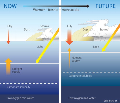
There is increasing awareness that climate change is altering the physical and biogeochemical status of the surface ocean, potentially impacting marine ecosystems and, consequently, the benefits and services they provide (Bopp et al. 2013; Weatherdon et al. 2016; Sweetman et al. 2017). The recent IPCC assessment identified that a number of physical and biogeochemical properties of the upper ocean are changing (Pörtner et al. 2014; see Figure 1), raising concerns regarding the stability of marine foodwebs and ecosystems. The oceans contain 93% of the additional global heat arising from increasing greenhouse gas concentrations (Levitus et al. 2012), and consequently increasing ocean temperature is a primary feature of climate change in marine ecosystems. Warming and associated changes in ocean dynamics have been identified as the drivers of an increase in the surface area of the oligotrophic ocean (Polovina et al. 2011), and regional shifts in abundance and distribution of marine biotic groups (Poloczanska et al. 2013). The resulting poleward and depth migration of species may alter ecosystem structure and species interactions, with implications for food and economic security in tropical and subtropical regions (Hoegh-Guldberg et al. 2014). Warming also increases upper ocean stratification, which affects light and nutrient availability (Riebesell et al. 2009, see Figure 1), and consequently influences phytoplankton growth. The uptake of anthropogenic CO₂ also leads to a decrease in pH and associated changes in water chemistry that may impact various biotic groups, particularly carbonate-forming species (Kroecker et al. 2013; Law et al. 2017). The individual and interactive effects of these climate-modulated controls will alter phytoplankton productivity, distribution and biodiversity, and so impact marine food webs via changes in the quantity and quality of organic matter, with implications for ecosystems, fisheries and the ocean carbon sink.

Figure 1. Conceptual figure of the projected changes in upper ocean properties in response to climate change (reproduced from Boyd and Law 2011). The magnitude of future change is projected for some of these factors whereas others, such as dust and storm events, are not considered in this paper.

Despite the ocean dominating the New Zealand (NZ) Exclusive Economic Zone (EEZ), with the landmass occupying only ∼7%, the response of marine ecosystems to climate change is largely unknown. Located in the South-West Pacific (SWP) between 22°S and 55°S the EEZ straddles the boundary between subtropical and subantarctic water masses of contrasting physico-biogeochemical characteristics. Consequently, NZ sits at an interface, between subtropical waters characterised by low nutrients and productivity, both of which are projected to decline further, and subantarctic waters in which productivity may increase (Bopp et al. 2013; Rickard et al. 2016). Whereas warming increases stratification, and poleward advection may increase the proportion of lower productivity oligotrophic water in the EEZ, a poleward shift in primary production and species distribution (Cheung et al. 2012) may be beneficial to temperate and subantarctic waters around NZ. However, this poleward shift may also increase the transfer of invasive species and disease (see references in Weatherdon et al. 2016). From an economic perspective, NZ has a productive seafood industry, with an annual harvest of 600,000 tonnes and export earnings of $1.8 billion (2016, Seafood New Zealand https://www.seafoodnewzealand.org.nz), that may be affected by potential alteration of marine ecosystems in response to climate change.

Predicting the future dynamics of the ocean and associated status of marine food webs and ecosystems is central to effective sustainable resource use and management, yet climate change is not currently considered in planning and management across the NZ marine sector. Context relevant information, that accommodates both modes of climate variability and stakeholder planning cycles, is required on decadal to millennial timescales, and regional variability needs to be considered to identify vulnerable habitats and regions. In addition, the primary drivers of change need to be identified, and different scenarios considered, to establish risk and operational implications of climate change and so where, when and how monitoring and research will be most effective. For example, the NZ seafood industry needs to be aware of how climate-induced changes in the lower food web and species range shifts will influence catch, stock assessment and the national Quota Management System (New Zealand Ministry of Fisheries 2008; Aranda and Christensen 2009). Climate projections are also required to inform approaches to adaptation and mitigation, and also management and protection of international waters (Druel and Gjerde 2014).

There are currently no regional models for the SWP that accommodate biogeochemistry, apart from the eddy-resolving model of Matear et al. (2013), which primarily considers waters west of NZ. Despite their relatively low spatial resolution, Earth System Models (ESMs) currently represent the best option for assessment of how climate change may influence NZ waters. Rickard et al. (2016; hereinafter referred to as R16) evaluated the ability of a suite of 16 ESMs from the Coupled Model Intercomparison Project 5 (Taylor et al. 2012) to represent the biogeochemical cycles in the SWP over the late twentieth century. ESM validation was achieved by comparing model outputs with present-day observations for selected variables, with a subset of the ‘inner’ or best ESMs subsequently applied to generate future projections for the SWP. This paper extends the analysis in R16, by evaluating the spatial and temporal variability in projected changes for a broad range of climate-sensitive variables in the surface ocean around NZ. The magnitude and rate of change are projected for the middle and end of the twenty-first century, and the impact of different future CO₂ emission scenarios assessed. Regional and global rates of change are compared, and the study uses time-series data to identify the time point when projected mean pH and temperature depart from the current range. This study also examines the regional variation of change in NZ waters, using the two most effective ESMs identified in R16, to identify the potentially most vulnerable and resilient sub-regions to climate change. By providing preliminary projections of future surface ocean dynamics, biogeochemistry and productivity, and assessing the potential impacts of these changes, this study will inform ocean management and policy for the NZ region. In addition, the projections will assist experimental design for climate studies, and provide a de facto Climate Change Atlas for NZ waters (Boyd and Law 2011; Boyd et al. 2011).

Methodology

Scope of study

This study encompasses the SWP region between 145°E to 160°W, and 60°S to 20°S, which incorporates the EEZ. As there are complex responses to climate change that lead to variability at regional scales (Boyd et al. 2014) the region is further divided into seven sub-regions (see Figure 3(B, C)), as defined in R16. Regions 1–5 are subtropical water (Chiswell et al. 2013), region 6 includes the Subtropical Front over the Chatham Rise, and region 7 includes both subantarctic and polar waters. Three time periods are compared; present day (1976–2005), Mid-Century (2036–2055) and End-Century (2081–2100), and 10 variables are assessed, including physical (Sea Surface Temperature (SST), surface mixed layer depth (MLD)), biogeochemical (pH, nitrate, phosphate, silicate and iron concentration) and biological (chlorophyll-a concentration (Chl-a), net primary production and vertical carbon flux) properties.

Projections

The Representative Concentration Pathways (RCPs, van Vuuren et al. 2011), which describe projected changes in radiative forcing resulting from greenhouse gas concentration trajectories under different socio-economic assumptions, were used to generate future projections of environmental conditions in NZ surface waters (R16). The RCPs describe four different potential climate futures; RCP2.6 represents a low-emission mitigation pathway, requiring removal to achieve a Mid-Century decline in atmospheric CO₂ with a concentration of 421 ppm in 2100, whereas RCP8.5 is the high-emission scenario with an atmospheric CO₂ of 936 ppm in 2100. The two middle pathways (RCP4.5 and 6.0; 2100 CO₂ concentrations of 538 and 670 ppm, respectively) require stabilisation of emissions at different points during the twenty-first century. Projections based upon RCP4.5 and 8.5 are presented for all variables, with results from all four RCPs only considered for the marine carbonate system.

ESM validation and selection for the SWP

Of the global ESMs in Coupled Model Intercomparison Project 5, 16 include marine biogeochemical cycling and only 6 of these include the marine carbonate system (see Suppl. Table S1 and R16). The methodology and validation for the physical and most biogeochemical variables are described in detail in R16, with brief details provided here. R16 compared the ESM outputs for the present-day period with observations for selected variables (SST, MLD, nutrients and Chl-a). The output data fit to the present-day data was assessed for each ESM using two metrics, the root mean square deviation and bias, which provided a relative ranking for each ESM. This facilitated a distinction between an ‘inner’ ensemble of ESMs that provided a superior fit to the observational data, and an ‘outer’ suite of ESMs of less accurate fit (R16). As the focus of the current paper is to explore and develop the projections of R16, using just the inner, or best, ESMs we adopt a consistent approach in using the mean to define ‘robust’ change, as defined in R16 and Bopp et al. (2013).

The coarse resolution of the ESMs, at ∼1 degree, limits representation of ocean dynamics, as discussed in R16 and Hu et al. (2015). However, no significant differences were apparent in Sea Surface Height projections in a comparison of a high-resolution model and an ESM for the SWP region (Oliver and Holbrook 2014). Although changes in transport were apparent in the East Australian Current and Tasman Front, and in eddy activity, the projected frontal changes were subtle, as confirmed by the eddy-resolving model of Matear et al. (2013). This suggests that major shifts in frontal locations are unlikely on the 50–100-year timescale addressed in the current study. Furthermore, the Subtropical Front to the south and east of NZ is unlikely to shift, as it is strongly influenced by the topography (Smith et al. 2013). The ESMs also do not have sufficient resolution to accommodate physical and biogeochemical gradients in coastal waters, and so these are omitted from the analysis.

All 16 ESMs were used to generate projections of the mean change (Δ) for the NZ region for each variable, and these are presented individually by ESM number (see Suppl. Table S1), and also summarised by the mean change for all inner ESMs (see R16). In addition, the spatial variability of change is assessed, using the projections generated by the two highest ranked ESMs in R16: CESM1BGC, which uses a BEC biogeochemical model (Moore et al. 2013; ESM2 in Suppl. Table S1), and GFDL-ESM2G, which uses a TOPAZ2 biogeochemical model (Dunne et al. 2013; ESM5 in Suppl. Table S1). The assessment of ESM performance in R16 identified ESM2 and ESM5 as the best-performing models for the NZ region across rankings for different variables (see R16, Figure 4). In addition, these two ESMs span the mean changes for RCP8.5 for each variable (except for silicate, see R16), and so the outputs of ESM2 and ESM5 are both presented to facilitate comparison and assessment of the range of outputs for the best models. This comparison accommodates the inherent variability and uncertainty within each ESM, and also illustrates the variation between ESMs. Projected changes are considered for two future time periods, Mid-Century (2036–2055) and End-Century (2081–2100).

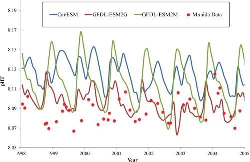
For pH, the present-day output of the six ESMs that incorporate carbonate chemistry was validated against a seven-year pH time series (1998–2005) in subantarctic surface waters (Bates et al. 2014), as in Lenton et al. (2015), who validated ESM projections against Australian coastal pH time series. Comparison of the outputs of the best three ESMs with the time-series data identified that ESM5 provided the best simulation of the magnitude and trend in pH (see Figure 2). In addition, a comparison of modelled Aragonite Saturation Horizon depth with that calculated using a regional algorithm (Bostock et al. 2013), also identified ESM5 as the most appropriate model for the carbonate system in the NZ region (data not shown); consequently, all pH projections are generated using only ESM5.

Figure 2. Comparison of projected surface pH for three ESMs (see legend), with measured pHT (pH total scale at in situ temperature) in subantarctic surface water on the Munida Time Series (Bates et al. 2014) for 1998–2005.

Results and discussion

Physical variables

Sea surface temperature

SST is projected to increase across the SWP by Mid- and End-Century, regardless of emission scenario or ESM (see Figure 3(A)). Ensemble-mean predicted SST increases (ΔSST) by Mid-Century are ∼0.8°C under RCP4.5 and ∼1°C under RCP8.5, and ∼1.1°C under RCP4.5 and ∼2.5°C under RCP8.5 by End-Century. The SST increase by Mid-Century under RCP8.5 is of similar magnitude to that under RCP4.5 by End-Century, highlighting the sensitivity of surface ocean warming to CO₂ emission scenario. Figure 3(A) includes the projected values for each ESM (see Suppl. Table S1), which show a range of 1.6–3.3°C for End-Century under RCP8.5.

Figure 3. A, Projections of mean change in sea surface temperature (ΔSST, °C, ±1 standard deviation) for Mid and End-Century under RCP4.5 and 8.5 (delineated by vertical dashed lines) from the inner ESMs for the SWP (adapted from R16). The numbers indicate the mean for each individual ESM (see Suppl. Table S1). The regional variation of ΔSST for the End-Century under RCP8.5 is shown for B, ESM2 and C, ESM5. The regional boxes are indicated by number, the NZ EEZ boundary by the red line, the white contours the 1000 metre isobath, and the black contours indicate zero change.

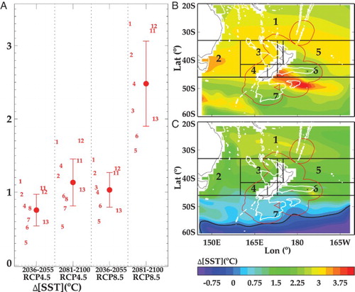
The trend in warming over the twenty-first century is compared to the current mean temperature range using both ESM2 and ESM5 and the RCP4.5 and 8.5 scenarios in Suppl. Figure S1. Although no difference is apparent in projected SST at Mid-Century between emission scenarios, mean SST remains within the present-day range by End-Century under RCP4.5, whereas it is at or above the present-day maximum under RCP8.5. This indicates that marine organisms adapted to the current regional temperature range of these waters may experience thermal stress by 2100.

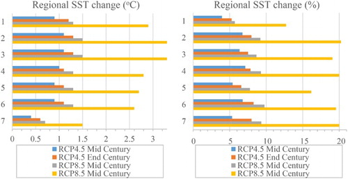
Whereas ESM2 and ESM5 ranked highly in the validation of R16, they generate significantly different ΔSST (2.95°C and 1.6°C, respectively) for the SWP (Figure 3(A)). These projections are comparable to warming estimates for 2100 of 2.67°C (2.04–3.7) for Australian waters (Lenton et al. 2015), and +2.73 (±0.72) °C for the global ocean (Bopp et al. 2013). However, both R16 and Lenton et al. (2015) identify significant regional variability (Figure 3(B,C)). The projected warming with ESM2 is greatest in subantarctic water south of the Chatham Rise, with a tongue of water with a ΔSST of 4°C extending eastwards. ΔSST is also higher in the western Tasman Sea, as reported by Lenton et al. (2015), in association with the southerly extension of the East Australian Current (Ridgway 2007). The ESM2 projection also shows a broad band of ΔSST >3°C extending across the Tasman Sea and into the South Pacific gyre (Figure 3(B)). Although the ESM5 projection shows similar meridional gradients there is less warming overall, with the highest ΔSST (>2.5°C) north and north-east of NZ, and also in the eastern Chatham Rise. ESM5 also shows less warming south of New Zealand in Region 7, and cooling of subpolar surface waters further to the south (Figure 3(C)). The limited warming south of New Zealand is attributed to upwelling-induced cooling associated with seasonal changes in wind-stress curl (Matear et al. 2013). Regional variation in ensemble-average ΔSST from all the inner ESMs shows the largest absolute temperature change in the Tasman Sea under both scenarios and both timeframes, with warming exceeding 3.1°C in regions 2 and 3 by End-Century under RCP8.5 (see Figure 4(A)). Warming is lowest in southern waters with a ΔSST of 1.5°C in region 7. However, when considered as a proportional change in ΔSST, most regions show similar responses, with a maximum of +16% to +20% under RCP8.5 by End Century, except for region 1 which has lower proportional warming (see Figure 4(B)).

Figure 4. Projected ΔSST for all inner ESMs (R16) presented as A, absolute change (Δ,°C), and B, proportional (%) change, for Mid and End-Century for RCP4.5 and 8.5.

Time series observations of SST around NZ are limited, and show conflicting trends, reflecting observation period and region. For example, Uddstrom (2015) found no significant trend in satellite-derived SST during 1993–2012, whereas datasets back to 1960 suggest a significant increase (Mullan et al. 2010). Analysis of a 20-year record of Sea Surface Height has identified an increase in the temperature gradient across the frontal confluence south-east of NZ (Fernandez et al. 2014). A 1°C warming to 800 m was reported in the Tasman Sea for 1996–2002 (Sutton et al. 2005), and recent analysis of SST, XBT and Argo time-series shows warming of the eastern Tasman Sea, on the order of 1.7–3.4°C/century (P. Sutton, pers. comm). The south-west Tasman Sea is a regional hotspot, that is warming faster than the global average, in response to spin-up of the South Pacific gyre (Hill et al. 2008). The current warming rate, of +2.28°C/century to +3.5°C/century (Ridgway 2007; Matear et al. 2013), is similar to the projected rates for some sub-regions of the SWP by 2100 (see Figures 3 and 4). Consequently, the observed changes attributed to warming of the south-west Tasman Sea, which include increases in subtropical water species and oligotrophic conditions, and corresponding declines in primary productivity and temperate water species (Frusher et al. 2014), may provide an analogue for future conditions in NZ surface waters.

Surface mixed layer depth

Changes in SST will impact marine biota directly in terms of physiological processes, and also indirectly through changes in the thermal structure of the upper ocean. For example, a warmer ocean will increase the buoyancy, and decrease the depth of the surface mixed layer (MLD). As the majority of oceanic primary production occurs in the sunlit surface layer, this decrease in MLD may benefit phytoplankton photosynthesis and growth via increased light availability, but conversely an increase in the density gradient at the base of MLD may reduce vertical nutrient supply (Riebesell et al. 2009).

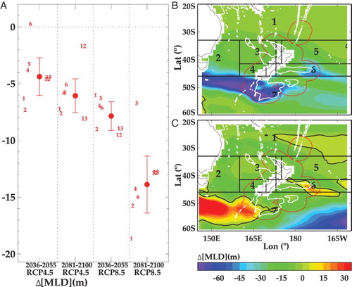
MLD is defined as the depth at which the potential density differs from the surface value by 0.125 kg/m³ (Chiswell et al. 2013). MLD varies seasonally and regionally across the SWP, with a current spring-summer minimum of ∼10 m in subtropical waters to >300 m in winter (Nodder et al. 2016). The MLD is projected to decrease across the SWP, with a mean ΔMLD of −6 m by End-Century under RCP4.5, and −14.5 m under RCP8.5, which is equivalent to a decrease of 15.4% relative to the present-day (see Figure 5(A)). As with SST, the two ESMs show spatial variation in the magnitude and direction of ΔMLD for End-Century under RCP8.5 (see Figure 5(B, C)). ESM2 indicates a significant shallowing of the MLD south-west and south of NZ, and in the eastern Chatham Rise exceeding 45 m, in contrast to ESM5 which shows deepening in both regions (Figure 5(B, C)). However, the two ESMs show general agreement across the rest of the SWP.

Figure 5. A, Projections of the mean change (±1 standard deviation) in the depth of the surface mixed layer (ΔMLD, metres), for Mid and End-Century under RCP4.5 and 8.5 (delineated by vertical dashed lines) from the inner ESMs for the SWP (adapted from R16). The horizontal dashed line indicates zero change in ΔDST and negative values a decrease in MLD, with the numbers indicating the mean for each individual ESM (see Suppl. Table S1). Regional variation in ΔMLD for the End-Century under RCP8.5 is shown for B, ESM2 and C, ESM5. The regional boxes are indicated by number, the white contours show the 1000 metre isobath, and black contours indicate zero change.

Altered light availability in response to a change in MLD may have phenological impacts, affecting the timing and duration of phytoplankton growth and subsequently influencing biotic interactions and the food web. However, the indirect impact of a decrease in MLD may differ between water masses, depending on their nutrient status (Riebesell et al. 2009). An increase in light availability in a shallower surface layer may benefit phytoplankton productivity in colder subantarctic and polar waters that contain sufficient macronutrient concentrations for growth. Conversely, in subtropical waters where the surface layer is characterised by high light and low nutrients, productivity may decline in response to a reduction in vertical nutrient supply. Consequently, warming may have positive effects on food webs in southern NZ surface waters, but negative effects in subtropical waters north of NZ. However, the stimulation by increased light availability may be offset to some extent by a corresponding increase in UV radiation in a shallower surface mixed layer, particularly in polar waters.

Biogeochemical variables

Nutrients

The relative availability of the macronutrients nitrate, phosphate and silicate, and the micronutrient iron, are critical determinants of phytoplankton biomass and community composition. Surface subtropical waters in the SWP are generally characterised by low macronutrient concentrations, and support low phytoplankton biomass. Although subantarctic waters have higher nitrate and phosphate concentrations, phytoplankton growth may be limited by silicate and iron availability (Boyd et al. 1999). However, elevated productivity is associated with the Subtropical Front between the South Island and S.W. Australia, and over the Chatham Rise to the east of NZ, as a result of mixing of these water masses and the resulting increase in micro- and macronutrient availability (Murphy et al. 2001).

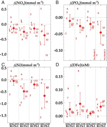
SWP domain-wide mean projections of surface macronutrient concentrations changes show considerable variability (Figure 6), with a non-significant decrease by Mid-Century, and significant decrease by End-Century under both RCP4.5 and 8.5 (see Figure 6(A–D)). End century predictions show an overall decline from present-day concentrations of ∼0.4 (7.5%), 0.05 (9%) and 0.7 (20.3%) mmol m⁻³ for nitrate, phosphate and silicate, respectively under RCP8.5. In contrast to macronutrients, the inner ESM projections indicate an increase in dissolved iron (DFe), of 0.04 mmol m⁻³ by End-Century under RCP8.5, equivalent to 26.9% of present-day mean concentrations (Figure 6(D)).

Figure 6. Projections of the mean change (Δ, ±1 standard deviation) in dissolved surface nutrient concentrations for A, nitrate, B, phosphate, C, silicate, and D, iron for Mid and End-Century under RCP4.5 and 8.5 (delineated by vertical dashed lines) from the inner ESMs for the SWP (adapted from R16). Negative values indicate a decrease in concentration, and positive values an increase in concentration. Vertical dashed lines delineate the projections for Mid- and End-Century under RCP4.5 and 8.5, and the numbers indicate the mean for each ESM (see Suppl. Table S1).

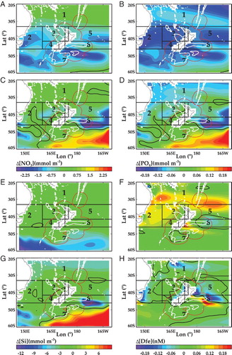
The ESM2 projections for macronutrient concentrations are often relative outliers compared to the other ESMs, showing greater decreases in phosphate and silicate relative to the ESM mean (Figure 6(B,C)). There is also regional variation in the projections of the two ESMs; for example, ESM2 shows a stronger decrease in nitrate and phosphate across much of the NZ EEZ (Figure 7(A, C)). Surface silicate concentrations do not change significantly across much of the NZ EEZ with both ESMs, but a decrease in polar waters occurs south-west of NZ with ESM2 and an increase south-east of NZ with ESM5 (Figure 7(E, G)). Projected changes with ESM2 show a dichotomy in surface DFe between water masses, with a significant increase in subtropical waters and the western Chatham Rise, but negligible change in subantarctic waters (Figure 7(F)). Conversely, ESM5 shows considerable regional variation, with greater increases in DFe in subantarctic waters (Figure 7(H)). Despite regional variations and differences in mean changes, both ESMs confirm the general trends of decreasing macronutrients and increasing DFe. These projections contrast with that of an eddy-resolving model, which predicted increases in nutrient supply to the surface Tasman Sea by Mid-Century in response to increased eddy activity (Matear et al. 2013).

Figure 7. Regional variation of projected change in nutrients for End-Century under RCP8.5, for nitrate using A, ESM2 and C, ESM5; for phosphate using B, ESM2 and D, ESM5; for silicate using E, ESM2 and G, ESM5; and dissolved iron (DFe) using F, ESM2 and H, ESM5. The regional boxes are indicated by number, the NZ EEZ boundary by the red line, the white contour is the 1000 metre isobath and the black contours indicate zero change. The concentration range for each variable is shown by the colour bar beneath each pair of ESM outputs.

These projected changes in nutrient availability may alter regional productivity and food webs. Globally there is evidence that oligotrophic waters are expanding in terms of surface area, in response to warming (Polovina et al. 2011) and, as 50% of NZ waters are, at least seasonally, oligotrophic then future decreases in macronutrient availability may reduce the overall productivity of the EEZ. The decline in phosphate availability in subtropical waters may limit nitrogen fixation, which is a source of new nitrogen that supports productivity in these waters. However, this may be offset by the projected increases in dissolved iron (see Figure 7(E, F)), which is also an important requirement for diazotrophy (Law et al. 2011). The largest projected increase in macronutrients occurs in polar waters south of NZ; however, as these waters have high macronutrients but low DFe, this is unlikely to increase productivity. The Chatham Rise (region 6) is the most productive region in the NZ EEZ, and the projected decline in surface nitrate and phosphate particularly in the east of this region (see Figure 7(A–D), may have ramifications for primary productivity and fisheries (Friedland et al. 2012).

Chlorophyll-a concentration

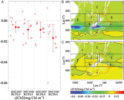
Near-surface Chl-a concentration is an indicator of phytoplankton biomass and a proxy for primary productivity in surface waters (Behrenfeld and Falkowski 1997). Phytoplankton biomass, distribution, functional groups and physiology are influenced by a variety of factors that are sensitive to climate change. Important environmental factors include SST, vertical mixing, mixed layer depth and stratification, all of which influence light and nutrient availability, as well as indirect factors such as grazing and competition for resources. Chl-a projections for the SWP show a minor decrease under RCP4.5 of ∼0.01 mg m⁻³ by 2100 (5% of present-day mean concentration), but a decrease of ∼0.015 mg m⁻³ (7.5% present-day) by End-Century under RCP8.5 (see Figure 8(A)). The ΔChl-a ESM2 projection is low relative to the inner ESM mean, whereas the ESM5 projection is at the upper end of the range (see Figure 8(A)). The regional variation in ΔChl-a is minor across much of the SWP with ESM5, at +0.06 to −0.06 mg m⁻³, whereas ESM2 shows greater decreases by End-Century to −0.5 mg m⁻³ in Subtropical Front waters south of Australia and New Zealand (Figure 8(B)). A minor increase in Chl-a of ∼0.1 mg m⁻³ is projected for the Chatham Rise in region 6 with ESM5 (Figure 8(C)).

Figure 8. A, Projections of mean change (Δ, ±1 standard deviation) in surface Chl-α (mg m⁻³) for Mid and End-Century under RCP4.5 and 8.5 (delineated by vertical dashed lines) from the inner ESMs for the SWP (adapted from R16). Negative values indicate a decrease in concentration, and the horizontal dashed line indicates zero change. The numbers indicate the mean for each individual ESM (see Suppl. Table S1). Regional variation of the projected change in Chl-α for the End-Century under RCP8.5, using B, ESM2 and C, ESM5. The regional boxes are indicated by number, the white contour is the 1000 metre isobath, and the black contours indicate zero change.

Net primary production

A more relevant indicator to marine food webs is the net rate of primary production (NPP), which is the amount of carbon produced per square metre per day integrated over the whole water column. As light, temperature, nutrient concentrations and algal functional group are major factors controlling production (Platt 1986), then NPP is expected to be sensitive to climate change. ESMs generally indicate a reduction in global NPP of 2–13% under high-emission scenarios (Steinacher et al. 2010; Polovina et al. 2011; Bopp et al. 2013), although these show large regional differences. Nevertheless, most ESMs are consistent, in terms of global NPP, in projecting a meridional dichotomy with an increase at high latitudes and a decrease at low latitudes (Pörtner et al. 2014).

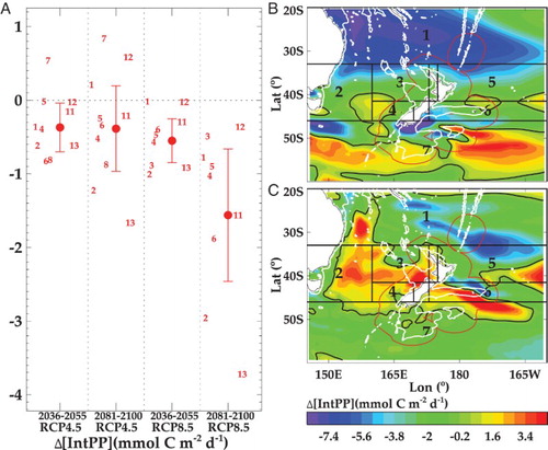
For NZ waters, there is no significant change in NPP by Mid-Century, with decreases of 0.4 and 1.5 mmol C m⁻² d⁻¹ (1.2% and 4.5%, respectively) by End-Century under RCP4.5 and 8.5 (Figure 9(A)). These estimates are considerably lower than the respective global averages, of 3.6% and 8.6% (Bopp et al. 2013), inferring that productivity in the SWP may be relatively less affected by climate change. However, the ESM projections give a broad range of ΔNPP for End-Century under RCP8.5, from 0.3 to 3.7 mmol C m⁻² d⁻¹ (Figure 9(A)), and so there is significant uncertainty. The ESM2 and ESM5 projections both show the largest spatial decline in NPP in subtropical waters north of 40°S (Figure 9(B, C)). This region already experiences very low productivity, with the west end of this meridional band in the South Pacific Gyre recognised as ultra-oligotrophic (Moutin et al. 2012). ESM2 also indicates a decline in NPP south of NZ and Australia, consistent with the Chl-a projection (Figure 9(B)), but increased NPP in subpolar waters south of 48°S. For End-Century under RCP8.5 both ESMs show an increase in NPP in the Tasman Sea, consistent with the 10% increase projected for 2060 by Matear et al. (2013), with this feature extending into subantarctic waters (Figure 9(C)). Whereas NPP in NZ waters may be less affected by climate change than in other regions, the regional trend of a decrease in subtropical waters and increase in temperate and subantarctic waters, is consistent with global projections.

Figure 9. A, Projections of mean change in mean integrated primary production (ΔNPP, ±1 standard deviation) for Mid and End-Century under RCP4.5 and 8.5 (delineated by vertical dashed lines) from the inner ESMs for the SWP (adapted from R16). Negative values indicate a decrease in rate and the horizontal dashed line indicates zero change. The numbers indicate the mean for each ESM (see Suppl. Table S1). Regional variation of the projected change in NPP for the End-Century under RCP8.5, using B, ESM2 and C, ESM5. The regional boxes are indicated by number, the white contour is the 1000 metre isobath and the black contours indicate zero change.

Particle flux

A proportion of the organic matter produced by phytoplankton in the surface ocean sinks through the water column, where it supports the mesopelagic and benthic food web. This particle flux (Exp) is an important vector in determining energy flow through marine ecosystems, and also the amount of carbon sequestered in the deep ocean (Thurber et al. 2014). Elevated phytoplankton biomass is often correlated with higher Exp and greater productivity across trophic levels, although the relationship is complex and often highly variable (Friedland et al. 2012; Nodder et al. 2016). Climate change will likely drive non-uniform variation in ocean conditions, influencing both NPP and the relative proportions that are exported and available to subsurface consumers. Consequently, determining the impact of climate change on particle flux into the ocean interior is important for predicting future ocean carbon uptake and feedbacks, as well as the sustainability of marine ecosystems and fish stocks (Sweetman et al. 2017).

The patterns in detrital flux at the depth of the base of the mixed layer in the two ESMs show good agreement with present-day satellite-based estimates of NPP (http://www.science.oregonstate.edu/ocean.productivity/), and export flux ratio (Law et al. 2016; Pinkerton et al. 2016). Exp is generally higher in the Subtropical Front east and west of NZ (Figure 10(A,D)). ESM2 indicates a general decrease in Exp with time in oligotrophic waters north of NZ and along the Subtropical Front, but an increase in subantarctic waters. Projected decreases are also greater for subtropical waters relative to subantarctic waters with EMS5. These decreases in Exp predominantly reflect the projected decreases in NPP (see Figure 9(B)), as changes in the e-ratio (the export proportion of NPP which exits the base of the mixed layer) are projected to be small (Law et al. 2016; Pinkerton et al. 2016).

Figure 10. A, Present-day mean carbon flux at the base of the surface mixed layer (mg C m⁻² d⁻¹), and projected change (Δ) using ESM2 and RCP8.5 for B, Mid-Century and C, End-Century; D, Present-day mean flux at the base of the surface mixed layer (mg C m⁻² d⁻¹), and projected change (Δ) using ESM5 and RCP8.5 for E, Mid-Century and F, End-Century. Warm colours indicate an increase and cool colours a decrease in flux, with white indicating no change (see legend). The 1000 m isobath is shown by the dashed line.

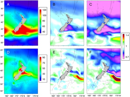
Projected decreases in detrital flux for the NZ region are 4.5% and 12% under RCP4.5 and 8.5, respectively, at End-Century, with the RCP8.5 result outside the range of present-day interannual variability. Projected decreases in global export production under RCP8.5 for End-Century are 7–18% (Bopp et al. 2013), and consequently, reductions in Exp in NZ waters are consistent with global projections. Analysis of the spatial variation in Exp, using the mean of the two ESMs (Table 1), confirms a decrease in most of the SWP sub-regions, with subtropical waters in region 2 experiencing the largest proportional decline, of 11.1% and 23.6% under RCP4.5 and 8.5, respectively, by End-Century. However, the Chatham Rise (region 6), which supports the most productive fishery region in NZ waters (Murphy et al. 2001; SOPI 2015) shows a decline of 12.6% by End-Century, with implications for fish food supply. Application of the Exp projections to assess future suitable habitat for mesopelagic and benthic-feeding fish indicates a decline for all species examined, including commercially exploited species (Law et al. 2016; Pinkerton et al. 2016; Pinkerton 2017). In terms of carbon sequestration, estimates derived from net primary production and an export efficiency of 10% (MacDiarmid et al. 2013), suggest a reduction to ∼0.045 Gt carbon in NZ waters by End-Century under RCP8.5.

Table 1. Projected absolute and proportional (%) change in detrital flux (average value for ESM2 and ESM5) using RCP4.5 and 8.5 for Mid- and End-Century.

Sub-region	Present day (mgC m^−2 d^−1)		% Change
			RCP4.5		RCP8.5
	Mean	Range (2 SD)	Mid Century 2036–2055	End Century 2081–2100	Mid Century 2036–2055	End Century 2081–2100
NZ region	50.2	5.6	−1.3	−4.5	−4.4	−12.0
1	36.4	2.5	−3.1	−11.1	−7.8	−23.6
2	61.5	5.6	−0.5	0.2	−3.3	−5.7
3	51.9	3.0	−0.9	−2.6	−4.7	−8.9
4	63.9	8.9	−1.4	−0.6	−2.3	−3.7
5	50.7	3.7	−2.9	−6.3	−5.4	−15.2
6	79.7	9.8	−3.1	−7.8	−6.7	−12.6
7	54.4	9.4	0.5	0.4	−1.0	−4.7

pH

The transfer of anthropogenic CO₂ into the ocean is altering the oceans carbonate buffering system, lowering pH and carbonate ion availability whilst increasing dissolved CO₂ and bicarbonate (Raven et al. 2005). As these species directly affect chemical reactions and physiological processes then changes in these properties will fundamentally impact both marine biogeochemistry and ecosystems. pH is a measure of hydrogen ion concentration and describes the relative acidity/alkalinity of a solution. Over recent geological time the pH of the ocean has been relatively stable at ∼8.2, but since the late 1870s has declined to 8.1 in response to anthropogenic CO₂ emissions (Raven et al. 2005). As pH is measured on a negative logarithmic scale, this decline of 0.1 is equivalent to an increase in hydrogen ion concentration of ∼30%.

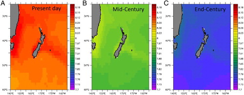
The rate and impacts of ocean acidification in NZ waters are reviewed in Law et al. (2017). The pH of surface water around NZ generally reflects atmospheric CO_2­, as the equilibration time between the surface ocean and atmosphere is on the order of months. There is also no significant upwelling of deep water of lower pH around NZ, and consequentially surface pH is relatively uniform across the region (see Figure 11(A)). The projected surface pH, derived using ESM5, shows a decline in surface pH at both Mid- and End-Century under RCP8.5 across the region (see Figure 11(B, C)), indicating that changes in atmospheric CO₂ concentration override the influence of natural processes on surface water pH. Minor regional variation is evident, with higher pH in northern subtropical waters and the East Australian Current, and lower pH in the south. This meridional gradient of ∼0.03 partially reflects the higher solubility of CO₂, and so lower pH, in colder water. The marginally higher pH in the Subtropical Front over the Chatham Rise may reflect warming (see Figure 3(B)), but also elevated CO₂ uptake by phytoplankton in frontal waters. Conversely, the lowest projected pH of 7.7 occurs in polar waters south of 55°S at End-Century. The projected mean decrease of 0.335 for the NZ region is consistent with projections under RCP8.5 by End-Century for Australian waters (0.304–0.322, Lenton et al. 2015), and the global ocean (Bopp et al. 2013).

Figure 11. The spatial variation in mean surface pH in the SWP for A, the present-day, and projected for B, Mid-Century and C, End-Century, using the ESM5 model under RCP8.5.

Figure 12 illustrates how the surface ocean pH in the NZ region will differ with future emission scenario. The annual sinusoidal pattern in each projection reflects seasonal variation in pH, with a maximum each summer due to phytoplankton uptake of dissolved CO₂, and a minimum in winter due to low phytoplankton productivity and mixing (Currie and Hunter 1999). This seasonality results in a relatively large annual pH range of ∼0.05, which obscures differences in the different RCP projections until ∼2035. However, pH subsequently deviates under the different RCPs, declining to 7.985 by 2050 and 7.95 by 2100 under RCP4.5, equivalent to respective increases of 32% and 42% in hydrogen ion concentration relative to the present-day (see Table 2). The RCP8.5 projection has a steeper pH decline to 7.935 and 7.77 by 2050 and 2100, respectively, with the decline of 0.33 pH units by 2100 (Figure 12), equivalent to an increase in hydrogen ion concentration of 116%.

Figure 12. Projected surface pH for the NZ region under each RCP, with the Mid and End-Century mean pH identified for RCP4.5 (cyan) and RCP8.5 (red). For each RCP, the black line indicates the mean of six ESMs, and the coloured line the EMS5 projection.

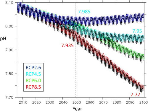
Table 2. Summary table of present-day and projected mean values (Δ = absolute change; % Δ = % change) for the middle and end of the 21^st Century for all variables under RCP4.5 and 8.5 for the SWP region using the inner ESMs (R16).

		Present Day Mean	RCP4.5 Mid-Century			RCP4.5 End-Century			RCP8.5 Mid-Century			RCP8.5 End-Century
Property	Unit		Mean	Δ	% Δ	Mean	Δ	% Δ	Mean	Δ	% Δ	Mean	Δ	% Δ
SST	^oC	15.84	16.6	0.8	4.7	16.9	1.1	6.9	16.8	1	6.6	18.3	2.5	15.8
MLD	m	91	86.5	−4.5	−4.9	85.0	−6	−6.6	83.2	−7.8	−8.6	77.0	−14	−15.4
Nitrate	mmol m^−3	5.31	5.1	−0.2	−3	5.0	−0.28	−5.3	5.1	−0.2	−3.4	4.9	−0.4	−7.5
Phosphate	mmol m^−3	0.5	0.49	−0.01	−2	0.47	−0.03	−5.0	0.48	−0.02	−4.0	0.45	−0.05	−9.0
Silicate	mmol m^−3	3.2	3.1	−0.05	−1.5	2.7	−0.5	−15.6	3.0	−0.2	−6.3	2.55	−0.65	−20.3
Fe	mmol m^−3	0.13	0.16	0.03	19.2	0.17	0.05	34.62	0.14	0.01	7.7	0.16	0.04	26.9
pH		8.11	7.98	−0.12		7.95	−0.16		7.93	−0.18		7.77	−0.33
[H+]	µmol kg^−1	0.008	0.010	0.003	32.1	0.011	0.003	42.2	0.012	0.004	48.3	0.017	0.009	116.3
Chl-a	mg m^−3	0.2	0.19	−0.005	−2.5	0.19	−0.01	−5.0	0.19	−0.01	−5.0	0.185	−0.015	−7.5
NPP	mmol m^−2d^−1	33.52	33.2	−0.35	−1.0	33.1	−0.4	−1.2	33.0	−0.5	−1.5	32.0	−1.5	−4.5
Exp	mg m^−2d^−1	50.2	49	−1.2	−1.3	47.3	−2.8	−4.5	47.5	−2.7	−4.4	43.1	−7.1	−12

The Chatham Rise region has greater interannual pH variation, and a marginally higher projected mean pH, than the NZ mean in 2100, in part due to higher phytoplankton production in the region (Chiswell et al. 2013). Figure 13(A) shows the projected annual mean pH for four ESMs for each RCP to 2100, and to 2050 in Figure 13(B), respectively, for the Chatham Rise region. In both figures the projections are compared to the present-day pH minimum recorded in subantarctic water over a 16-year period at a station on the southern border of region 6 (1998–2014; Bates et al. 2014). This comparison further emphasises the sensitivity of surface pH to future CO₂ emission scenarios. The projected mean pH remains largely within the current pH range under RCP2.6, but falls below the current pH minimum by Mid-Century under all the other RCPs. This ‘point of departure’ (PoD) varies with RCP and model, with the earliest and latest PoD occurring at 2026 and 2034, respectively, under RCP8.5 (see Figure 13(B)). Conversely, the PoD occurs later under the other scenarios, with a PoD of 2031–2040 under RCP4.5 and 6.0, and no PoD before 2100 for two of the four RCP2.6 models (Figure 13(B)).

Figure 13. A, Change in annual pH mean (no seasonality) for the Chatham Rise (region 6) using 4 ESMs (ESM2, ESM5, CANESM2 and GFDL-ESM2M) for each RCP (2.6 dark blue; 4.5 cyan: 6.0 green; 8.5 red) to 2100, compared with the current pH minimum (8.04) measured in subantarctic surface water (horizontal dashed line). B, Expansion of Figure A for the period 2020–2050, with the earliest and latest PoDs projected with RCP8.5 indicated by the red vertical dashed lines.

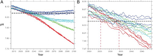
Predicting critical physiological pH thresholds is crucial for assessing the future health of marine ecosystems, and also for marine resources planning and management. Yet this is difficult; despite numerous studies and meta-analysis that have confirmed that ocean acidification has a significant negative effect on marine biota (Kroeker et al. 2013), it is also recognised that there are large differences in thresholds across strains, species and ecosystems. As pH sensitivity differs widely this makes it difficult to predict when deleterious effects may occur. As organisms are assumed to be adapted to present-day conditions, then deviations beyond the current range, as indicated by the PoD, may represent a threshold for ecosystem change. In the case of subantarctic water south of the Chatham Rise, the PoD threshold is projected to occur between 2026 and 2034 (Figure 13(A)).

Current research suggests that ocean acidification may impact productivity and ocean carbon uptake via changes in plankton biodiversity and bacterial processes (Riebesell and Tortell 2011; Burrell et al. 2017). For example, the abundance and distribution of planktonic organisms with carbonate shells may be negatively affected by acidification. The primary calcifying plankton in surface waters in NZ waters are the Foraminifera (Northcote and Neill 2005), Coccolithophores (Chang and Northcote 2016) and Pteropods (Roberts et al. 2014), which have all shown negative responses to lower pH in international studies (Kroecker et al. 2013). Consequently, the projected decline in pH may result in declines in these groups, particularly in subantarctic waters, with implications for associated food webs. Zooplankton and other consumers appear to be less affected, at least directly, by changes in pH and CO₂, although this is based on limited studies. At present, it is too early to determine whether the observed effects of lower pH on behaviour reported for warmer water and reef fish (Munday et al. 2009) will also occur in temperate and subantarctic species in NZ waters.

Conclusions

The surface ocean around NZ will experience warming, with decreases in surface MLD, pH, Chl-a, NPP and particle export by 2100 in response to climate change (see Table 2). Most properties assessed are sensitive to the magnitude of future CO₂ emissions, with the highest emission scenario, RCP8.5, giving the most significant changes, as illustrated by the pH projections (Figures 12 and 13). Whereas the projected differences are generally similar for all RCPs at 2050, they differ between RCP4.5 and 8.5 by End-Century (+1.4°C ΔSST, −0.18 in ΔpH, −2.5% Chl-a, −7.5% export flux). Overall, the projected decreases in NZ waters are generally lower than the respective global thresholds (Bopp et al. 2013), although this is model-dependent, with ΔSST in regions 6 and 7 approaching the global threshold of +3.64°C by 2100 with ESM2 (see Figure 3(B)). Most surface water in the NZ EEZ will be close to the global pH change threshold of −0.36 (Bopp et al. 2013) by 2100, and this rapid decline in surface pH, to levels that are unprecedented on geological timescales (Turley et al. 2006), will exert further pressure on NZ marine ecosystems (reviewed in Law et al. 2017). Indeed, the projected decline in mean pH, to below the current pH minimum by 2040 (Figure 13(A, B)), suggests that organisms with carbonate shells and skeletons may experience corrosive conditions in subantarctic surface waters within one to two decades.

A shift in distribution range in response to warming has been reported for different biotic groups and trophic levels in the global ocean (Poloczanska et al. 2013), and so the projected mean SST increase of 2.5°C by 2100 may result in increasing dominance of warmer-water species in NZ waters. As different trophic levels exhibit different range shifts, interaction and competition between extant and invasive species will result. As identified, comparable increases in SST and resulting ecosystem shifts have already occurred in the south-west Tasman Sea (Cheung et al. 2012; Frusher et al. 2014), and so this region may provide an analogue for future NZ surface waters. However, active relocation by organisms to avoid warmer temperatures may not be straightforward, particularly for calcifying organisms, as southerly migration may increase exposure to lower pH and carbonate undersaturation. This climate-induced narrowing of suitable habitat within the physiological pH and temperature windows may increase the importance of some NZ waters as climate refugia for calcifying groups.

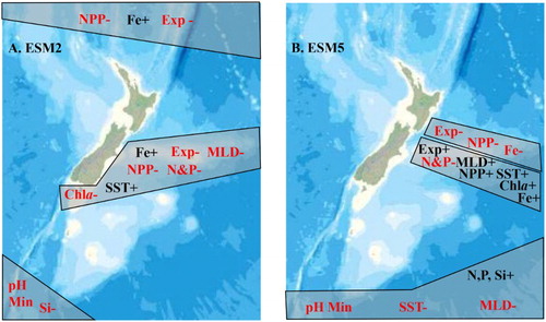
The sub-regions in NZ waters that are potentially more vulnerable to climate change are identified as where the maximum projected regional change occurred for two or more variables (see Figure 14). Although the two ESMs show some contradictory trends, they both identify that the Chatham Rise (region 6) will experience a significant change in a number of parameters by 2100. The region of vulnerability differs between ESMs, extending southward with the Subtropical Front east and south of the South Island in the ESM2 projections (Figure 14(A)), and into subantarctic waters on the northern edge of region 7 with the ESM5 projections (Figure 14(B)). Both ESMs show a decrease in primary production and particle export along the north side of the Chatham Rise, whereas there is an increase to the south with ESM5 that extends into subantarctic waters. In addition, both ESMs indicate that polar waters south of NZ in region 7 are potentially vulnerable to climate change, although there are regional differences, with the most affected waters south of 60°S and south-west of NZ with EMS2, whereas they extend further north to 50°S with ESM5. The ESM2 projections also identify subtropical waters north of 30°S as a potentially vulnerable region, that will experience major decreases in NPP and particle export (see Figure 14(A)).

Figure 14. Regional extremes for climate-sensitive variables in the surface ocean around New Zealand projected for 2080–2100 using A, ESM2 and B, ESM5. The shaded areas represent potentially vulnerable regions, where two or more variables show significant change relative to the NZ mean. The change response is indicated by colour and sign, with a significant decrease indicated in red with a – symbol, and a significant increase in black with a +symbol. Key: SST: Sea Surface Temperature; MLD: Mixed Layer Depth; N&P: Nitrate and Phosphate; Si: Silicate; Fe: Dissolved Iron; Chla: Chlorophyll-a; NPP: Integrated Primary Production; Exp: Particle flux; pH Min: lowest regional pH.

Projections of climate change impacts in NZ waters are currently limited by the spatial resolution of ESMs which, at 1°, are relatively coarse compared to the scale at which biological and ecosystem processes occur. Although ESM2 and 5 generally show consistent trends, they also exhibit regional differences in magnitude and spatial response for some parameters. Although analysis of the reasons for these regional inconsistencies is beyond the scope of this paper, this comparison of ESM2 and 5 outputs demonstrates that there is no single ‘correct’ model. By considering two of the better performing models this comparison illustrates the range of potential outputs accommodated within mean changes over the whole SWP domain, so extending the analysis in R16. The regional inconsistency between two of the best-performing ESMs further emphasises the requirement for a high-resolution regional model of the SWP, to enable downscaling of ESM projections to regional scales and reduce uncertainty.

Nevertheless, the projections emphasise the importance of considering regional variation in climate change response in management and policy decisions. For example, some of the largest projected decreases in macronutrient concentrations occur on the eastern Chatham Rise, a region that supports major fisheries and biodiversity and is a potential location for mineral exploration; consequently, it is critical that climate change is included in assessments of resource use in this region. From a research perspective, organisms and ecosystems in the identified vulnerable regions may experience change over relatively shorter timescales, and so these may be optimal locations for determining ecosystem response and species adaptation capacity. Conversely, regions that are less affected by climate change, such as the central Tasman Sea, may represent potential climate refugia, which should also be considered in assessment of other activities in these regions.

Acknowledgements

Thanks to Steven Stuart for downloading the ESM outputs, Judy Lawrence for assisting with stakeholder engagement and Andrew Tait, Daniel Rutledge and Graham McBride for coordination of the CCII programme. We also thank Scott Nodder, Vonda Cummings, Mary Livingston and Di Tracey for comments on the original report, and Phil Sutton, Jonathan Verlade, Lionel Carter, and two unidentified reviewers for comments on the manuscript. We thank Erika Mackay and Mark Tucker for assistance with figures, the Ocean Biology Processing Group for SeaWiFS data (NASA Goddard Space Flight Center, Ocean Ecology Laboratory, Ocean Biology Processing Group; (2014): Sea-viewing Wide Field-of-view Sensor (SeaWiFS) Ocean Color Data, NASA OB.DAAC http://doi.org/10.5067/ORBVIEW- 2/SEAWIFS OC.2014.0.). Thanks also to the World Climate Research Programme’s Working Group on Coupled Modelling for access to the CMIP5 model output (via https://pcmdi.llnl.gov/projects/cmip5/). WOA2009 data accessed via https://www.nodc.noaa.gov/OC5/WOA09/prwoa09.html.

Disclosure statement

No potential conflict of interest was reported by the authors.

ORCID

Cliff S. Law http://orcid.org/0000-0002-7669-2475

Graham J. Rickard http://orcid.org/0000-0002-0169-4361

Sara E. Mikaloff-Fletcher http://orcid.org/0000-0003-0741-0320

Matt H. Pinkerton http://orcid.org/0000-0001-7948-720X

Erik Behrens http://orcid.org/0000-0002-9713-7227

Steve M. Chiswell http://orcid.org/0000-0002-5957-3706

Kim Currie http://orcid.org/0000-0003-4252-194X

Additional information

Funding

This work was funded by NZ Ministry of Business, Innovation and Employment (MBIE) Contract C01X1225 (CCII), and NIWA Strategic Investment Funding to CAOA1504 (Ocean Climates), and COOF1502 (Oceans: Primary Production).

References

- Aranda M, Christensen A-S. 2009. The New Zealand’s quota management system (QMS) and its complementary mechanisms. In: HaugeKH, WilsonDC, editor. Comparative evaluations of innovative fisheries management. Netherlands: Springer; p. 19–41.
- Bates N, Astor Y, Church M, Currie K, Dore J, Gonzaález-Dávila M, Lorenzoni L, Muller-Karger F, Olafsson J, Santa-Casiano M. 2014. A time-series view of changing ocean chemistry due to ocean uptake of anthropogenic CO2 and ocean acidification. Oceanography. 27(1):126–141. doi: 10.5670/oceanog.2014.16
- Behrenfeld MJ, Falkowski PG. 1997. Photosynthetic rates derived from satellite-based chlorophyll concentration. Limnology and Oceanography. 42:1–20. doi: 10.4319/lo.1997.42.1.0001
- Bopp L, Resplandy L, Orr J, Doney S, Dunne J, Gehlen M, Halloran P, Heinze C, Ilyina T, Séférian R, et al. 2013. Multiple stressors of ocean ecosystems in the 21st century: projections with CMIP5 models. Biogeosciences. 10:6225–6245. doi: 10.5194/bg-10-6225-2013
- Bostock HC, Mikaloff Fletcher SE, Williams MJ. 2013. Estimating carbonate parameters from hydrographic data for the intermediate and deep waters of the Southern Hemisphere oceans. Biogeosciences. 10(10):6199–6213. doi: 10.5194/bg-10-6199-2013
- Boyd PW, Law CS. 2011. An ocean climate change atlas for New Zealand waters. NIWA Information Series. 79:12–13.
- Boyd PW, Law CS, Doney SC. 2011. A climate change Atlas for the Ocean. Oceanography. 24(2):13–16. doi:10.5670/oceanog.2011.42.
- Boyd PW, Lennartz ST, Glover DM, Doney SC. 2014. Biological ramifications of climate-change-mediated oceanic multi-stressors. Nature Climate Change. 5(1):71–79. doi: 10.1038/nclimate2441
- Boyd P, LaRoche J, Gall M, Frew R, McKay RML. 1999. Role of iron, light, and silicate in controlling algal biomass in subantarctic waters SE of New Zealand. Journal of Geophysical Research. 104(C6):13395–13408. doi:10.1029/1999JC900009.
- Burrell TJ, Maas EW, Hulston DA, Law CS. 2017. Variable response to warming and ocean acidification by bacterial processes in different plankton communities. Aquatic Microbial Ecology. 79:49–62. doi:10.3354/ame01819.
- Chang FH, Northcote L. 2016. Species composition of extant coccolithophores including twenty-six new records from the southwest Pacific near New Zealand. Marine Biodiversity Records. 9:75. doi: 10.1186/s41200-016-0077-7
- Cheung WWL, Meeuwig J, Feng M, Harvey ES, Lam V, Langlois TJ, Slawinski D, Sun C, Pauly D. 2012. Climate-change induced tropicalisation of marine communities in Western Australia. Marine and Freshwater Research. 63:415–427. doi:10.1071/MF11205.
- Chiswell SM, Bradford-Grieve J, Hadfield MG, Kennan SC. 2013. Climatology of surface chlorophyll-a, autumn winter and spring blooms in the SWP Ocean. Journal of Geophysical Research: Oceans. 118:1003–1018.
- Currie KI, Hunter KA. 1999. Seasonal variation of surface water CO2 partial pressure in the Southland Current, east of New Zealand. Marine and Freshwater Research. 50(5):375–382. doi: 10.1071/MF98115
- Druel E, Gjerde KM. 2014. Sustaining marine life beyond boundaries: Options for an implementing agreement for marine biodiversity beyond national jurisdiction under the United Nations Convention on the Law of the Sea. Marine Policy. 49:90–97. doi: 10.1016/j.marpol.2013.11.023
- Dunne JP, John JG, Shevliakova E, Stouffer RJ, Krasting JP, Malyshev SL, Milly PCD, Sentman LT, Adcroft AJ, Cooke W, Dunne KA, et al. 2013. GFDLs ESM2 global coupled climate carbon earth system models. Part II: carbon system formulation and baseline simulation characteristics. Journal of Climate. 26:2247–2267. doi: 10.1175/JCLI-D-12-00150.1
- Fernandez D, Bowen M, Carter L. 2014. Intensification and variability of the confluence of subtropical and subantarctic boundary currents east of New Zealand. Journal of Geophysical Research Oceans. 119:1146–1140. doi:10.1002/2013JC009153.
- Friedland KD, Stock C, Drinkwater KF, Link JS, Leaf RT, Shank BV, Rose JM, Pilskaln CH, Fogarty MJ, Stergiou KI. 2012. Pathways between primary production and fisheries yields of Large Marine Ecosystems. PLoS One. 7(1):e28945. doi:10.1371/journal.pone.0028945.
- Frusher SD, Hobday AJ, Jennings SM, Creighton C, D’Silva D, Haward M, Holbrook NJ, Nursey-Bray M, Pecl GT, van Putten EI. 2014. The short history of research in a marine climate change hotspot: from anecdote to adaptation in south-east Australia. Reviews in Fish Biology and Fisheries. 24(2):593–611.
- Hill KL, Rintoul SR, Coleman R, Ridgway KR. 2008. Wind forced low frequency variability of the East Australia Current. Geophysical Research Letters. 35(8). doi:10.1029/2007GL032912.
- Hoegh-Guldberg O, Cai R, Poloczanska ES, Brewer PG, Sundby S, Hilmi K, Fabry VJ, Jung S. 2014. The ocean. In: Barros VR, CB Field, DJ Dokken, MD Mastrandrea, KJ Mach, TE Bilir, M Chatterjee, KL Ebi, YO Estrada, RC Genova, et al., editors. Climate change 2014: impacts, adaptation, and vulnerability. Part B: regional aspects. Contribution of working group ii to the fifth assessment report of the intergovernmental panel on climate change. Cambridge, United Kingdom and New York, NY, USA: Cambridge University Press. p. 1655–1731.
- Hu D, Wu L, Cai W, Gupta AS, Ganachaud A, Qiu B, Gordon AL, Lin X, Chen Z, Hu S, et al. 2015. Pacific western boundary currents and their roles in climate. Nature. 522(7556):299–308. doi: 10.1038/nature14504
- Kroeker KJ, Kordas RL, Crim R, Hendriks IE, Ramajo L, Singh GS, Duarte CM, Gattuso JP. 2013. Impacts of ocean acidification on marine organisms: quantifying sensitivities and interaction with warming. Global Change Biology. 19(6):1884–1896. doi: 10.1111/gcb.12179
- Law CS, Bell JJ, Bostock HC, Cornwall CE, Cummings V, Currie K, Davy SK, Gammon M, Hepburn CD, Hurd CL, et al. 2017. Ocean acidification in New Zealand waters. New Zealand Journal of Marine & Freshwater Research. doi:10.1080/00288330.2017.1374983.
- Law CS, Rickard GJ, Mikaloff-Fletcher SE, Pinkerton MH, Gorman R, Behrens E, Chiswell SM, Bostock HC, Anderson O, Currie K. 2016. The New Zealand EEZ and South West Pacific. Synthesis Report RA2, Marine Case Study. Climate Changes, Impacts and Implications (CCII) for New Zealand to 2100. MBIE contract C01X1225. 41pp.
- Law CS, Ellwood M, Woodward EMS, Marriner A, Bury S, Safi K. 2011. Response of surface nutrient inventories and nitrogen fixation to a tropical cyclone in the South-West Pacific. Limnology Oceanography. 56(4):1372–1385. doi: 10.4319/lo.2011.56.4.1372
- Lenton A, McInnes KL, O’Grady JG. 2015. Marine projections of warming and ocean acidification in the Australasian region. Australian Meteorological and Oceanographic Journal. 65(1):S1–S28. doi: 10.22499/2.6501.012
- Levitus S, Antonov JI, Boyer TP, Baranova OK, Garcia HE, Locarnini RA, Mishonov AV, Reagan JR, Seidov D, Yarosh ES, Zweng MM. 2012. World ocean heat content and thermosteric sea level change (0–2000 m) 1955–2010. Geophysical Research Letters. 39, L10603. doi:10.1029/2012GL051106.
- MacDiarmid AB, Law CS, Pinkerton M, Zeldis J. 2013. New Zealand marine ecosystem services. In: Dymond JR, editor. Ecosystem services in New Zealand – conditions and trends. Lincoln: Manaaki Whenua Press, p. 238–253.
- Matear RJ, Chamberlain MA, Sun C, Feng M. 2013. Climate change projection of the Tasman Sea from an eddy-resolving ocean model. Journal of Geophysical Research Oceans. 118:2961–2976. doi:10.1002/jgrc.20202.
- Moore JK, Lindsay K, Doney SC, Long MC, Misumi K. 2013. Marine ecosystem dynamics and biogeochemical cycling in the community earth system model [CESM1(BGC)]: comparison of the 1990s with the 2090s under the RCP4.5 and RCP8.5 scenarios. Journal of Climate. 26:9291–9312. doi:10.1175/JCLI-D-12-00566.1.
- Moutin T, Van Wambeke F, Prieur L. 2012. Introduction to the biogeochemistry from the oligotrophic to the ultraoligotrophic Mediterranean (BOUM) experiment. Biogeosciences. 9(10):3817–3825. doi: 10.5194/bg-9-3817-2012
- Mullan AB, Stuart SJ, Hadfield MG, Smith MJ. 2010. Report on the Review of NIWA’s ‘Seven-Station’ Temperature Series NIWA Information Series No. 78. 175 pp.
- Munday PL, Dixson DL, Donelson JM, Jones GP, Pratchett MS, Devitsina GV, Døving KB. 2009. Ocean acidification impairs olfactory discrimination and homing ability of a marine fish. Proceedings of the National Academy of Sciences. 106(6):1848–1852. doi: 10.1073/pnas.0809996106
- Murphy RJ, Pinkerton MH, Richardson KM, Bradford-Grieve JM, Boyd PW. 2001. Phytoplankton distributions around New Zealand derived from SeaWiFS remotely-sensed ocean colour data. New Zealand Journal of Marine and Freshwater Research. 35(2):343–362. doi: 10.1080/00288330.2001.9517005
- New Zealand Ministry of Fisheries. 2008. Harvest strategy standard for New Zealand fisheries. 25 p.
- Nodder SD, Chiswell SM, Northcote LC. 2016. Annual cycles of deep-ocean biogeochemical export fluxes in subtropical and subantarctic waters, southwest Pacific Ocean. Journal of Geophysical Research: Oceans. 121:2405–2424. doi:10.1002/2015JC011243.
- Northcote LC, Neil HL. 2005. Seasonal variations in foraminiferal flux in the Southern Ocean, Campbell Plateau, New Zealand. Marine Micropaleontology. 56(3):122–137. doi: 10.1016/j.marmicro.2005.05.001
- Oliver ECJ, Holbrook NJ. 2014. Extending our understanding of South Pacific gyre “spin-up”: modelling the East Australian current in a future climate. Journal of Geophysical Research: Oceans. 119(5):2788–2805.
- Pinkerton MH. 2017. Impacts of climate change on New Zealand fisheries and aquaculture. In: Phillips B.F., Pérez-Ramírez M., editors. The impacts of climate change on fisheries and aquaculture: a global analysis, 1st ed. John Wiley & Sons Ltd.
- Pinkerton MH, Rickard G, Nodder S, McDonald H. 2016. Climate change impacts and implications: net primary production, particulate flux and impacts on fish species in the New Zealand region. NIWA Report.
- Platt T. 1986. Primary production of the ocean water column as a function of surface light intensity: algorithms for remote sensing. Deep-Sea Research (A). 31:1–11.
- Poloczanska ES, Brown CJ, Sydeman WJ, Kiessling W, Schoeman DS, Moore PJ, Brander K, Bruno JF, Buckley LB, Burrows MT, et al. 2013. Global imprint of climate change on marine life. Nature Climate Change. 3:919–925. doi: 10.1038/nclimate1958
- Polovina JJ, Dunne JP, Woodworth PA, Howell EA. 2011. Projected expansion of the Subtropical biome and contraction of the temperate and equatorial upwelling biomes in the North Pacific under global warming. ICES Journal of Marine Science: Journal du Conseil. 986–995. doi: 10.1093/icesjms/fsq198
- Pörtner H-O, Karl D, Boyd PW, Cheung W, Lluch-Cota SE, Nojiri Y, Schmidt DN, Zavialov P. 2014. Ocean systems. In: Field C.B., Barros V.R., Dokken D.J., Mach K.J., Mastrandrea M.D., Bilir T.E., Chatterjee M., Ebi K.L., Estrada Y.O., Genova R.C., et al., editor. Climate change 2014: impacts, adaptation, and vulnerability. Part A: global and sectoral aspects. Contribution of working group II to the fifth assessment report of the intergovernmental panel on climate change. Cambridge: Cambridge University Press; p. 411–484.
- Raven J, Caldeira K, Elderfield H, Hoegh-Guldberg O, Liss P, Riebesell U, Shepherd J, Turley C, Watson A. 2005. Ocean acidification due to increasing atmospheric carbon dioxide. London: The Royal Society.
- Rickard GJ, Behrens E, Chiswell SM. 2016. CMIP5 earth system models with biogeochemistry: an assessment for the southwest Pacific Ocean. Journal of Geophysical Research Oceans. 121:7857–7850. doi:10.1002/2016JC011736.
- Ridgway KR. 2007. Long-term trend and decadal variability of the southward penetration of the East Australian Current. Geophysical Research Letters. 34, L13613. doi:10.1029/2007GL030393.
- Riebesell U, Körtzinger A, Oschlies A. 2009. Sensitivities of marine carbon fluxes to ocean change. Proceedings of the National Academy of Sciences. 106(49):20602–20609. doi: 10.1073/pnas.0813291106
- Riebesell U, Tortell PD. 2011. Effects of ocean acidification on pelagic organisms and ecosystems. In: Gattuso J.-P., Hansson L., editors. Ocean acidification. Oxford: Oxford University Press; p. 99–121.
- Roberts D, Howard WR, Roberts JL, Bray SG, Moy AD, Trull TW, Hopcroft RR. 2014. Diverse trends in shell weight of three Southern Ocean pteropod taxa collected with Polar Frontal Zone sediment traps from 1997 to 2007. Polar Biology. 37(10):1445–1458. doi: 10.1007/s00300-014-1534-6
- Smith RO, Vennell R, Bostock HC, Williams MJ. 2013. Interaction of the subtropical front with topography around southern New Zealand. Deep Sea Research Part I: Oceanographic Research Papers. 76:13–26. doi: 10.1016/j.dsr.2013.02.007
- SOPI. 2015. Situation and Outlook for Primary Industries. 2015. Ministry for Primary Industries. p 72. [accessed 2016 March] http://www.mpi.govt.nz
- Steinacher M, Joos F, Frölicher TL, Bopp L, Cadule P, Cocco V, Doney SC, Gehlen M, Lindsay K, Moore JK, et al. 2010. Projected 21st century decrease in marine productivity: a multi-model analysis. Biogeosciences. 7(3):979–970. doi: 10.5194/bg-7-979-2010
- Sutton PJ, Bowen M, Roemmich D. 2005. Decadal temperature changes in the Tasman Sea. New Zealand Journal of Marine and Freshwater. 39(6):1321–1329. doi: 10.1080/00288330.2005.9517396
- Sweetman AK, Thurber AR, Smith CR, Levin LA, Mora C, Wei CL, Gooday AJ, Jones DO, Rex M, Yasuhara M, et al. 2017. Major impacts of climate change on deep-sea benthic ecosystems. Elementa Science of the Anthropocene. 5:4. doi:10.1525/elementa.203.
- Taylor KE, Stouffer RJ, Meehl GA. 2012. An overview of CMIP5 and the experiment design. Bulletin of the American Meteorological Society. 93:485–498. doi: 10.1175/BAMS-D-11-00094.1
- Thurber AR, Sweetman AK, Narayanaswamy BE, Jones DOB, Ingels J, Hansman RL. 2014. Ecosystem functions and services in the deep sea. Biogeoscience. 11:3941–3963. doi:10.5194/bg-11-3941-2014.
- Turley C, Blackford J, Widdicombe S, Lowe D, Nightingale PD, Rees AP. 2006. Reviewing the impact of increased atmospheric CO2 on oceanic pH and the marine ecosystem. Avoiding Dangerous Climate Change. 8:65–70.
- Uddstrom MJ. 2015. Sea Surface temperature data and analysis for the 2015 synthesis report for the ministry for the environment. NIWA Client report. 26pp.
- van Vuuren DP, Edmonds J, Kainuma M, Riahi K, Thomson A, Hibbard K, Hurtt GC, Kram T, Krey V, Lamarque J-F, et al. 2011. The representative concentration pathways: an overview. Climatic Change. 109:5–31. doi: 10.1007/s10584-011-0148-z
- Weatherdon LV, Magnan AK, Rogers AD, Sumaila UR, Cheung WWL. 2016. Observed and projected impacts of climate change on marine fisheries, aquaculture, coastal tourism, and human health: an update. Frontiers in Marine Science. 3:473. doi:10.3389/fmars.2016.00048.