Anthropogenic increases of catchment nitrogen and phosphorus loads in New Zealand

ABSTRACT

Spatial regression models were used to predict yields (kg ha⁻¹ yr⁻¹) of nitrogen (N) and phosphorus (P) discharged from catchments throughout New Zealand under natural and current conditions. The models were derived using loads (kg yr⁻¹) of TN, NO₃-N, TP and DRP calculated for 592 river water quality monitoring sites. Anthropogenic increases in yields above natural levels were associated with the proportions of catchments occupied by the intensive agricultural land cover and were unevenly distributed across regions. Anthropogenic increases in national loads of TN, NO₃-N, TP and DRP exported to the ocean were 74%, 159%, 48% and 18%, respectively. Increases in loads exported to the ocean varied considerably at smaller scales, with catchments having significant load increases between 4- and 26-fold for N and 6- to 9-fold for P. Predictions of yields and loads reported here have utility in the development of strategies to manage nutrients.

KEYWORDS:

• Nitrogen
• phosphorus
• loads
• yields
• rivers
• intensive agriculture
• anthropogenic increase
• statistical model
• New Zealand

Introduction

Agriculture and other human activities have altered loads of nitrogen (N) and phosphorus (P) lost from land over large regions of Earth (Vitousek et al. 1997; Bennett et al. 2001). Increased N and P loads discharged to aquatic receiving environments are responsible for their degradation from low productivity, or oligotrophic states to eutrophic or hypertrophic states (Rutherford 1984; Smith et al. 2016). Consequently, management of land use to limit the anthropogenic component of catchment nutrient loads is an important issue in many countries (Daily et al. 1997; McDowell et al. 2015). Managing catchment nutrient loads to achieve receiving environment trophic state objectives requires quantification of the anthropogenic component of the total load (i.e. the component in excess of the natural load; Meals 1996; McDowell et al. 2013).

Intensification of land use in New Zealand over the last 20 years, in particular, dairy farming and urbanisation, has resulted in increases in catchment N and P loads (Parliamentary Commissioner for the Environment 2013). The New Zealand National Policy Statement for Freshwater Management (NPS) was promulgated in response to water quality degradation, including increased N and P loads (Ministry for the Environment 2014). The NPS includes requirements for provincial regulatory authorities (regional councils) to set environmental objectives for water bodies and to define management actions to ensure that these are achieved. In order to implement the NPS, regional councils need to determine sustainable catchment N and P loads and to predict the effect of different management strategies on loads (Roygard et al. 2012).

The minimum information that regulatory authorities need to support N and P management strategies are estimates of the anthropogenic contribution to N and P loads across their regions and estimates of the maximum loads that will allow environmental objectives to be achieved (Rouse and Norton 2016). Making these estimates is challenging because of data limitations and the complexity of the processes that mobilise, transport and transform N and P between source areas and receiving environments. Catchment models are frequently used to represent these processes and to make the best use of available data.

There are three main types of catchment nutrient models; mechanistic, budget and statistical models. We used statistical models in lieu of mechanistic or budget models because of the relative ease of set-up and calibration. Statistical models fit observed yields (i.e. load per unit catchment area; kg ha⁻¹ yr⁻¹) to predictors that represent the drivers of nutrient yields. For drivers such as erosion, runoff and leaching, predictor variables may include topographic, climatic geological and land use characteristics (He et al. 2011). Unwin et al. (2010) and Oehler and Elliott (2011) applied machine learning methods to make spatial predictions of N and P concentrations in New Zealand rivers. These studies showed that predictive statistical models can produce accurate predictions of current N and P concentrations at multiple spatial scales, provided there are sufficient input data. The results of the previous statistical models of N and P concentrations suggested that statistical models would also provide accurate predictions of catchment N and P yields and loads.

Achieving good predictive performance from statistical models generally requires the use of multiple predictor variables that are associated with water quality variation, some of which are likely to be correlated. For example, the concentration models of Unwin et al. (2010) and Oehler and Elliott (2011) included predictors that characterised catchment topography, geology and land cover. However, because catchment land use is generally highly correlated with other catchment characteristics, care is required if statistical models are used to predict the effects of anthropogenic pressure such as land use and management on nutrient yields. Some statistical modelling studies have approached the problem of predictor variable intercorrelation by estimating the contribution of anthropogenic pressure to river N and P concentrations over large spatial domains after accounting for the role of other catchment characteristics (e.g. Dodds and Oakes 2004; McDowell et al. 2013). These studies used environmentally defined classes as categorical predictor variables to account for natural variation in factors such as climate, topography and geology. Models were then used to describe the relationships between N and P concentrations and predictor variables representing anthropogenic pressure within sites grouped by the classes. In turn, models were used to estimate the natural state concentrations by setting the anthropogenic pressure predictors to zero (Dodds and Oakes 2004; McDowell et al. 2013). We followed a similar approach; environmental classes were used to account for natural variation in our estimates of natural N and P yields. Evidence for the dependence of N and P yields on anthropogenic pressure in New Zealand includes significantly higher yields from catchments predominantly in dairy, red deer or sheep and beef farms compared to native land use (McDowell and Wilcock 2008).

Our aim was to use statistical models to make spatial predictions of natural and current N and P yields for all rivers in New Zealand. The yield estimates were combined with catchment areas to estimate natural and current N and P loads discharged to the ocean and the anthropogenic increases by differences from natural loads in those loads at catchment, regional and national scales. We operationally defined natural yields and loads as those yields and loads that would occur in the absence of anthropogenic pressure. We used a national dataset of monthly and quarterly observations of N and P concentrations at 592 river water quality monitoring sites across New Zealand to calculate yields of four variables: total N (TN), total P (TP), nitrate N + nitrite N (NO₃-N) and dissolved reactive P (DRP). We quantified the uncertainty associated with our estimates and compared our results to previous estimates of national-scale loads discharged to the ocean that used alternative methods.

Methods

N and P concentration and flow data

We acquired river N and P concentration data from each of New Zealand’s 16 regional councils and unitary authorities and from the National Institute of Water and Atmospheric Research (NIWA). Each council operates a river monitoring network and NIWA operates the National River Water Quality Network (NRWQN). The raw data came from monthly or quarterly samples collected at 780 river monitoring sites distributed across New Zealand, between January 1977 and December 2013 (Figure 1). The aggregated dataset comprised 104,219 water samples in which concentrations of one or more of the variables TN, NO₃-N, TP and DRP were measured.

Figure 1. Spatial distribution of river water quality monitoring sites retained for calculation of nutrient loads. See Table 2 for the number of sites by nutrient variable.

The raw datasets acquired from councils and NIWA varied in structure, reporting conventions, measurement units and laboratory detection and reporting limits. We used a multi-step process described by Larned et al. (2016) to produce an internally consistent dataset. These steps included plotting time-series and using other diagnostic plots to identify and correct data errors such as values being stored in incorrect units and imputing replacement values for censored data (see Larned et al. 2015 for details). For each of the four nutrient variables, two or more measurement methods were reported by the data providers, and we retained data measured using comparable methods. Most councils and the NRWQN use the alkaline persulphate digestion and unfiltered water samples for TN and TP measurements, and molybdenum blue colorimetry with filtered samples for DRP; measurements based on all other methods were omitted. NO₃-N measurements made with ion chromatography, cadmium reduction, azo dye colorimetry or optical sensor were presumed to be comparable (Ormaza-González and Villalba-Flor 1994); measurements based on all other methods were omitted.

For each variable, we excluded monitoring sites for which there were ≤60 sampling dates between 1977 and 2013 and for which the most recent sampling date was before 2011. The 60-sampling date minimum represented a trade-off between the number of sites, which affects spatial coverage and the number of samples, which affect the accuracy of annual load calculations (Snelder et al. 2016). The end date criterion was to ensure that our analysis represented ‘current’ loads. The final N and P dataset consisted of 359,535 concentration measurements at 592 sites (Figure 1).

Load estimates require data describing river flow at the time water samples are taken and either flow time-series or descriptions of flow distributions over the load estimation period. However, only 37% of the sampling dates and 35% of sites in the final dataset were associated with synoptic flow measurements; the other monitoring sites lacked flow recorders. Where flows were not available for the sampling dates, we obtained an estimated mean daily flow from an uncalibrated national hydrological model (TopNet; McMillan et al. 2013; Larned et al. 2015). Flow measurements from recorders were available at all sites with appreciably modified flows (e.g. downstream of hydropower stations). A range of flows were represented at all sites, but most samples were associated with flows close to the median and there was a poorer representation of low and high flows.

To characterise flows at each site over the load estimation period, we used modelled annual flow duration curves (FDCs). FDCs were used in lieu of a flow time-series corresponding to the water samples because we wanted to estimate long-term mean annual loads. The FDC model of Booker and Snelder (2012) provided consistent estimates of the long-term distribution of flows at the monitoring sites.

Load calculation methods

For each monitoring site, we calculated mean annual loads for one or more of the variables TN, TP, NO₃-N and DRP based on two concentration–flow rating curves constructed from the concentration data and the FDCs. The first rating curve was defined by the following model:(1) where are model parameters, is the daily mean flow on days with water samples (m³ s⁻¹), is mean of the natural log of discharge on the sampled days, is time in decimal years, is the mean value of time in decimal years and is the estimated concentration at time i (m³ s⁻¹).

The second rating curve included quadratic terms:(2) The rating curves represented by Equations (1) and (2) are based on the five-parameter (L5) and seven-parameter (L7) regression models of Cohn et al. (1989, 1992). The L5 and L7 models are commonly used when a flow time-series (e.g. mean daily flows) is available for a site (Alexander et al. 2002). Equations (1) and (2) above exclude two terms from the L5 and L7 models that account for seasonality, because our estimates of mean annual loads used annual FDCs. The terms involving time account for temporal trends in concentration, which are commonly observed in New Zealand rivers (Larned et al. 2016).

For each site and variable, the parameters for Equations (1) and (2) were estimated from the sample data by linear regression. Equation (1) was appropriate when a plot of log concentration versus log flow indicated a linear relation. However, nutrient concentration versus flow relations in log–log space are often non-linear (Snelder et al. 2016). In these circumstances, Equation (2) can be a better model as the quadratic term allows the rating curve to accommodate non-linearity (Elliott et al., 2013; Snelder et al., 2016). We determined whether Equation (1) or (2) was most suitable for each site and variable based on model goodness-of-fit and inspection of the regression residuals. We quantified the goodness-of-fit of each rating curve using the mean flow-weighted residual values (ε) from the regression models (Snelder et al. 2016).

We chose the regression models with the lower ε value to define the rating curve, provided the model was statistically significant (p < .05). For cases in which neither model was significant, the rating curve was represented by the mean concentration at all flows. The chosen rating curve for each site and variable (TN, TP, NO₃-N and DRP) combination was then used to predict the concentration for each increment (centile) of flow defined by the FDC for the site. All predictions were made with time set to 31 December 2013. The resulting estimates of were back-transformed by exponentiation to concentration units. Because the models were fitted to log-transformed concentrations, we corrected the retransformation bias using the smearing estimate of Duan (1983):(3) where S is the bias correction factor and are the residuals of the regression model.

We calculated annual loads at each monitoring site by multiplying each flow centile represented by the FDC with the associated concentration estimates and summing these. We expressed these catchment loads as yields (i.e. average load per year per unit upstream catchment area) by dividing the annual load (kg yr⁻¹) by the area of the upstream catchment (ha).(4) where L is the mean annual load expressed as a yield (kg yr⁻¹ ha⁻¹), K is a unit conversion factor (0.316 kg s mg⁻¹ yr⁻¹), A_c is the catchment area (ha), N is the number of centiles represented by the FDC (100), is the estimated concentration at time j (mg m⁻³) and is the flow for each centile of the FDC (m³ s⁻¹).

We assessed the effect of excluding seasonality terms in our rating curve models by calculating loads using the full L5 or L7 models with seasonality terms for the 77 NRWQN sites, for which time-series of mean daily discharge data were available. We fitted the full L5 and L7 models for each site and variable and identified the best-fitting model as described above. We then compared the yields calculated with the full L5 or L7 model and daily discharge times-series to the corresponding yields calculated with the simplified models (Equation (1) or (2)) and FDCs. We summarised the differences between the two sets of loads using three statistics: Nash–Sutcliffe efficiency (NSE; Nash and Sutcliffe 1970), bias and the root-mean-square deviation (RMSD). NSE indicates how closely the observations (taken to be the loads calculated using the L5 and L7 models) coincide with predictions (taken to be the loads calculated using the simplified model). NSE values range from −∞ to 1. An NSE of 1 corresponds to a perfect match between predictions and the observations, values greater than 0 indicates the model has some predictive skill and values greater than 0.5 are commonly considered to indicate good model performance (Moriasi et al. 2007). Bias measures the average tendency of the predicted values to be larger or smaller than the observed values. Optimal bias is zero, positive values indicate underestimation bias and negative values indicate overestimation bias (Piñeiro et al. 2008). RMSD is the mean deviation of predicted values with respect to the observed values and quantifies the characteristic uncertainty of the predictions (Moriasi et al. 2007).

Spatial framework and predictor variables

We used the calculated N and P site yields as response variables in statistical models of natural and current yields. The spatial framework for the models was provided by a digital representation of the national drainage network (Snelder and Biggs 2002). The digital network represents New Zealand’s rivers as 560,000 segments (delineated by upstream and downstream confluences) and their catchments, and is contained in a geographic information system (GIS).

The digital river network has been combined with spatial data layers describing the climate, topography, geology and land cover of New Zealand to produce many catchment characteristics for each network segment (Leathwick et al. 2011; Booker and Snelder 2012). Subsequent modelling has also produced estimates of various hydrological statistics for each segment. We extracted several catchment and hydrological descriptors from the GIS database and used them as predictors in the statistical models of natural and current N and P yields (Table 1). The predictors were chosen based on their association with biological and physical processes that generate, transport and transform N and P loads (Unwin et al. 2010; Booker and Snelder 2012).

Table 1. Catchment characteristics used as predictors in the statistical models of catchment N and P yield.

Predictor	Description	Abbreviation	Unit
Geography and topography	Catchment area	usArea	m^2
	Percentage of upstream catchment occupied by lakes	usLake	%
	Catchment mean elevation	usElev	m ASL
	Catchment mean slope	usSlope	degrees
Climate and hydrology	Catchment annual mean potential evapotranspiration	usPET	mm yr^−1
	Catchment average mean June air temperature	usTmin	degrees C × 10
	Catchment average mean January air temperature	usTmax	degrees C × 10
	Catchment average coefficient of variation of annual rainfall	usRainVar	mm yr^−1
	Catchment average frequency of rainfall >10 mm	usRainDays10	days month^−1
	Catchment average frequency of rainfall > 20 mm	usRainDays20	days month^−1
	Catchment average frequency of rainfall >100 mm	usRainDays100	days month^−1
	Estimated mean flow	MeanFlow	m^3 s^−1
Geology	Catchment average induration or hardness value	usHardness	Ordinal^a
	Catchment average phosphorous	usPhosphorus	Ordinal^a
	Catchment average particle size	usParticleSize	Ordinal^a
	Catchment average calcium	usCalcium	Ordinal^a
Land cover	Proportion of catchment occupied by combination of high-producing exotic grassland, short-rotation cropland, orchard, vineyard and other perennial crops (LCDB3 classes 40, 30, 31, 33)	usIntensiveAg	Proportion
	Proportion of catchment occupied by low-producing grassland (LCDB3 classes 41)	usLowPasture	Proportion
	Proportion of catchment occupied by indigenous forest (LCDB3 class 69)	usNativeForest	Proportion
	Proportion of catchment occupied by indigenous forest (LCDB3 class 71)	usExoticForest
	Proportion of catchment occupied by built-up area,urban parkland, surface mine, dump and transport infrastructure (LCDB3 classes 1,2,5,6)	usUrban	Proportion
	Proportion of catchment occupied by scrub and shrub land cover (LCDB3 classes 50, 51, 52, 54, 55, 56, 58)	usScrub	Proportion
	Proportion of catchment occupied by lake and pond, river and estuarine open water (LCDB3 classes 20, 21, 22)	usWetland	Proportion

^aThe variables usHardness and usParticleSize describe the physical character of the catchment regolith and usPhosphorus and usCalcium characterise its fertility based on values assigned to LRI top-rock categories by Leathwick et al. (2003).

Mean catchment slope, elevation and area in the GIS database were calculated from a digital elevation model (Snelder and Biggs 2002). Estimated mean annual flows were derived using a rainfall-runoff model (Woods et al. 2006). Proportions of catchment land cover were derived from the national land cover database version 3 (LCDB3) which differentiates 33 categories based on the analysis of satellite imagery from 2008 (lris.scinfo.org.nz). Catchment geology was derived from the land resources inventory (LRI; Newsome et al. 2000). Attributes describing the regolith were derived from catchment averages of ordinal values assigned to LRI top-rock categories by Leathwick et al. (2003). Catchment rainfall, potential evapotranspiration (PET) and air temperatures were derived from temperature and rainfall records (Leathwick et al. 2011).

The digital network is the basis of the New Zealand river environment classification (REC; Snelder and Biggs 2002). The REC classifies every segment of the network based on a hierarchy of environmental factors, which are categorical expressions of the catchment characteristics described above (Table 2). The REC classes were used in the statistical models used to predict natural N and P yields to account for natural variation in environmental factors (see Estimating natural catchment yields, below). The second level of the REC is based on a categorical differentiation of catchment climate and topography and is referred to as the Source-of-Flow level. The Source-of-Flow level provides a broad-scale classification comprising 22 classes that discriminate differences in hydrological and water quality characteristics (Snelder and Hughey 2005). Source-of-Flow classes are denoted by the combination of categories that describe the climate and topography of the catchment. For example, most river segments on the south-eastern coast of New Zealand are categorised as Cool-Dry climate and Hill topography and, thus, belong to the CD/H class.

Table 2. Modified river environment classification (REC) classes used by this study, the original Source-of-flow classes (Snelder & Biggs, 2002) that were merged to form each modified class and the number of sites in each class for each nutrient variable.

REC class	Class description	Original classes	Number of monitoring sites
			DRP	NO3-N	TN	TP
CD/H	Cool-dry hill and mountain	CD/H, CD/M	38	38	35	37
CD/L	Cool-dry lowland and lake	CD/L, CD/Lk	78	78	41	77
CW/H	Cool-wet hill	CW/H	129	130	69	126
CW/L	Cool-wet and extremely-wet lowland	CW/L, CX/L	91	91	71	90
CW/Lk	Cool-wet and extremely-wet lake	CW/Lk, CX/Lk	28	28	16	28
CW/M	Cool-wet mountain and glacial-mountain, Cool-extremely-wet mountain and glacial mountains	CW/M, CX/GM, CX/M, CW/GM	19	19	16	17
CX/H	Cool-extremely-wet hill	CX/H	20	21	18	19
WW/L	Warm lowland, hill and lake	WW/L, WX/L, WX/H, WD/Lk, WD/L, WW/Lk, WW/H, WX/Lk	186	185	99	186

Note: See Snelder & Biggs (2002) for a full description of REC classes.

We modified the REC Source-of-Flow levels defined by Snelder and Biggs (2002) by merging classes for which there were few monitoring sites into a smaller number of closely related classes as shown in Table 2. The modification reduced the number of Source-of-Flow classes from 22 to 8. This modification reduced discrimination of environmental variation, but increased the number of sites in each class, which increases statistical power. All 597 monitoring sites were assigned to one of the 8 REC classes (Table 2).

Estimating natural catchment yields

We used analysis of covariance (ANCOVA) to model the natural catchment yields of TN, TP, NO₃-N and DRP. Our method was based on previous applications of ANCOVA to estimate natural N and P concentrations in rivers (Dodds and Oakes 2004; McDowell et al. 2013). In the current study, ANCOVA was used to fit linear relations between the response variables (i.e. catchment yields of TN, NO₃-N, TP and DRP), continuous predictor variables that represented anthropogenic pressure and river size, and REC classes that represented climate and topography. The categorical predictors (REC classes) allowed the relation between yields and the continuous variable to differ by environmental class.

The continuous variable used in the ANCOVA models to represent anthropogenic pressure was the proportion of intensive agricultural land cover in catchments upstream of each segment (usIntensiveAg). Several studies in New Zealand have identified strong associations between water quality and the proportions of catchment land cover representing different types of anthropogenic pressure including urban, pastoral agriculture and exotic forest (Larned et al. 2004; Unwin et al. 2010; Larned et al. 2016). In the present study, usIntensiveAg was calculated by summing the proportions of each catchment into four LCDB3 categories: high-producing exotic grassland, short-rotation cropland, orchard and vineyard and other perennial crops (McDowell et al. 2013; Larned et al. 2016). We considered other descriptors of anthropogenic pressure including the proportion of land occupied by exotic forest and urban development (usExoticForest and usUrban; Table 1). However, to obtain realistic parameter estimates and predictions from linear models, the fitting data need to represent the full range of the explanatory variables. The ranges of usExoticForest and usUrban in the fitting data were truncated compared to their ranges across the whole of New Zealand, and were therefore excluded from the ANCOVA models.

We used mean annual flow, which is independent of both REC classes and usIntensiveAg, as a continuous variable to represent river size (Table 1). River size is associated with N and P yields because N and P concentrations vary in response to an in-stream process that is in turn influenced by size-dependent factors such as residence time and channel hydraulics (Oehler and Elliott 2011).

We transformed the calculated TN, NO₃-N, TP and DRP yields to an approximately normal distribution to improve model performance. We also inspected scatter plots of yield against the continuous predictors for evidence of non-linear relations. Standard forward and backward stepwise linear regression was applied to the saturated ANCOVA models to identify the most parsimonious models. In this procedure, the Akaike information criterion (Akaike 1973) was used to apply a penalised log-likelihood method to evaluate the trade-off between the degrees of freedom and fit of the model as predictor variables were added or removed (Crawley 2002).

Natural N and P yields for each segment in the river network were predicted from the fitted ANCOVA models by setting usIntensiveAg to zero. The predictions were back-transformed by inverting the transformation applied to the response variable, then corrected for retransformation bias using the smearing estimate of Duan (1983). The predictive uncertainties of the ANCOVA models were evaluated by making independent yield predictions for each site using leave-one-out cross-validation, and comparing those predictions to the observations using NSE, bias and RMSD (see section ‘Load calculation methods’).

Mean national-scale natural N and P yields were estimated by averaging predictions over all river segments. Mean natural N and P yields for the 15 jurisdictional regions in New Zealand (Nelson City was merged with the Tasman District) were estimated by averaging predictions over the segments in each region. National and regional natural loads exported to the ocean were calculated by multiplying the estimated natural yields in each terminal segment (i.e. a network segment intersecting the coastline) by the corresponding catchment area, then summing all terminal segment loads nationally and by region.

Spatial modelling of current yield

We used the calculated yields for the 592 sites as training data for random forest (RF) models of current catchment yields of TN, TP, NO₃-N and DRP. All catchment characteristics listed in Table 1 were used as predictor variables used in the RF models. RF is a machine-learning method based on classification and regression trees (Breiman 2001; Cutler et al. 2007). RF models are free from distributional assumptions and automatically fit non-linear relationships and high-order interactions; these models achieve high accuracy by basing predictions on an ensemble of single regression trees (a forest) (Breiman 2001). Detailed descriptions of RF models and their diagnostic tools are described in detail in Breiman (2001) and Cutler et al. (2007).

RF models produce a set of predictions for all cases in the training dataset that is independent of the fitting process and that can be used to evaluate model performance. We quantified performance by comparing the independent predictions with the observations and expressing the degree of agreement using NSE, bias and RMSD (see section ‘Load calculation methods’). We used RF model importance measures to quantify the contribution of each predictor to the model prediction accuracy (Breiman 2001; Cutler et al. 2007). We used partial dependence plots (PDPs) to describe the fitted predictor–response relationships (Cutler et al. 2007).

RF models include any of the original set of predictor variables that are chosen during the model fitting process. However, marginally important predictor variables may be redundant (i.e. their removal does not affect model performance) and their inclusion complicates model interpretation. We used cross-validation and a backward elimination procedure to remove redundant predictors from the models (Svetnik et al. 2004). The procedure recursively removes the least important predictors to identify a ‘reduced’ model whose predictive performance is within one standard error of the best performing model (Breiman et al. 1984).

The fitted spatial models were used to predict current yields in all segments of the digital river network. The predictions were back-transformed by inverting the transformation applied to the response variables and correcting for retransformation bias using the smearing estimate (Equation (3)). Current N and P loads exported to the ocean were estimated for the 15 regions and nationally using the same procedure described above for estimated natural loads.

Increases in catchment yields

Anthropogenic increases in yields were calculated for each segment in the digital river network as the difference between the predicted current and natural yields divided by the natural yield. Anthropogenic increases in N and P loads exported to the ocean were calculated by multiplying the increase in predicted yield for terminal segments by their corresponding catchment areas.

Anthropogenic increases could not always be detected with confidence due to uncertainty in natural and current yield predictions. We assumed that over large areas (i.e. regions or nationally), errors associated with our predictions for individual segments cancelled, leaving only systematic errors (Dymond et al. 2013). Therefore, provided there was no evidence of systematic error (bias) in the models, we summed and averaged all relevant predictions to obtain national and regional estimates of increases in mean yields and loads exported to the ocean. For individual segments, we evaluated confidence associated with estimated yield and load increases using zeta (Z) scores. For each network segment, a Z score was calculated as(5) where Y_c and Y_n are the predicted current and natural yields for the segment and RMSD_c and RMSD_n were calculated using the current and natural yield models, respectively. The calculations were made using transformed values so that Z represented the standard normal deviate. We used an alpha value of 5% and considered that differences in current and natural yields and loads were not significant when −1.96 ≤ Z ≤ 1.96.

Results

Calculated current yields

The L7, L5 and average load calculation methods were the most suitable methods for 74%, 20% and 6% of the site and variable combinations, respectively. Calculated current catchment yields at each monitoring site varied over two orders of magnitude for TN (range: 0.4–73 kg ha⁻¹ yr⁻¹), DRP (range: 0.01 and 5.4 kg ha⁻¹ yr⁻¹) and TP (range: 0.01–8.2 kg ha⁻¹ yr⁻¹). The calculated current yields for NO₃-N varied over three orders of magnitude (range: 0.02–52 kg ha⁻¹ yr⁻¹) (Figure 2). The distributions of the yields were normalised by applying a log₁₀-transformation to TN, TP and DRP yields and a fourth-root transformation to NO₃-N yields. The calculated current yields varied by the REC class, particularly for N (Figure 2). Yields of TN and NO₃-N were the highest in the Lowland topography classes (CD/L, CW/L and WW/L) and the lowest in the Mountain and Hill topography classes (CW/M and CD/H). Yields of TP were the highest in the CW/M class and the lowest in the CD/H class. Patterns in DRP yields were similar to those of N loads, with the highest DRP yields in the Lowland classes (CD/L, CW/L and WW/L) (Figure 2).

Figure 2. Distributions of current catchment N and P yields calculated for all monitoring sites by river environment classification (REC) class. Boxes: third and first quartiles. Solid circle: median. Whiskers: maximum and minimum values. See Table 2 for the number of sites representing each class and nutrient variable.

Comparisons of N and P yields at NRWQN sites calculated using the L5 or L7 models and daily flows versus yields for the same sites calculated using Equations (1) or (2) and FDCs indicated that model simplification had little influence on the calculated yields. NSE values were ≥0.62 and bias was close to 0 indicating that the yields calculated using the FDCs were close to those calculated using daily flows. RMSD values were higher for TP and DRP models, reflecting the poorer performance of these models compared to the TN and NO₃-N models.

Estimated natural catchment yields

The reduced ANCOVA models for TN and NO₃-N explained 57% and 47% of the variation in yields, respectively, and the reduced models for TP and DRP models explained 33% and 26% of the variation in yields, respectively. The correlation between the two covariates in the ANCOVA models, usIntensiveAg and MeanFlow, was small (−0.2). All models included the REC class and both continuous variables (usIntensiveAg and MeanFlow) as model terms (Table 3). In each REC class, TN, TP, NO₃-N and DRP yields increased with increasing proportions of intensive agricultural land cover in the upstream catchment (usIntensiveAg; Table 3). The usIntensiveAg gradient was poorly represented for some REC classes. For example, there were no sites in the CW/M and CX/H classes with usIntensiveAg >56% cover, and 75% of the sites in the CD/L class had usIntensiveAg >64% cover. The yields of each nutrient variable increased with the mean flow in most REC classes (Table 4).

Table 3. Coefficients for terms retained in the reduced ANCOVA models of nutrient yield.

Class	TN	NO3-N	TP	DRP
CD/H	−0.15	0.71	−1.1	−1.76
CD/L	0.1	0.98	−0.97	−1.44
CW/H	0.36	1.03	−0.6	−1.15
CW/L	0.57	1.23	−0.62	−1.21
CW/Lk	0.03	0.67	−0.99	−1.22
CW/M	0.21	0.83	−0.3	−1.2
CX/H	0.41	0.93	−0.38	−0.94
WW/L	0.68	1.15	−0.57	−1.08
usIntensiveAg	0.86	0.63	0.43	0.44
log10(MeanFlow)	0.07	0.06	0.18	0.03
CD/L:usIntensiveAg	0.08	0.12
CW/H:usIntensiveAg	−0.18	0.25
CW/L:usIntensiveAg	−0.37	−0.21
CW/Lk:usIntensiveAg	0.55	1.03
CW/M:usIntensiveAg	−0.28	0
CX/H:usIntensiveAg	0.28	0.8
WW/L:usIntensiveAg	−0.42	0.04

Note: The response units for TN, TP and DRP are log₁₀ kg ha⁻¹ yr⁻¹, and for NO₃-N are kg^0.25 ha⁻¹ yr⁻¹.

Table 4. Performance of the ANCOVA models of natural yields and RF models of current yields.

Model	Nutrient	NSE	Bias	RMSD
ANCOVA
(Natural yields)	DRP	0.23	0.0000	0.38
	NO3-N	0.43	−0.0005	0.29
	TN	0.52	0.0001	0.26
	TP	0.31	0.0002	0.37
RF
(Current yields)	DRP	0.50	−0.005	0.30
	NO3-N	0.58	−0.009	0.25
	TN	0.59	−0.005	0.24
	TP	0.50	0.004	0.32

Note: The performance statistics were computed with the transformed yields and therefore units of bias and RMSD are log₁₀ kg ha⁻¹ yr⁻¹, for TN, TP and DRP and kg^0.25 ha⁻¹ yr⁻¹ for NO₃-N.

The reduced TN and NO₃-N models included interaction terms between REC class and usIntensiveAg. The reduced TP and DRP models had no interaction terms (Table 3).

The reduced ANCOVA models for TP, NO₃-N and DRP yield had NSE values <0.5 (Table 4), indicating the predictions had low accuracy (Moriasi et al. 2007). All four models had low bias. RMSD values were higher for the TP and DRP models than for the TN and NO₃-N models, reflecting the poorer performance of the TP and DRP models (Table 4).

The coefficients for the REC classes in the ANCOVA models (Table 3) indicate the natural variation in N and P yields, controlling for the effect of anthropogenic pressure (i.e. usInstensiveAg) and mean annual flow (MeanFlow). The maps of predicted natural yields (Figure 3) not only reflect the REC class coefficients but also include the effect of mean annual flow. Natural TP yields were the greatest in rivers in the CX/H, CW/M classes; these classes occur on the west coast of the South Island, and in some mountain ranges in the North Island (Figure 3). Natural TP yields were the lowest in the Central Otago and central Canterbury and Southland regions, where most rivers are in the CD/H, CD/L and CW/Lk classes. Natural TN yields were the greatest in the low-elevation areas of the North Island, where most rivers are in the WW/L class, and in the low-elevation areas of the West Coast Region, which are dominated by rivers in the CW/L class (Figure 3). Natural TN yields were lowest in the higher and dryer areas of the South Island that are dominated by rivers in the CD/H, CW/Lk, CD/L and CW/M classes (Figure 3).

Figure 3. Spatial distribution of predicted natural yields of TN, NO₃-N, TP and DRP derived from the ANCOVA models All 560,000 segments making up the digital river network are shown. Colour scales differ by nutrient variable and divide the range in predicted values into quantiles.

Natural DRP yields were the greatest in rivers draining the hill catchments on the West Coast region (CX/H class) and low-elevation rivers of the North Island (predominantly WW/L class; Figure 3). Natural DRP yields were the lowest on the eastern and southern lowland areas of the South Island, in rivers in the CD/H and CD/L classes (Figure 3). Natural NO₃-N yields were the greatest in low-elevation areas of the North Island (WW/L class) and in the wetter lowland areas of the South Island including the West Coast and parts of Southland, which are dominated by rivers in the CW/L class (Figure 3). Natural NO₃-N yields were the lowest in the dry south-eastern portion of the South Island, the Southern Alps and the volcanic plateau in the North Island.

The national natural loads of TN and NO₃-N discharged to the ocean were 108 and 44 Gg yr⁻¹, respectively. The national natural loads of TP and DRP discharged to the ocean were 21 and 3 Gg yr⁻¹, respectively (Table 5).

Table 5. Predicted natural and current loads and anthropogenic increases for regional and national loads exported to the ocean for the four nutrient variables.

Region	TN	TP	NO3-N	DRP
Northland	6, 10.6, 77	0.7, 0.8, 8	2.4, 4.6, 89	0.2, 0.2, 29
Auckland	1.7, 3.6, 107	0.2, 0.2, 46	0.7, 1.9, 174	0.1, 0.1, 18
Waikato	14.9, 27.1, 82	2.5, 2.1, −15	6.5, 20, 210	0.3, 0.5, 42
Bay of Plenty	5.9, 8.2, 40	1.1, 1.2, 12	2.4, 5, 108	0.2, 0.3, 85
Gisborne	3.2, 4.3, 36	0.6, 1.2, 104	1.2, 3.5, 188	0.1, 0.1, 24
Taranaki	3.6, 9.3, 156	0.5, 1, 105	1.8, 5.9, 226	0.1, 0.2, 71
Manuwatu-Wanganui	10.4, 21.1, 102	1.9, 3.6, 86	6.3, 12.1, 93	0.2, 0.4, 50
Hawkes Bay	6, 11.5, 91	1.1, 3, 162	2.7, 8.7, 224	0.2, 0.3, 94
Wellington	3.7, 6.6, 76	0.6, 1, 79	2.3, 3.8, 67	0.1, 0.1, 45
Tasman	2.3, 3.2, 38	0.5, 0.6, 30	1, 1.8, 83	0.1, 0.1, −8
Marlborough	2.7, 3.5, 28	0.5, 0.8, 56	1.3, 2.1, 71	0.1, 0.1, −15
West Coast	13.1, 15.3, 17	4, 4.6, 13	4.7, 6.4, 34	0.4, 0.4, −12
Canterbury	15.3, 28.7, 87	3.7, 4.5, 22	5.4, 19.2, 257	0.5, 0.3, −29
Otago	7.9, 13.8, 74	1.3, 4.4, 228	2, 7, 257	0.3, 0.3, 15
Southland	10.6, 20.4, 92	1.6, 1.8, 10	3.6, 12.5, 244	0.3, 0.3, −14
Total	108, 187, 74	21, 31, 48	44, 114, 159	3, 4, 18

Note: In each table cell, the first two values are the natural and current loads (Gg yr⁻¹) and the third value is the anthropogenic increase (values represent the percentage increase in natural loads).

Spatial modelling of current catchment yields

All four RF models had NSE values ≥0.5 and low bias (Table 4), indicating good model performance (Moriasi et al. 2007). NSE values were higher, and RMSD values were lower, for TP and DRP, indicating poorer model performance compared with the TN and NO₃-N models (Table 4).

The reduced RF models of current TN, NO₃-N and DRP yields included all 23 predictors and the reduced model of current TP yield included 12 predictors. The overall highest ranked predictors (i.e. across all four nutrient variables) were usIntensiveAg, usTmin and usElev (Figure 4). For individual variables, the most important predictors were usIntensiveAg for the NO₃-N and TN models, usRainDays20 for the TP model and usTmin for the DRP model; usIntensiveAg was the 3rd and 14th most important predictor for the TP and DRP models, respectively.

Figure 4. Partial dependence plots for the 12 predictors that were ranked in the 6 most important predictor variables for at least one of the current nutrient yield models, except for usRainDays10, which was similar to usRainDays20 (see Table 1 for explanation of predictors). Standardised values of the marginal responses are on the Y-axes. For each modelled variable, the original marginal responses over all nine predictors were standardised to have a range between zero and one. The amplitude of each plot (i.e. the range of the marginal response) is related to variable importance (amplitude is large when the variable has high importance). The ticks on the top of the x-axes indicate deciles of the distribution of the predictors represented in the monitoring site dataset.

Partial dependence plots for highest ranked predictors for the RF models indicated that there were positive relationships between current yields of all four nutrients and intensive agriculture land cover (usIntensiveAg), the frequency of heavy rainfall (usRainDays10, usRainDays20), catchment area (usArea) and mean flow (MeanFlow) (Figure 4). Current yields of all four nutrients decreased with increasing values of native forest cover, low-producing grassland cover and regolith particle size and hardness (usNativeForest, usLowPasture and usHardness). TN, NO₃-N and DRP yields decreased and TP yields increased with increasing catchment slope (usSlope). There were complex relationships between loads and mean June air temperature (usTmin) particularly for NO₃-N and DRP, which had maximum values at approximately 3°C (Figure 4).

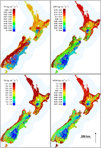
Geographic patterns of predicted current yields differed among the nutrient variables (Figure 5). Current TN and NO₃-N yields are the greatest in lowland areas of the Southland, Canterbury, Taranaki, Hawkes Bay, Manawatu-Whanganui and Bay of Plenty regions, in the Waikato region downstream of Lake Taupo, and in parts of Auckland and Northland (Figure 5). Current yields of TN and NO₃-N were the lowest in upland catchments of the North and South Islands, and in lowland areas dominated by indigenous forests, such as Stewart Island and Fiordland (Figure 5).

Figure 5. Spatial distribution of predicted current nutrient yields derived from the random forest models. All 560,000 segments making up the digital river network are shown. Colour scales differ by nutrient and divide the range in predicted values into quantiles.

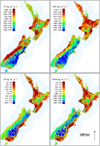
Current TP yields were the highest in rivers draining high rainfall and steep catchments in the West Coast, and in the Taranaki, Manawatu-Whanganui and Gisborne regions, and the lowest in eastern areas of the South Island and the inter-montane basins of Otago and Canterbury. Current DRP yields were the highest in catchments draining lowland areas of the West Coast, the Taranaki regions and coastal catchments of the Hawkes Bay, Manawatu-Whanganui, Bay of Plenty regions and the Waikato region downstream of Lake Taupo, and the lowest in eastern catchments of the South Island (Figure 5).

The national current loads of TN and NO₃-N discharged to the ocean were 187 and 114 Gg yr⁻¹, respectively. The national current loads of TP and DRP discharged to the ocean were 31 and 4 Gg yr⁻¹, respectively (Table 5).

Anthropogenic increases in loads and yields

The predicted anthropogenic increase in the national load exported to the ocean was the largest for NO₃-N (161%) followed by TN (73%), TP (48%) and DRP (18%) (Table 5). Increases in loads exported to the ocean varied widely across regions (Table 5). Increases in NO₃-N loads exported to the ocean exceeded the national average in the Otago, Canterbury, Southland, Hawkes Bay, Taranaki, Gisborne, Waikato and Auckland regions. Increases in TN loads exported to the ocean exceeded the national average in the Manawatu-Wanganui, Southland, Canterbury, Otago, Taranaki and Hawkes Bay regions. Increases in TP exceeded the national average in the Otago, Marlborough, Wellington, Hawkes Bay, Taranaki and Gisborne regions. Increases in DRP exported to the ocean exceeded the national average in the Northland, Waikato, Bay of Plenty, Taranaki, Manawatu-Wanganui, Hawkes Bay and the Wellington regions. For six regions, the anthropogenic changes in TP or DRP loads exported to the ocean were negative, indicating that predicted current loads were lower than natural loads (Table 5).

Increases in TN and NO₃-N yields for individual segments of the river network were not significant unless they were larger than a factor of 6.4 and 4.0, respectively (Figure 6). NO₃-N and TN increases were significant for 22% and 3% of all segments, respectively. Segments with significant NO₃-N increases were distributed over both the South and North Islands. Large contiguous areas with significant increases in NO₃-N yield were associated with high values of usIntensiveAg in the Southland, Otago Canterbury, Marlborough, Wellington, Taranaki, the Manawatu-Whanganui, Hawkes Bay Waikato and Northland regions (Figure 6).

Figure 6. Spatial distribution of the estimated increase in nutrient yields (as a factor of the predicted natural yield) for each network segment. Increases are only shown for network segments with significant differences (−1.96 ≤ Z ≤ 1.96) between natural and current yields. Colour scales differ by nutrient and divide the range in predicted values into quantiles.

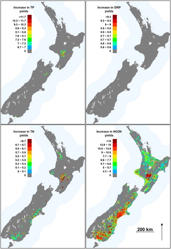
Individual terminal segments (representing whole catchments) with significant NO₃-N load increases were distributed over all 15 regions; however, some regions were disproportionately represented. Of the 1700 terminal segments with significant increases in NO₃-N loads, 26% were in Canterbury, 14% in Auckland and Otago, and 11%, 8%, 7% and 6% were in Taranaki, Bay of Plenty, Northland, Waikato and Southland, respectively. All other regions made less than a 4% contribution to the national set of terminal segments with detectable NO₃-N load increases. Terminal segments of large rivers (catchment area >500 km²) with detectable NO₃-N load increases included the Waiau River in Southland (10-fold increase), the Opihi, Orari, Waihao, Rangitata and Selwyn Rivers in Canterbury (between 4- and 6-fold increases), the Tukituki River in Hawkes Bay (5-fold increase), the Turakina in Manawatu (5-fold increase) and the Awatere in Marlborough (4-fold increase).

Only 350 individual terminal segments had significant TN yield increases and these were confined to the Canterbury and Southland regions. Most of these (98%) represented catchments of less than 200 km² in area. Factorial increases in TP and DRP yields that were significant were twice as high as for TN and NO₃-N, reflecting the larger uncertainties associated with the P models (Figure 6). Significant increases in DRP were negligible and TP increases were only detectable for 2% of network segments (Figure 6). Only 30 terminal segments had significant TP load increases and these were distributed over five regions Southland, Canterbury, Otago Tasman and Taranaki. Increases in TP loads from these catchments ranged between 6- and 9-fold. All terminal segments with significant TP load increases represented small catchments.

Discussion

Predicted N and P yields, loads and anthropogenic increases

Water quality and eutrophication are significant issues in New Zealand (Parliamentary Commissioner for the Environment 2013). Given the importance of agriculture to the New Zealand economy and the regulatory requirements to determine sustainable N and P loads, it is important to increase our understanding of the causes of variation in nutrient yields and to improve the accuracy of predictions of nutrient losses from land. Our predictions of natural and current yields of TN, TP, NO₃-N and DRP indicate that the current yield of each nutrient is elevated above the natural state over large parts of New Zealand. Our observations that yields of each nutrient variable were positively associated with high-intensity agriculture and varied with climate conditions and other environmental drivers are consistent with previous studies of concentrations of the same nutrient variables (Larned et al. 2004; Unwin et al. 2010; Larned et al. 2016).

Our operational definition of natural yields does not account for differences in nutrient attenuation in the pre-agricultural New Zealand landscape compared with the modern landscape. Attenuation may have been higher prior to agricultural development due to greater retention of water in catchment soils and greater connectivity of hillslopes with wetlands and floodplains (Howarth et al. 1996; Mitsch et al. 2005). Our natural yield models do not represent these attenuation mechanisms and assume that anthropogenic increases are only driven by changes in land use. It is therefore likely that our predictions represent upper and lower bounds for the actual natural nutrient yields and anthropogenic increases, respectively.

Spatially averaged N and P yields, and anthropogenic increases in those yields varied with spatial scale. For example, significant increases in NO₃-N exported to the ocean varied from 0.3- to 2.6-fold among regions and from 4- to 90-fold between individual river segments. We do not expect that spatial patterns in nutrient loading will be consistent with spatial patterns in ecosystem responses (e.g. primary production) because of spatial variation in ecosystem sensitivity to nutrient enrichment. The variability in ecological responses to external N and P loading to rivers, lakes and estuaries has been demonstrated in multiple regional studies (e.g. Valiela et al. 1997; Snelder et al. 2004; McLaughlin et al. 2014).

Prediction uncertainties

Loads estimated from N and P concentrations in monthly grab samples are invariably characterised by high uncertainty (Defew et al. 2013; Snelder et al. 2016). In addition, our load calculations used FDCs in lieu of river flow time-series and ignored seasonality. However, these two simplifications had minimal effects on the calculated loads compared to calculations using the L5 or L7 methods and daily flows. Therefore, uncertainties associated with the calculated site loads are irreducible unless the frequency of water sampling for N and P measurement is increased (Snelder et al. 2016). The uncertainties associated with load calculations contributed to subsequent uncertainty in the spatial predictions of yields. However, our spatial models had low bias (Table 4), and it is likely that prediction errors for individual segments cancelled when they were aggregated over catchments, regions and nationally.

Our natural yield models only included anthropogenic pressure represented by intensive agriculture and did not account for urbanisation, point sources or other pressures. The influence of urban areas could not be represented in the natural yield model due to the small number of sites with urban land cover in the fitting data. Urban areas were represented in the current yield models but point sources were not included in either the current or natural yield models. Elliott et al. (2005) reported that point sources contribute only 3.2% and 1.8% of TN and TP loads exported from New Zealand catchments to the ocean. Therefore, we assume that point sources make minimal contributions to regional and national loads and the effects of their exclusion on the yield–environment relationships in our models were also minimal. Furthermore, given the small contribution of point sources to loads nationally, it is unlikely that their exclusion increased the uncertainty of our statistical models. Similarly, given the small extent of urban areas, we assume that their exclusion from the natural yields model had little effect on the uncertainty of our national and regional estimates.

The TP and DRP load models had lower performance (i.e. lower NSE values) than the TN and NO₃-N load models (Tables 4, 6), which is consistent with load and concentration models in other New Zealand studies (Alexander et al. 2002; Unwin et al. 2010; Oehler and Elliott 2011). There are two possible explanations for the relatively poor performance of the P models. First, P load calculations for individual monitoring sites are often associated with higher uncertainty than N loads (e.g. Table 3). The performance of the P models was therefore limited to a greater extent by uncertainty of the modelled response (yield) than the N models. Second, the redox states of soils affect P retention and transport (Hively et al. 2005; Dymond et al. 2013), and soil redox state may be poorly represented by our environmental predictors. Inclusion of soil anion storage capacity, as used in localised and national-scale estimates of DRP leaching, could increase the accuracy of our catchment P yield models (McDowell and Condron 2004; Dymond et al. 2013).

Comparisons with other nutrient yield and load estimates

Our predictions of national and regional current nutrient loads exported to the ocean can be compared to estimates made for the same areas using different methods. Current national loads of TN and TP exported to the ocean were estimated by Elliott et al. (2005) using SPARROW models, fitted to data from the 77 NRWQN sites. Elliott et al. (2005) estimated a national TN load exported to the ocean of 167 Gg yr⁻¹, which is close to our prediction of 187 Gg yr⁻¹ (Table 5). Elliott et al. (2005) estimated a national TP load to the ocean of 63 Gg yr⁻¹, considerably higher than our estimate of 30 Gg yr⁻¹ (Table 5). A potential reason for this difference is the uncertainty associated with the calculated yields, which are generally higher for TP than the other nutrient variables (Snelder et al. 2016). It is also possible that TP loads were overestimated by Elliott et al. (2005). Evidence for this is that our results indicate that river size (as indicated by mean annual flow) influences TP loads to a greater degree than the other nutrient variables (Figure 4, Table 4). Because Elliott et al. (2005) calibrated their model using loads estimated for NRWQN sites, which are strongly biased to large rivers, their model may not adequately represent the reduction in TP loads with decreasing river size.

Geographic patterns in our predictions of current NO₃-N and DRP yields are not comparable to the subsurface losses (i.e. leaching losses) of NO₃-N and DRP predicted by Dymond et al. (2013) because we predicted ‘environmental loads’ (i.e. loads at points in the drainage network) whereas Dymond et al. (2013) predicted ‘source loads’ (i.e. loads at sources such as land surfaces). Source loads and yields have the same units as environmental loads and yields, but environment loads are generally attenuated by biogeochemical processes in the drainage system (e.g. denitrification) and may be lagged due to long travel times and transient storage in hydrological networks.

The analysis by Dymond et al. (2013) was based on budget models with a spatial resolution of 100 m², which is comparable to the grain of our network yield predictions. Dymond et al. (2013) predicted the greatest NO₃-N source yields ( > 30 kg ha⁻¹ yr⁻¹) in parts of Northland, Waikato, Bay of Plenty, Taranaki, eastern Manawatu, South Canterbury and Southland and some small patches on the West Coast. The same locations had the greatest current NO₃-N yields in our study. The mean NO₃-N source yields in the Dymond et al. (2013) study were, on average, twice as high as our calculated current yields, which suggests that 50% of the NO₃-N lost from land as source loads is attenuated before reaching downstream monitoring sites. Dymond et al. (2013) predicted subsurface concentrations of DRP (i.e. leachate), rather than source yields, and did not include losses from surface processes which precludes comparisons with our predictions of DRP yields.

Previous estimates of national and regional-scale N and P loads exported from New Zealand catchments to the ocean were made using budget models (Parfitt et al. 2008, 2012), but those estimates are not comparable to ours for two reasons. First, soluble N in the Parfitt et al. (2012) study consisted of NO₃-N, plus other forms of dissolved inorganic and organic N, and this mixture is not comparable with our estimates of NO₃-N loads. Second, Parfitt et al. (2008, 2012) included erosion, but not biogeochemical processes in their TN and TP budgets.

Use of estimated N and P yields

The development of strategies to manage diffuse-source contaminants generally involves five analytical steps that are undertaken at catchment scales (USEPA 2007). First, the contaminants of concern are selected. In New Zealand, consideration of nutrients is mandated by the NPS, which requires that numeric objectives for trophic state are set for lakes (chlorophyll biomass) and rivers (periphyton biomass) and that impacts of land-based activities on coastal environments are taken into account. Second, the assimilative capacity of waterbodies is estimated. Within a catchment, there is generally a range of waterbodies with differing assimilative capacities. In the New Zealand context, the assimilative capacity of a waterbody for nutrients is the maximum nutrient load that will allow the designated trophic state objective for the waterbody to be achieved (Snelder et al. 2004). Third, the current loads from all catchment sources are estimated. Fourth, an analysis of how current contaminant loads can be reduced to levels that will allow objectives to be achieved is undertaken. Fifth, allowable contaminant loads (which may incorporate margins of safety) are allocated among the different catchment sources.

The results of our study can assist with the third step in the process set out above by providing predictions of current and natural yields for any catchment receiving environment. Estimates of loads discharging to lakes and estuaries can be obtained by adding the contributions from all influent tributaries. The fourth step is generally carried out using catchment models such as SPARROW (Elliott et al., 2005) and CLUES (Elliott et al. 2016), and our predicted yields may be used as calibration data and for testing catchment model predictions.

Acknowledgements

We thank the regional and district council staff who provided water quality data and details about monitoring programmes and methods. We thank Leigh Stevens (Wriggle – Coastal Management) for early discussions and Julian Sykes and Hilary McMillan (NIWA) for assistance with GIS analyses and TopNet output for flow estimates, respectively. We also thank reviews by three anonymous reviewers and NZJMFR editors whose comments improved this article.

Disclosure statement

No potential conflict of interest was reported by the authors.

Additional information

Funding

This work was funded by the Ministry of Business, Innovation and Employment, contract numbers: C01X1318 – Ngā Kete o Te Wānanga: Mātauranga, and C10X1507 – Our Land and Water National Science Challenge.

References

- Akaike H. 1973. Information theory and an extension of the maximum likelihood principle. In: Petrov BN, Csaki F, editor. Akademiai kiado. Budapest: Springer Verlag; p. 267–281.
- Alexander RB, Elliott AH, Shankar U, McBride GB. 2002. Estimating the sources and transport of nutrients in the Waikato river basin, New Zealand. Water Resources Research. 38:1268–1291. doi: 10.1029/2001WR000878
- Bennett EM, Carpenter SR, Caraco NF. 2001. Human impact on erodable phosphorus and eutrophication: a global perspective. BioScience. 51:227–234. doi: 10.1641/0006-3568(2001)051[0227:HIOEPA]2.0.CO;2
- Booker DJ, Snelder TH. 2012. Comparing methods for estimating flow duration curves at ungauged sites. Journal of Hydrology. 434–435:78–94. doi: 10.1016/j.jhydrol.2012.02.031
- Breiman L. 2001. Random forests. Machine Learning. 45:5–32. doi: 10.1023/A:1010933404324
- Breiman L, Friedman JH, Olshen R, Stone CJ. 1984. Classification and regression trees. Belmont, CA: Wadsworth.
- Cohn TA, Caulder DL, Gilroy EJ, Zynjuk LD, Summers RM. 1992. The validity of a simple statistical model for estimating fluvial constituent loads: an empirical study involving nutrient loads entering Chesapeake Bay. Water Resources Research. 28:2353–2363. doi: 10.1029/92WR01008
- Cohn TA, Delong LL, Gilroy EJ, Hirsch RM, Wells DK. 1989. Estimating constituent loads. Water Resources Research. 25:937–942. doi: 10.1029/WR025i005p00937
- Crawley MJ. 2002. Statistical computing: an introduction to data analysis using S-Plus. Chichester: John Wiley & Sons Inc.
- Cutler DR, Edwards JTC, Beard KH, Cutler A, Hess KT, Gibson J, Lawler JJ. 2007. Random forests for classification in ecology. Ecology. 88:2783–2792. doi: 10.1890/07-0539.1
- Daily GC, Alexander S, Ehrlich PR, Goulder L, Lubchenco J, Matson PA, Mooney HA, Postel S, Schneider SH, Tilman D, et al. 1997. Ecosystem services: benefits supplied to human societies by natural ecosystems. Issues in Ecology. 2:2–15.
- Defew LH, May L, Heal KV. 2013. Uncertainties in estimated phosphorus loads as a function of different sampling frequencies and common calculation methods. Marine and Freshwater Research. 64:373–386. doi: 10.1071/MF12097
- Dodds WK, Oakes RM. 2004. A technique for establishing reference nutrient concentrations across watersheds affected by humans. Limnology and Oceanography Methods. 2:333–341. doi: 10.4319/lom.2004.2.333
- Duan N. 1983. Smearing estimate: a nonparametric retransformation method. Journal of the American Statistical Association. 78:605–610. doi: 10.1080/01621459.1983.10478017
- Dymond JR, Ausseil A-G, Parfitt RL, Herzig A, McDowell RW. 2013. Nitrate and phosphorus leaching in New Zealand: a national perspective. New Zealand Journal of Agricultural Research. 56:49–59. doi: 10.1080/00288233.2012.747185
- Elliott AH, Alexander RB, Schwarz GE, Shankar U, Sukias JPS, McBride GB. 2005. Estimation of nutrient sources and transport for New Zealand using the hybrid mechanistic-statistical model SPARROW. Journal of Hydrology (New Zealand). 44(1):1–27.
- Elliott AH, Davies-Colley RJ, Parshotam A, Ballantine D. 2013. Load-based approaches for modelling visual clarity in streams at regional scale. Water Science & Technology. 67:1092–1096. doi: 10.2166/wst.2013.597
- Elliott AH, Semadeni-Davies AF, Shankar U, Zeldis JR, Wheeler DM, Plew DR, Rys GJ, Harris SR. 2016. A national-scale GIS-based system for modelling impacts of land use on water quality. Environmental Modelling & Software. 86:131–144. doi: 10.1016/j.envsoft.2016.09.011
- He B, Oki T, Sun F, Komori D, Kanae S, Wang Y, Kim H, Yamazaki D. 2011. Estimating monthly total nitrogen concentration in streams by using artificial neural network. Journal of Environmental Management. 92:172–177. doi: 10.1016/j.jenvman.2010.09.014
- Hively WD, Gérard-Marchant P, Steenhuis TS. 2005. Distributed hydrological modeling of total dissolved phosphorus transport in an agricultural landscape, part II: dissolved phosphorus transport. Hydrology and Earth System Sciences Discussions. 2:1581–1612. doi: 10.5194/hessd-2-1581-2005
- Howarth RW, Billen G, Swaney D, Townsend A, Jaworski N, Lajtha K, Downing JA, Elmgren R, Caraco N, Jordan T, et al. 1996. Regional nitrogen budgets and riverine N & P fluxes for the drainages to the North Atlantic Ocean: natural and human influences. In: Nitrogen cycling in the North Atlantic Ocean and its watersheds. Dordrecht: Springer; p. 75–139.
- Larned ST, Scarsbrook MR, Snelder T, Norton NJ, Biggs BJF. 2004. Water quality in low-elevation streams and rivers of New Zealand. New Zealand Journal of Marine & Freshwater Research. 38:347–366. doi: 10.1080/00288330.2004.9517243
- Larned ST, Snelder T, Unwin MJ, McBride GB. 2016. Water quality in New Zealand rivers: current state and trends. New Zealand Journal of Marine and Freshwater Research. 50(3):389–417. doi: 10.1080/00288330.2016.1150309
- Larned ST, Snelder TH, Unwin M, McBride GB, Verburg P, McMillan HK. 2015. Analysis of water quality in New Zealand Lakes and Rivers. Christchurch. NIWA Report No. CHC2015-033.
- Leathwick J, Snelder T, Chadderton W, Elith J, Julian K, Ferrier S. 2011. Use of generalised dissimilarity modelling to improve the biological discrimination of river and stream classifications. Freshwater Biology. 56:21–38. doi: 10.1111/j.1365-2427.2010.02414.x
- Leathwick JR, Overton JM, McLeod M. 2003. An environmental domain analysis of New Zealand, and its application to biodiversity conservation. Conservation Biology. 17:1612–1623. doi: 10.1111/j.1523-1739.2003.00469.x
- McDowell R, Snelder T, Booker D, Cox N, Wilcock R. 2013. Establishment of reference or baseline conditions of chemical indicators in New Zealand streams and rivers relative to present conditions. Marine and Freshwater Research. 64(5):387–400. doi: 10.1071/MF12153
- McDowell RW, Condron LM. 2004. Estimating phosphorus loss from New Zealand grassland soils. New Zealand Journal of Agricultural Research. 47:137–145. doi: 10.1080/00288233.2004.9513581
- McDowell RW, Dils RM, Collins AL, Flahive KA, Sharpley AN, Quinn J. 2015. A review of the policies and implementation of practices to decrease water quality impairment by phosphorus in New Zealand, the UK, and the US. Nutrient Cycling in Agroecosystems. 104:289–305. doi: 10.1007/s10705-015-9727-0
- McDowell RW, Wilcock RJ. 2008. Water quality and the effects of different pastoral animals. New Zealand Veterinary Journal. 56:289–296. doi: 10.1080/00480169.2008.36849
- McLaughlin K, Sutula M, Busse L, Anderson S, Crooks J, Dagit R, Gibson D, Johnston K, Stratton L. 2014. A regional survey of the extent and magnitude of eutrophication in Mediterranean estuaries of Southern California, USA. Estuaries and Coasts. 37:259–278. doi: 10.1007/s12237-013-9670-8
- McMillan HK, Hreinsson E, Clark MP, Singh SK, Zammit C, Uddstrom MJ. 2013. Operational hydrological data assimilation with the recursive ensemble Kalman filter. Hydrology and Earth System Sciences. 17:21–38. doi: 10.5194/hess-17-21-2013
- Meals DW. 1996. Watershed-scale response to agricultural diffuse pollution control programs in Vermont, USA. Water Science and Technology. 33:197–204. doi: 10.2166/wst.1996.0505
- Ministry for the Environment. 2014. National policy statement for freshwater management. Wellington: New Zealand Government.
- Mitsch WJ, Day JW, Zhang L, Lane RR. 2005. Nitrate-nitrogen retention in wetlands in the Mississippi River basin. Ecological Engineering. 24:267–278. doi: 10.1016/j.ecoleng.2005.02.005
- Moriasi DN, Arnold JG, Van Liew MW, Bingner RL, Harmel RD, Veith TL. 2007. Model evaluation guidelines for systematic quantification of accuracy in watershed simulations. Transactions of the American Society of Agricultural and Biological Engineers. 50:885–900.
- Nash JE, Sutcliffe JV. 1970. River flow forecasting through conceptual models part I, a discussion of principles. Journal of Hydrology. 10:282–290. doi: 10.1016/0022-1694(70)90255-6
- Newsome PJF, Wilde RH, Willoughby EJ. 2000. Land resource information system spatial data layers. Palmerston North: Landcare Research.
- Oehler F, Elliott AH. 2011. Predicting stream N and P concentrations from loads and catchment characteristics at regional scale: a concentration ratio method. Science of the Total Environment. 409:5392–5402. doi: 10.1016/j.scitotenv.2011.08.025
- Ormaza-González FI, Villalba-Flor AP. 1994. The measurement of nitrite, nitrate and phosphate with test kits and standard procedures: a comparison. Water Research. 28:2223–2228. doi: 10.1016/0043-1354(94)90035-3
- Parliamentary Commissioner for the Environment. 2013. Water quality in New Zealand: land use and nutrient pollution. Wellington: Parliamentary Commissioner for the Environment.
- Piñeiro G, Perelman S, Guerschman J, Paruelo J. 2008. How to evaluate models: observed vs. predicted or predicted vs. observed? Ecological Modelling. 216:316–322. doi: 10.1016/j.ecolmodel.2008.05.006
- Rouse HL, Norton N. 2016. Challenges for freshwater science in policy development: reflections from the science–policy interface in New Zealand. New Zealand Journal of Marine and Freshwater Research. 51(1):7–20. doi: 10.1080/00288330.2016.1264431
- Roygard JKF, McArthur KJ, Clark ME. 2012. Diffuse contributions dominate over point sources of soluble nutrients in two sub-catchments of the Manawatu river, New Zealand. New Zealand Journal of Marine and Freshwater Research. 46:219–241. doi: 10.1080/00288330.2011.632425
- Rutherford JC. 1984. Trends in Lake Rotorua water quality. New Zealand Journal of Marine and Freshwater Research. 18:355–365. doi: 10.1080/00288330.1984.9516056
- Smith VH, Wood SA, McBride C, Atalah J, Hamilton D, Abell J. 2016. Phosphorus and nitrogen loading restraints are essential for successful eutrophication control of Lake Rotorua, New Zealand. Inland Waters. 6:273–283. doi: 10.5268/IW-6.2.998
- Snelder TH, Biggs BJF. 2002. Multi-scale river environment classification for water resources management. Journal of the American Water Resources Association. 38:1225–1239. doi: 10.1111/j.1752-1688.2002.tb04344.x
- Snelder TH, Hughey KFD. 2005. On the use of an ecological classification to improve water resource planning in New Zealand. Environmental Management. 36:741–756. doi: 10.1007/s00267-004-0324-2
- Snelder TH, McDowall RM, Fraser C. 2016. Estimation of catchment nutrient loads in New Zealand using monthly water quality monitoring data. Journal of the American Water Resources Association. 53(1):158–178. doi: 10.1111/1752-1688.12492
- Snelder TH, Weatherhead M, Biggs BJF. 2004. Nutrient concentration criteria and characterization of patterns in trophic state for rivers in heterogeneous landscapes. Journal of the American Water Resources Association. 40:1–13. doi: 10.1111/j.1752-1688.2004.tb01005.x
- Svetnik V, Liaw A, Tong C, Wang T. 2004. Application of Breiman’s random forest to modeling structure-activity relationships of pharmaceutical molecules. (International Workshop on Multiple Classifier Systems), Multiple Classifier Systems. Berlin-Heidelberg, Germany: Springer.
- Unwin M, Snelder T, Booker D, Ballantine D, Lessard J. 2010. Predicting water quality in New Zealand rivers from catchment-scale physical, hydrological and land cover descriptors using random forest models. NIWA Client Report: CHC2010-0.
- US EPA. 2007. Developing effective nonpoint source TMDLs: An evaluation of the TMDL development process. United States Environmental Protection Agency. https://www.epa.gov/sites/production/files/2015-10/documents/developing-effective-nonpoint-source-tmdls.pdf
- Valiela I, McClelland J, Hauxwell J, Behr PJ, Hersh D, Foreman K. 1997. Macroalgal blooms in shallow estuaries: controls and ecophysiological and ecosystem consequences. Limnology and Oceanography. 42:1105–1118. doi: 10.4319/lo.1997.42.5_part_2.1105
- Vitousek PM, Aber JD, Howarth RW, Likens GE, Matson PA, Schindler DW, Schlesinger WH, Tilman DG. 1997. Human alteration of the global nitrogen cycle: sources and consequences. Ecological Applications. 7:737–750.
- Woods RA, Hendrikx J, Henderson R, Tait A. 2006. Estimating mean flow of New Zealand rivers. Journal of Hydrology (New Zealand). 45:95–110.