Eutrophication In Lake Rotorua. 2. Using ROTAN and OVERSEER to model historic, present and future nitrogen loads

ABSTRACT

OVERSEER is used in New Zealand to estimate nutrient losses from farmland, but does not quantify subsequent movement through the catchment, or attenuation. This paper uses the ROTAN model, based on the Scandinavian HBV-N model, to route nitrogen losses from 1900–2015 to Lake Rotorua where groundwater age ranges from 14 to 170 years. ROTAN conceptualises three delivery pathways (quickflow, groundwater and streamflow) with different attenuation. When calibrated to measured stream and groundwater concentrations, several combinations of attenuation gave equally good fits largely because of sparse and uncertain input and calibration data. Nevertheless, lake N loads were predicted for current land use (754 ± 39 t y⁻¹) and with proposed N loss reductions (431 ± 26 t y⁻¹). Probabilities were also calculated that the reductions are more (12%–18%) or less (82%–88%) than required to meet the target lake N load (405 t y⁻¹). ROTAN shows promise for calculating nitrogen movement in catchments dominated by groundwater where there is limited data.

KEYWORDS:

• Nitrogen
• catchment model
• model calibration
• groundwater
• lake eutrophication
• OVERSEER
• Lake Rotorua
• risk analysis

Introduction

High nutrient loads adversely affect lake water quality throughout the world by increasing nutrient and phytoplankton concentrations, aggravating algal blooms and hypolimnetic oxygen depletion, and decreasing water clarity (Elser et al. 2007). In New Zealand, nitrogen (N) and phosphorus (P) concentrations increased in many rural rivers from 1989–2013 during a period of land use intensification (Ballantine and Davies-Colley 2014) and nitrate (NO₃–N) concentrations have continued to increase, notably where dairy farming is expanding (Larned et al. 2015). Lake water quality (quantified using the Trophic Lake Index) deteriorated in 28% of lakes from 2005–2010 (Verburg et al. 2010). The intensification of farming and associated nutrient runoff contribute to poor river and lake water quality (Parliamentary Commissioner for the Environment 2015).

Eutrophication in Lake Rotorua

Lake Rotorua is a shallow mesotrophic-eutrophic lake important for recreation and tourism. In the early twentieth century, large parts of the Rotorua catchment were indigenous forest or shrublands, with some farmland near the lake. There was an increase in the area and intensity of pastoral farming in the 1950s stimulated by settlement schemes for soldiers, the advent of aerial top dressing and the methods to combat ‘bush sickness’ in stock (Anon 1962). Land use intensified during the 1970s, stimulated by land development encouragement loans.

Invasive aquatic macrophytes appeared in Lake Rotorua in the 1950s but their proliferation was not caused by nutrient enrichment (Chapman 1970). During the 1960s concerns were raised about eutrophication (White 1977) caused by the deposition of superphosphate in waterways during aerial topdressing, the discharge of cowshed effluent into streams, the discharge of treated sewage into the lake, and erosion on steep farmland and stream banks (Officials Committee on Eutrophication, 1973). The Kaituna Catchment Control Scheme (KCCS) in the 1970s sought to combat eutrophication by fencing streams and planting trees on the erosion-prone land.

Between 1968 and 1985 TN loads to Lake Rotorua increased from 475 to 825 t y⁻¹ and TP loads from 39 to 103 t y⁻¹, respectively (Rutherford et al. 1989). By 1985, the Rotorua Wastewater Treatment Plant (WWTP) contributed 25% and 50% of the N and P loads to the lake (Rutherford 2003) compared with 13% and 11% in 1970 (White 1977). Lake monitoring showed that during this period nutrient and chlorophyll concentrations increased, water clarity decreased, there was more rapid and severe deoxygenation when the lake stratified (Rutherford 1984), nutrient releases from the lake bed became more frequent and larger (White et al. 1978), and there were sporadic blooms of nuisance cyanobacteria, including a major bloom in 1974 (White 1977).

In the 1980s deteriorating lake water quality was attributed to population growth rather than land use intensification, and attention was focused on reducing nutrient loads from septic tanks and the WWTP. However, phosphorus stripping in the 1970s, and advanced wastewater treatment in the 1980s, failed to consistently achieve WWTP load targets. Land disposal commenced in 1991 and has been effective in meeting targets for P although additional treatment has been required to consistently meet N targets. In the early 1990s lake N, P and chlorophyll concentrations decreased (White et al. 1992). However, baseflow stream NO₃–N concentrations increased significantly between 1968 and 2002 in eight of the nine major streams flowing into Lake Rotorua, although there were no trends in baseflow dissolved reactive phosphorus (DRP) concentration (Rutherford 2003). The benefits of reduced N loads from the WWTP through land treatment were negated by increased N loads in streams draining pasture catchments. Scholes (2013) found that NO₃–N concentrations continued to increase in eight major inflows from 1992–2012 but in two there was no trend from 2003–2012, and DRP concentrations decreased in five inflows from 1992–2012.

Limiting nutrients

White et al. (1985) found that phytoplankton growth in Lake Rotorua was consistently limited by N in the 1970s and early 1980s. There is evidence that the lake is now co-limited by N and P–bioassays show that at times phytoplankton growth is stimulated by N, P or both (Burger et al. 2007; Abell et al. 2010) and lake chlorophyll concentrations follow the same time trends, and are closely correlated with, N and P concentrations (Smith et al. 2016). This indicates a change since the 1980s, probably because N loads have increased faster than P loads. In 1985, the Lake Rotorua Scientific Co-ordinating Committee recommended managing both N and P and suggested target loads of 405 t N y⁻¹ and 34 t P y⁻¹ for streams and groundwater (Howard-Williams et al. 1986). They considered that achieving these targets would return the lake to is a condition in the early 1960s before there were widespread public concerns about water quality and when the Trophic Lake Index (TLI) (Burns et al. 1999) was estimated to have been 4.2. These targets were recently reviewed and adopted by Council (BoPRC 2017).

OVERSEER

The Bay of Plenty Regional Council (hereafter the Council) has adopted OVERSEER as the principal tool for estimating N losses from farmland. OVERSEER is an agricultural management tool that estimates the flows of seven nutrients (including N and P) in a farming system as an aid to optimising production and reducing losses, and can be used to identify potential risks to the environment (Watkins and Selbie 2015). It predicts N and P losses (expressed as an annual yield, kg ha⁻¹ y⁻¹) from well-established farming systems operated with ‘best practice’ but being a steady-state model, does not predict how quickly N losses respond to land use changes. Although not the only tool available for estimating nutrient losses from farmland (Cichota and Snow 2009), OVERSEER is widely used by regulators and has been recognised by the Environment Court (Yerex 2009).

Nitrogen leaching is estimated using separate ‘urine patch’ and ‘background’ (soil matrix) sub-models, which both use a daily soil water balance model to estimate drainage, and estimate the ‘available’ N leached using a transfer-coefficient approach (https://www.overseer.org.nz/how-overseer-works). OVERSEER also includes losses from overland flow, direct deposition in waterways, effluent pond discharges, and septic tanks. Watkins and Selbie (2015) say ‘ … NO3-N is the main form of N captured by OVERSEER plus some allowance for DON … ’. Hoogendoorn et al. (2011) found that DON was 58% of TN leached from Taupo soils, and quoted ranges of 5%–70% from other New Zealand studies. However, it is not clear from the OVERSEER documentation how much DON is included in the estimated losses. OVERSEER does not model P (and by implication N) lost through streambank or hillslope erosion (Watkins and Selbie 2015) and so may underestimate particulate N losses. We assume that OVERSEER estimates the losses of bioavailable total nitrogen (TN).

Nitrogen losses have been measured in several parts of the country (Watkins and Shepherd 2015) either at paddock scale in lysimeters or at sub-catchment scale in drains and small streams, enabling testing of OVERSEER. The uncertainty in N loss estimates made with high-quality input data (soils, rainfall, stocking rate, fertiliser use, etc.) is reported as ± 30% (Selbie et al. 2003). Rotorua soils are like those at Taupo, where OVERSEER has been tested, although rainfall is higher at Rotorua. A major source of uncertainty is inaccuracy in input data (Shepherd et al. 2009) which is high for historic farming systems, as detailed below.

There have been several updates to OVERSEER since its development in 1982. Early studies at Rotorua used OVERSEER v5.4.2 (Rutherford et al. 2011) but Council has now adopted OVERSEER v6.2.0 which predicts losses on average 88% higher (MacCormick and Rutherford 2016). Updating from v5 to v6 included changing from an annual to a monthly time step, accounting for seasonal changes in animal numbers, estimating N losses using drainage rather than rainfall, including a wider range of soils/rainfall/drainage classes, and revising the cropping model (https://www.overseer.org.nz/files/download/ac9380fbd3fb379). OVERSEER v6.2.0 was used in this study.

Groundwater in the Rotorua catchment

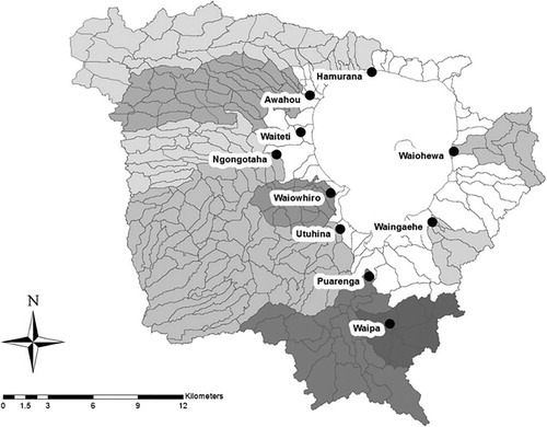
The geology of the Rotorua catchment is complex comprising three separate ignimbrite layers punctured by rhyolite domes, with sedimentary rocks around the lake (White et al. 2007). Aquifers occur in all four formations, and groundwater makes a significant contribution to lake inflow (Pang et al. 1996; Beya et al. 2005; White et al. 2007). White et al. (2014) estimated the area of the surface catchment to be 502 ± 3 km² (mean ± 95% CI) and concluded from the water balance that drainage from outside the surface catchment flowed as groundwater into the Waiteti, Awahou and Hamurana streams (Figure 1). The area of the groundwater catchment was estimated to be 537 ± 26 km² and its outer boundary was mapped with uncertainties of −640 to + 740 m in the Awahou and Waiteti, ± 200 m in the Hamurana and ± 20 m elsewhere (McMillan et al. 2017).

Figure 1. The groundwater catchment of Lake Rotorua as determined by White et al. (2014). Also shown are the 280 sub-catchments used in the ROTAN model. Shading denotes the recharge zones draining to the 10 monitoring sites, indicated by black dots. Unshaded denotes ungauged sub-catchments. Circles denote flow and water quality monitoring sites.

Taylor et al. (1977) showed that springs around Lake Rotorua contained old groundwater. Morgenstern et al. (2004, 2015) found that water ranges in age from 14–170 years in groundwater bores and from 30–145 years in major springs and streams ranges. NO₃–N is readily transported into groundwater and could take years-decades to reach the lake. Williamson et al. (1996) compared stream loads in 1988–1989 (post-KCCS) and 1976–1978 (pre-KCCS) in the Ngongotaha Stream. Ten–twelve years after retirement particulate nitrogen (PN) loads had declined by 20%–30% but NO₃–N loads had increased by 25%. Williamson suggested that NO₃–N was making its way slowly through the groundwater following land use intensification in the 1950–1960s.

Groundwater flow models have been developed in several New Zealand catchments to help manage water resources and contaminants. Particle tracking algorithms in such models help identify recharge zone boundaries, groundwater flow pathways and travel times from land parcels to where groundwater re-emerges (Baalousha 2010; Rutherford 2011). GNS-Science has developed groundwater models for the Rotorua catchment (White et al. 2007; Daughney et al. 2015) and preliminary maps showing particle tracks and travel times have been sighted, but further work is needed to finalise results (Paul White, GNS-Science, pers. comm.).

Attenuation

OVERSEER does not consider the fate of N after it leaves the farm. However, after leaving the root zone, leached N can be transformed, stored, released or lost. These transformations and losses (collectively termed ‘attenuation’) can occur in the vadose zone (through plant and microbial uptake), groundwater (through denitrification, especially where organic carbon is present and oxygen low), wetlands (through plant uptake and denitrification) and streams (through aquatic plant uptake). Alexander et al. (2002) found that the proportion of N losses reaching the catchment outlet (viz., the proportion attenuated) varied from 39%–45% in three Waikato catchments (land area 2833 km²–4614 km² c.f., 424 km² at Rotorua). A mechanistic model of catchment-scale attenuation would require a quantitative understanding of the various pathways that N follows between the root zone and the lake, together with the transformations and losses along each pathway. Currently, there is not enough information available to build such a model.

Available catchment models

OVERSEER estimates the nutrient losses from individual land parcels, but to estimate lake loads it is necessary to route losses to the lake accounting for attenuation and groundwater lags. We reviewed several existing models at the start of this study. Cichota and Snow (2009) examined 17 nutrient models relevant to New Zealand pastoral farms. Eleven operate at the point/paddock or paddock/farm scale, do not route farm losses to the lake, but could have been used in place of OVERSEER had Council wished. Five of the models operate at the scale of farm/catchment or catchment (SPARROW, CLUES, EnSus, AquiferSim and ROTAN). SPARROW (Alexander et al. 2002) estimates nutrient yield coefficients for two farm types (drystock and dairy), together with attenuation coefficients that vary with stream size, to predict annual stream TN and TP loads. Both yields and attenuation coefficients were calibrated by matching stream observations across sampling site networks. CLUES (Woods et al. 2006a) incorporates OVERSEER and SPARROW and predicts steady-state TN and TP loads at the catchment scale. SPARROW and CLUES do not currently account for groundwater lags and are best suited to estimating steady-state loads for constant land use, although groundwater is being added to CLUES (Sandy Elliott, NIWA, pers. comm.). The EnSus framework (Stephens et al. 2003) allows a risk assessment to be made that different land uses pose to soils and water quality but it does not provide a means to accumulate, route and attenuate nutrient losses to the lake. AquiferSim (Bidwell and Good, 2007) operates at a regional scale and calculates N leaching and concentrations in groundwater. Its groundwater algorithms would be suitable as part of a catchment model, but it would need to be modified to incorporate OVERSEER losses, together with quickflow and streamflow delivery pathways. ROTAN is based on HBV-N, a conceptual rainfall-runoff model developed during the 1970s in Scandinavia (Bergström 1995) that has been extended to simulate N (Pettersson et al. 2001). ROTAN is described in more detail below.

Morgenstern et al. (2015) used the exponential piston-flow model (EPM) to estimate groundwater ages (reported as mean residence times, MRT) from atmospheric tracers (notably tritium) measured in springs, streams and bores at Rotorua. Morgenstern and Gordon (2006) then used the EPM model to predict the effects of a step change in farm losses on N loads to Lake Rotorua. However, they only considered groundwater, neglected overlandflow and interflow, assumed land use was spatially homogeneous, and simplified the progressive changes in farm losses to a step increase. ROTAN incorporates the EPM model as described below.

Tuo et al. (2015) compared five catchment-scale models commonly used overseas: SWAT, SWIM, GWLF, AnnAGNPS and HSPF. They found that data availability was a crucial factor in evaluating model results and uncertainty in these process-based models, and that in many situations models were difficult or impossible to implement due to the limited available data. The same argument applies to models like MIKE-SHE and ANSWERS. INCA (Wade et al. 2002) is a process-based model of the N cycle in the plant/soil and stream systems that simulates the N export from different land-use types and predicts stream NO₃–N and ammonium (NH₄–N) concentrations at a daily time-step. It has its own in-built N loss algorithms developed for European farming systems which are untested in New Zealand and cannot easily be replaced by OVERSEER.

Using the selection criteria outlined by Tuo et al. (2015) we concluded that none of the available process-based models was well-suited for application in Rotorua, where there was only limited data. This decision is supported by a recent study using SWAT in the Puarenga catchment (Me et al. 2015). They calibrated SWAT using monthly stream monitoring data from 2004–2008 and validated it using monitoring data from 1994–1997, and high-frequency storm measurements. The model under-estimated storm loads (because baseflows were over-represented in the calibration data) and model parameters varied between baseflow and stormflow conditions, which highlights the difficulty of calibrating a complex model using commonly available data. Significantly, SWAT does not model regional groundwater and so was unable to predict the effects of land use intensification or changes over time in N losses from the land disposal site.

Both N and P influence lake water quality (Hamilton et al. 2012). However, this study focuses on N with the aim of quantifying how groundwater lags and the intensification of farming have affected lake N loads, and to forecast the effectiveness of proposed measures to reduce N losses in the catchment. Phosphorus is transported principally in overlandflow and interflow, groundwater lags are of secondary importance for managing anthropogenic P and models that do not include groundwater (e.g. CLUES and SWAT) are suitable. The main objective of this study is to assess the risk that proposed measures to reduce N losses in the Rotorua catchment will be less (or more) than required to meet the target lake N load.

Methods

ROTAN

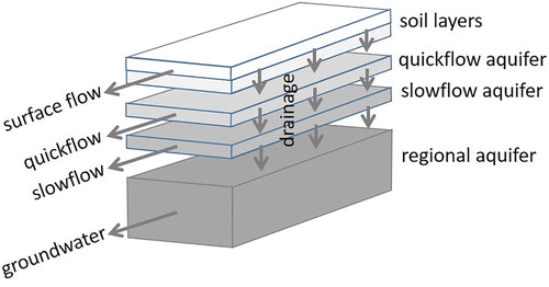
Of the model frameworks reviewed, the most suitable for this study was deemed to be HBV-N for three reasons: it can use OVERSEER loss estimates, it includes groundwater, albeit in a conceptual framework and it runs quickly, making it amenable to calibration and sensitivity analysis. HBV-N simulates groundwater flow using linear reservoirs stacked vertically (Figure 2) that can be linked in series and parallel. We programmed a two-layer version of HBV-N in VBA within EXCEL. An annual time step was considered appropriate because the target lake load is specified as an annual load, the mean residence time of the lake is 450 days (White 1977), OVERSEER calculates long-term average losses, and part of the load to the lake is delivered via groundwater with annual-decadal lag times.

Figure 2. Schematic of the original HBV model.

Hydrology

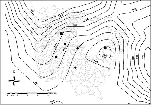
Version 2 of the River Environment Classification (REC) (Snelder and Biggs 2002, www.niwascience.co.nz/ncwr/rec) was used to define 280 sub-catchments containing stream reaches 2nd-order or higher in the groundwater catchment of Lake Rotorua (Figure 1). In each sub-catchment annual runoff was calculated (rainfall minus actual evapotranspiration AET). Annual rainfall has been measured at various locations within the Rotorua catchment since 1900 (http://cliflow.niwa.co.nz). Although no site has operated for the entire period, there were adjacent sites with sufficient overlap to establish correlations and produce a time-series of ‘reference’ rainfall. Rainfall in each sub-catchment was estimated by scaling the reference rainfall using a contour map of 30-year average rainfall (1981–2010) (Figure 3). The scaling factors were the 30-year average rainfall in the sub-catchment divided by the average reference rainfall, assumed constant over time.

Figure 3. Contours of average rainfall 1981–2010. Also shown are the REC2 sub-catchments and the outer boundary of the groundwater catchment. In the north-west streams flow away from the lake but drainage is assumed to reach the lake. Major springs are shown as circles. The reference rainfall gauges are shown as squares. Source: https://www.niwa.co.nz/climate/research-projects/national-and-regional-climate-maps

Annual actual evapotranspiration (AET) was estimated following Zhang et al. (2001).(1) where w is the available water coefficient (dimensionless). Daily potential evapotranspiration (PET) was calculated from meteorological data at Rotorua Airport from 1970–2015 using FAO-Penmann for pasture (Allen et al. 1998), modified Penmann–Monteith for the forest (Whitehead and Kelliher 1991) and Jobson (1975) for open water, and the annual average PET calculated. Prior to 1970, there were no data from which to estimate PET and a synthetic AET time-series was generated by looping the 1970–2015 data.

Nitrogen losses

A companion paper (Palliser et al. in press) describes how historic nitrogen losses from farmland and forest were estimated using OVERSEER v6.2.0 using published agricultural statistics, land cover and land use maps, aided by expert opinion about changes in farm location and practice. Using land use maps for 1900, 1940, 1958, 1974, 1986, 1996, 2003 and 2015, annual average OVERSEER nitrogen yields (kg ha⁻¹ y⁻¹) were estimated for 2000–3000 farm ‘blocks’ (i.e. land areas with the same soils, rainfall, stocking rate, animal breeds, effluent disposal and fertiliser use). Block losses (kg y⁻¹) were calculated, summed within each of the 280 REC sub-catchments and point source loads (from the WWTP, septic tanks, urban areas and geothermal sources) added. In years without land use maps losses were estimated by linear interpolation. Palliser et al. (in press) calculated OVERSEER block losses from(2) with an uncertainty assumed to be randomly, normally distributed with zero mean(3) where is the N yield from block i (kg ha⁻¹ y⁻¹), is the OVERSEER N yield from block i (kg ha⁻¹ y⁻¹), is the scaling factor applied to estimates made for ‘typical’ farms, is the error variance, is the uncertainty in the OVERSEER model, is the variation between farms, and is the uncertainty of the input data to OVERSEER.

Routing and nitrogen attenuation

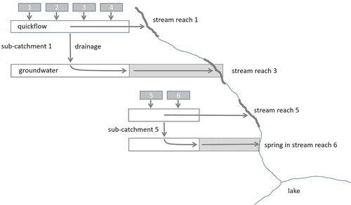
In ROTAN a new conceptual model was added to HBV-N and used to route water and nitrogen from land to the lake along three pathways (quickflow (viz., overlandflow plus interflow), groundwater and streamflow) and to quantify attenuation along each pathway. Appendix A1 gives a summary of the model equations. Total runoff from each land parcel was split into quickflow (in the top layer) and groundwater (in the bottom layer) (Figure 4). For each land parcel and year, the initial N concentration was calculated from N yield (kg ha⁻¹ y⁻¹) divided by runoff (mm y⁻¹) and assumed identical in quickflow and groundwater.

Figure 4. Schematic of the ROTAN model. Each REC sub-catchment contains farm blocks (1, 2, 3, etc.) whose nitrogen loss is estimated using OVERSEER. Nitrogen losses are summed in each sub-catchment and sub-divided into quickflow (which enters the stream reach in the sub-catchment it is generated in the year it is generated), and groundwater (which may enter a different stream reach years-decades after being generated). Quickflow and groundwater eventually reach a stream reach and are accumulated along the stream network.

In the REC there is a stream reach defined for each sub-catchment (Figure 4). Quickflow was assumed to travel to the stream reach in the sub-catchment where it was generated, in the year it was generated (viz., no time lag) and attenuation was assumed to be first-order in distance (Appendix A1, Equation A10). Groundwater was assumed to travel via a streamtube to a spring, stream reach or the lake (Figure 4) and attenuation was assumed to be first-order in travel time (Appendix A1, Equations A3–A5).

Recharge zones were estimated for each of the 10 flow recorders using water balances (Figure 1), following White et al. (2007) but using slightly different rainfall and streamflow data. Groundwater from all REC sub-catchments within a recharge zone were assumed to re-emerge at the flow recorder, with only quickflow contributing to streamflow above the recorder. In ungauged catchments, groundwater was assumed to re-emerge in the stream reach immediately downstream. Following White et al. (2007), each recharge zone was assumed to comprise land upslope from, and contiguous with, the flow recorder (i.e. aquifers were assumed to be unconfined with homogeneous geology). The ‘drainage fraction’ (viz., the proportion of runoff draining to groundwater) was assumed identical for all land parcels in a recharge zone and constant over time, but could vary between recorders. The drainage factors were calculated as the ratio of baseflow to total flow at each of the flow recorders, where baseflow was calculated as the average of the minimum streamflow in each three-month period. Ungauged sub-catchments were assigned the average drainage factor for the 10 recharge zones.

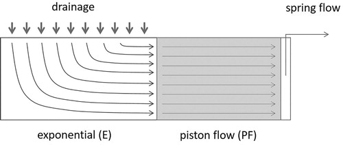
The EPM assumes complete mixing of recharge in the unconfined aquifer (the exponential E component) followed by piston flow in the confined aquifer (the PF component) (Figure 5). The E component of the model contains the coefficient which smooths out the effects of year-to-year variations of drainage on streamflow (Appendix A1, Equations A1–A2). For water, inflow equalled outflow for the piston flow (PF) component of the model (viz., no time delay) but for nitrogen, the EPM introduces a time lag. The time lag (MRT) for each streamtube was assumed to vary linearly with the distance between the sub-catchment and the spring.

Figure 5. Schematic of the EPM model used to estimate groundwater age (Morgenstern et al. 2015) and to route water and nitrogen from each sub-catchment to the stream network or lake in ROTAN.

For each year of the simulations, annual quickflow and any re-emerging groundwater were accumulated along the stream network. The lake was included which enabled measured lake outflows to be used to calibrate w in the Zhang model (Equation 1). Because travel times in the stream network were orders of magnitude less than the model time step, nitrogen mass inflows (from quickflow and upwelling groundwater) were also accumulated along the stream network. Streamflow attenuation was assumed first-order in distance, and to vary inversely with the flow (following Viner 1987) (Appendix A1, Equations A11–A12).

Stream and groundwater nitrogen concentrationsfish

Nitrogen concentrations in 10 major and 8 minor streams have been measured intermittently since the late 1960s (Fish 1975; Hoare 1980; Williamson et al. 1996) typically at monthly intervals with several large gaps (see Appendix A3 for a summary of available monitoring data). Streamflows have been measured continuously at some of the sampling sites, and gauged at the time of sampling at others, again with several gaps. Prior to 1990 studies report NO₃–N, NH₄–N, nitrite (NO₂–N) and dissolved inorganic nitrogen (DIN = NO₃–N + NO₂–N + NH₄–N) but few particulate (PN), dissolved organic (DON) or total nitrogen (TN) concentrations. NH₄–N and NO₂–N concentrations were found to be consistently low in spring and stream water meaning that NO₃–N gives a good indication of DIN. There is limited temporal coverage in the available groundwater chemistry data. GNS-Science sampled 12 bores in July 2003 as part of a water age study (Morgenstern et al. 2004). White et al. (2007) list 169 bores or springs, but most were sampled only once between 2003 and 2006 and routine monitoring has only occurred at two sites.

Calibration

ROTAN was calibrated to measured stream TN concentrations (NO₃–N + NO₂–N + NH₄–N + DON + PN). Concentrations used in calibration were flow-weighted averages of TN from routine sampling in which baseflows are over-represented, although there are occasional high flow measurements. In each calibration run, attenuation coefficients were sought to minimise the root mean square (RMS) percentage error at the 10 stream monitoring sites.(4) where prd is the predicted TN concentration (g m⁻³) and obs is the flow-weighted average stream TN concentration (g m⁻³). The summation was over 3–4 years in each of eight sampling periods from 1975–2015. A grid search was used, with constraints on attenuation coefficients imposed based on published stream and groundwater attenuation.

The available water coefficient w in Equation 1 was calibrated to match predicted and observed flows at the lake outlet, with the difference between forest and pasture w values fixed at 0.1 to ensure that AET was greater for forest than pasture (Whitehead & Kelliher 1991). The boundaries of the recharge zones were estimated to achieve a water balance at each flow recorder. The external groundwater boundary defined the northern and western boundary of the Hamurana recharge zone (Figure 1). REC sub-catchments were added or removed (by trial and error) along the southern boundary of the Hamurana recharge zone until observed and predicted flows matched at the Hamurana recorder. The same process was followed in adjacent catchments moving counter-clockwise around the lake. The values of which smooth out the effects of year-to-year variations of drainage on streamflow (Appendix A1, Equations A1–A2) were assumed spatially homogeneous in each recharge zone, and calibrated to match measured year-to-year variations in streamflow. For each of the streamtubes draining to a site where water age had been measured, the parameters of the EPM models (Appendix A1, Equations A6–A9) were calibrated so that the flow-weighted average of the streamtube MRTs matched the published MRT for the site (Table 1). Ungauged sub-catchments were assigned a default MRT of 5 years.

Table 1. Mean residence times (MRT) from Morgenstern et al. (2015) estimated by fitting binary exponential (E) piston flow (PF) models (EPM) to tritium measurements in the major stream inflows to Lake Rotorua.

Stream	MRT year	%
Hamurana (HAM)	125	82, 77 (80)
Awahou (AWA)	75	100, 91 (99)
Waiteti (WTT)	45	100, 90 (98)
Ngongotaha (NGO)	30	100, 91 (98)
Waiowhiro (WWH)	40	63 (63)
Utuhina (UTU)	60	60, 100 (79)
Puarenga (PUA)	40	100, 100 (100)
Waingaehe (WNG)	145	94, 100 (95)
Waiohewa (WHE)	40	100, 100 (100)

Note: ϵ is the proportion of exponential flow. Column 3 contains ϵ values for the two EPM models fitted by Morgenstern and the weighted average (brackets) used in ROTAN.

Two assumptions were made concerning attenuation coefficients.

Spatially-homogenous attenuation (SHA)

Attenuation was assumed to be spatially homogeneous across the entire watershed. The model was calibrated to minimise the flow-weighted value of across the 10 monitoring sites. Calibrations were retained where  ≤ 10%.

Spatially-variable attenuation (SVA)

Attenuation was assumed to be spatially homogeneous within each sub-catchment draining to a stream monitoring site, but to vary between monitoring sites. The model was calibrated to minimise at each of the 10 monitoring sites. Calibrations were retained where  ≤ 15% which approximates the uncertainty in annual average flow-weighted stream TN concentration.

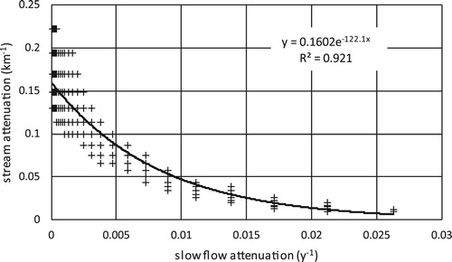
During calibration, constraints were imposed on the feasible range of attenuation coefficients using published information (Table 2). Viner (1987) summarised stream attenuation coefficients measured in New Zealand streams (Figure 6) which indicate likely bounds of 0.01 <  < 0.45 km⁻¹ and justify fixing  = −0.7 (Appendix A1, Equations A11–A12). Morgenstern et al. (2004) report DIN concentrations and water age (MRT) for bores and springs studied in 2003 (Table 3). These data were used, together with estimates of drainage (50% of catchment rainfall) and nitrogen loss (from OVERSEER using historic land use data), to make a priori estimates of the groundwater attenuation coefficient (see Appendix A1, Equations A13–A14). It was not possible to make a priori estimates of the quickflow attenuation coefficient and so a wide range was assumed.

Figure 6. Reported stream attenuation coefficients from Viner (1987). This study re-examined the data in Viner (1987). The solid line refers to Equation A12 and was fitted by log-log regression. The dashed lines enclose 95% of observations. Upper dashed α = 0.45, middle solid  = 0.095 and lower dashed  = 0.01. Slope  = −0.705 for all lines.

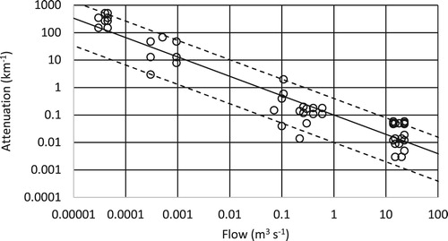
Table 2. A priori upper and lower bounds on model attenuation coefficients based on published values.

Coefficient	Symbol	Units	Max	Min	Equation
Slow flow		y^−1	1.0E−02	1.0E−04	A3, A5
Quick flow		km^−1	10	0.01	A10
Stream		km^−1	0.45	0.01	A11–A12

Table 3. Groundwater and spring data used to make a priori estimates of the slow flow attenuation coefficient σ (Appendix A1 Equations A13 and A14). No and MRT are from Morgenstern et al. (2004). D and N_d are from this study. L is the estimated loss MRT years prior to 2003 from this study. Where Equation A14 gave a negative value it was assumed that  = 1.0E−04.

Site	No	L	MRT	D	Nd	σ
	mg m^−3	kg ha^−1 y^−1	y	mm y^−1	mg m^−3	y^−1
Hamurana spring	735	8	150	1100	727	0.0001
	735	9	150	1100	818	0.0007
	735	10	150	1100	909	0.0014
Awahou spring	1410	10	64	1100	909	0.0001
	1410	15	64	1100	1364	0.0001
	1410	20	64	1100	1818	0.0040
Hatchery spring	945	5	54	1100	455	0.0001
	945	10	54	1100	909	0.0001
	945	15	54	1100	1364	0.0068
Barlows spring	567	5	73	1100	455	0.0001
	567	10	73	1100	909	0.0065
	567	15	73	1100	1364	0.0120
Bore 2116	223	3	135	1050	286	0.0018
	223	5	135	1050	476	0.0056
	223	10	135	1050	952	0.0108
Bore 1561	606	3	112	950	316	0.0001
	606	5	112	950	526	0.0001
	606	10	112	950	1053	0.0049
Bore 3691	847	3	94	1100	273	0.0001
	847	5	94	1100	455	0.0001
	847	10	94	1100	909	0.0007
					Median	0.0007
					25% quartile	0.0001
					75% quartile	0.0050

Results

Flow

Coefficients w = 1 (pasture) and w = 1.1 (forest) in Equation 1 gave an RMS error for the lake outlet of 8% (Table 4) which is within the accuracy of measured flows. The recharge zone boundaries of the flow sites were adjusted until the median RMS error was 10% (Table 4). Predicted drainage averaged 50% of rainfall (range 41%–59% between wet and dry years) which matched the average value of 51% measured using lysimeters in the northern part of the catchment (White et al. 2007; Freeman 2010). Annual runoff averaged 996 ± 38 mm y⁻¹ (mean ± 95%CI) which fell within the band 800 mm y⁻¹–1000 mm y⁻¹ mapped by Woods et al. (2006b) and was comparable with the average of 927 ± 40 mm y⁻¹ calculated using their alternative form of the Zhang equation. After calibrating the coefficient in the exponential component of the EPM model (Appendix A1, Equations A1–A2) ROTAN matched the observed year-to-year variations in flow at the 10 flow sites (Figure 7).

Figure 7. Observed (obs) and predicted (prd) annual average flow in five of the major inflows and the lake outlet. Figure 1 shows site locations and name codes.

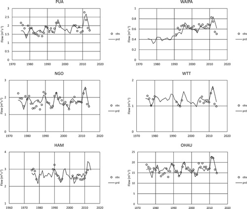
Table 4. Average observed flow and RMS difference between observed and predicted annual flow, after calibration.

Site	Code	Observed mean flow m^3 s^−1	RMS error m^3 s^−1	RMS error %	Number of years
Lake outlet	OHAU	16.79	1.39	8%	40
Hamurana	HAM	2.65	0.21	8%	22
Awahou	AWA	1.62	0.12	7%	21
Ngongotaha	NGO	1.79	0.20	11%	40
Puarenga	PUA	1.83	0.21	12%	33
Utuhina	UTU	1.84	0.23	12%	32
Waingaehe	WNG	0.25	0.02	9%	20
Waiowhiro	WWH	0.32	0.05	16%	15
Waiohewa	WHE	0.36	0.03	9%	18
Waiteti	WTT	1.22	0.13	11%	19
Waipa	WAIPA	0.64	0.08	12%	24

Farm losses

When farms were modelled in OVERSEER using both detailed ‘benchmarking’ and ‘generic’ data for 2003, the former gave higher nitrogen losses. Consequently, all pre-2003 losses calculated using ‘generic’ farm data were scaled by  = 128% (dairy), 139% (dry stock) and 133% (mixed) (Equation 2). The differences between ‘benchmarking’ and ‘generic’ estimates of farm losses in 2003 may reflect recent farming practices, and had the differences been lower from 1900 to 1995, ROTAN would overestimate historic farm losses. Analysis of variance of the 2003 ‘benchmarking’ losses quantified the variation between similar farms to be = 25% (dairy) and = 30% (dry stock) and these values were used for pre-2003 farms. At test sites where nitrogen losses have been measured, the reported uncertainty in OVERSEER averages = 30% (Selbie et al. 2003) which was assumed for all farms (see Equation 3). In 2003 and 2015,  = 1 and  = 0, and although  = 0, variations between farms were captured in the ‘benchmarking’ data of .

Spatially homogeneous attenuation (SHA)

Table 5 shows the RMS error (viz., goodness-of-fit) at the 10 monitoring sites, and the flow-weighted average for the SHA calibration. The flow-weighted median RMS error across all 10 sites was only 1% but the model significantly over-estimated TN concentrations (RMS > 15%) at two sites (AWA and NGO) and under-estimated them at five sites (PUA, UTU, WHE, WNG and WWH). To illustrate key features of the SHA calibration, Figure 8 shows observed and predicted annual average TN concentrations at a selection of stream monitoring sites for one combination of calibrated attenuation coefficients. In 1991 land treatment of wastewater commenced in the WPA and the model successfully predicted the significant increases in TN concentration. Predictions under-estimated observations in the PUA and did not capture the apparent decrease in observed concentrations from 2000 to 2012. The reasons for this mismatch are unclear. There are several springs in the NGO and WTT catchments where water has been aged at 30–45 years. Land use intensification occurred in both catchments in the late 1940s, has continued in the WTT but has decreased in the NGO with the spread of peri-urban lifestyle blocks. The model captured the trend and magnitude of changing TN concentrations. The AWA and HAM catchments both contain large springs with old groundwater (75–125 years). There has been a significant expansion of dairy farming in the AWA in the last 30 years but the model significantly over-estimated TN concentrations. There may be errors in the boundaries of the AWA recharge zone but there is not enough information about the hydrogeology of the catchment to guide making changes. It is possible that farm losses have not yet reached the steady-state OVERSEER values in the AWA recharge zone, although the intensification started in the 1980s. Flow in the HAM is predominantly groundwater from an aquifer northwest of the lake. The headwaters are indigenous forest but there is farmland in the middle and lower parts of the catchment. Despite significant groundwater lags, there is an increasing trend in both observed and predicted concentrations. For other combinations of calibrated attenuation coefficients, the match between observed and predicted concentrations differed in detail from those shown in Figure 8, but the general patterns remained unchanged.

Figure 8. Observed annual flow-weighted mean TN (obs) and predicted (prd) concentrations in six of the major stream inflows. Attenuation coefficients were spatially homogeneous (SHA calibration) with σ = 5.0E−03 y⁻¹, κ = 0.05 km⁻¹ and α = 0.1 km⁻¹. Goodness-of-fit is summarised in Table 5. Figure 1 shows site locations and name codes.

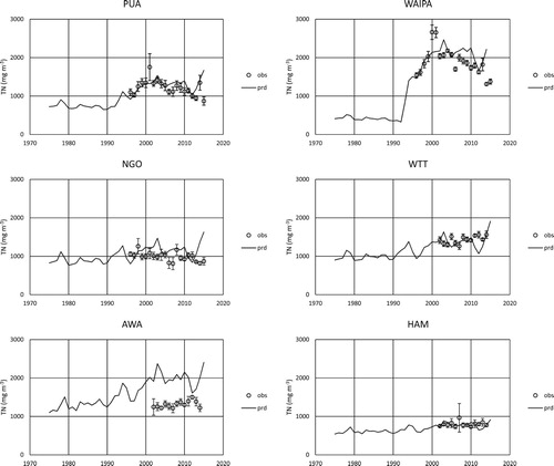
Table 5. Spatially homogenous attenuation (SHA): Summary of goodness of fit after calibration assuming homogeneous attenuation coefficients. The goodness of fit parameter is defined in Equation (4). The calibrated attenuation coefficients (median (interquartile range)) were: groundwater σ = 0.0016 (0.0004–0.0073) y⁻¹, streamflow α = 0.130 (0.066–0.170) km⁻¹ and quickflow κ = 0.1 km⁻¹. Note that σ and α were inversely correlated.

	AWA	HAM	NGO	PUA	UTU	WHE	WNG	WTT	WWH	WAIPA	Flow weighted
Flow m^3 s^−1	1.63	2.65	1.79	1.83	1.84	0.36	0.25	1.22	0.33	0.64
	RMSE
Min	24%	−27%	−15%	−45%	−35%	−65%	−58%	−20%	−36%	−39%	−10%
25%ile	49%	−6%	14%	−33%	−28%	−48%	−46%	−15%	−27%	−20%	−5%
Median	56%	7%	16%	−24%	−25%	−39%	−39%	−12%	−22%	−13%	−1%
75%ile	63%	12%	18%	−14%	−23%	−30%	−32%	−8%	−17%	11%	4%
Max	80%	26%	38%	40%	−18%	−13%	−15%	10%	−8%	30%	10%
Count	923	923	923	923	923	923	923	923	923	923	923

Predicted concentrations were insensitive to quickflow attenuation because drainage factors were high in most sub-catchments and quickflow was only a small proportion of total runoff. The groundwater and stream attenuation coefficients were strongly, inversely correlated (Figure 9). For example, equally good fits were obtained with upper bound groundwater and lower bound stream attenuation, lower bound groundwater and mid-range stream attenuation, and several intermediate combinations.

Figure 9. Calibrated slow flow and stream attenuation coefficients assuming spatial homogeneity across the catchment.

Spatially variable attenuation (SVA)

The model was also calibrated assuming that attenuation varied between monitoring sites but was spatially homogeneous across land parcels draining to the same monitoring site. Given the a priori constraints on attenuation, it was possible to calibrate the model to  ≤ 10% at 5 monitoring sites (AWA, HAM, WHE, WTT and WWH) and to  ≤ 15% at the other 5 sites (Table 6). In the HAM and WWH, springs emerge close to the lake shore and the stream is not long enough for significant stream attenuation. In most sub-catchments observed and predicted concentrations matched more closely than in Figure 8 although in several sub-catchments significant discrepancies remained.

Table 6. Spatially-variable attenuation (SVA): Calibrated attenuation coefficients and goodness of fit after calibration assuming variable attenuation coefficients. Summary statistics are given for the groundwater and streamflow attenuation coefficients but the quickflow attenuation coefficient does not affect predicted stream TN concentrations and is omitted. The goodness of fit parameter is defined in Eq. 3. Note that and are inversely correlated. The flow-weighted RMSE across all 10 sites averaged  = −4% (inter quartile range −10% to 10%).

	Slow	Stream	RMSE	Slow	Stream	RMSE	Slow	Stream	RMSE	Slow	Stream	RMSE	Slow	Stream	RMSE
	AWA			HAM			NGO			PUA			UTU
min	0.011	0.010	−10%	0.0001	0.010	−10%	0.0001	0.020	−15%	0.0001	0.013	−15%	0.0001	0.010	−15%
25%ile	0.021	0.026	−7%	0.0006	0.044	−6%	0.0006	0.099	−14%	0.0005	0.044	−13%	0.0003	0.017	−14%
median	0.026	0.099	5%	0.0025	0.148	5%	0.0025	0.170	−13%	0.0028	0.058	−10%	0.0009	0.022	−13%
75%ile	0.032	0.255	7%	0.0038	0.255	7%	0.0112	0.255	14%	0.0138	0.076	12%	0.0025	0.029	14%
max	0.040	0.5	10%	0.0073	0.437	10%	0.0500	0.334	15%	0.0500	0.099	15%	0.0112	0.044	15%
count	59	59	59	232	232	232	199	199	199	146	146	146	168	168	168
	WHE			WNG			WTT			WWH			WPA
min	0.0001	0.010	−10%	0.0001	0.010	−15%	0.0001	0.010	−10%	0.0001	0.010	−10%	0.0001	0.010	−15%
25%ile	0.0003	0.015	−9%	0.0002	0.022	−13%	0.0004	0.044	−6%	0.0003	0.026	−7%	0.0006	0.058	−13%
median	0.0007	0.017	−9%	0.0006	0.034	−12%	0.0013	0.066	−4%	0.0010	0.039	−6%	0.0047	0.076	11%
75%ile	0.0020	0.022	9%	0.0015	0.044	13%	0.0047	0.099	6%	0.0031	0.058	7%	0.0212	0.099	13%
max	0.0059	0.029	10%	0.0038	0.066	15%	0.0404	0.170	10%	0.0112	0.087	10%	0.0500	0.130	15%
count	119	119	119	127	127	127	252	252	252	187	187	187	211	211	211

The calibrated attenuation coefficients varied by 2 orders of magnitude (Table 6) and yet TN concentrations were predicted to within 10% or 15%. The reason is that groundwater and streamflow attenuation coefficients were negatively correlated. As a result, an equally good fit between observed and predicted stream TN concentrations was achieved with low groundwater and high streamflow attenuation, or high groundwater and low streamflow attenuation.

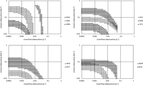
There were significant differences in calibrated attenuation between sub-catchments (Figure 10). For example, in the PUA, NGO and UTU, for median groundwater attenuation (σ < 0.001 y⁻¹) stream attenuation varied significantly (0.017 < α < 0.29 km⁻¹). In the UTU and WHE calibrated stream attenuation coefficients were near the lower limit of published values (Table 2) and lower than in other streams (Figure 10). In the AWA calibrated attenuation coefficients were near the a priori upper bound and yet TN concentrations were over-estimated.

Figure 10. Spatially variable attenuation (SVA). The correlation between calibrated groundwater and streamflow attenuation coefficients. Attenuation coefficients were calibrated separately in each of the 10 major sub-catchments: Awahou (AWA), Hamurana (HAM), Waingaehe (WNG), Puarenga (PUA), Ngongotaha (NGO), Utuhina (UTU), Waiohewa (WHE), Waiteti (WTT), Waiowhiro (WWH) and Waipa (WPA). Goodness of fit is summarised in Table 6.

Catchment-scale attenuation (i.e. the difference between total N losses and total lake inflow) was calculated for all combinations of coefficients. Attenuation averaged 42% (range 23%–50%) which compares favourably with published values (Alexander et al. 2002).

Calculations of lake nitrogen loadings

Council has consulted with stakeholders and proposes to reduce N lake loads by reducing N losses in the catchment in three phases (with reduction targets for the years 2020, 2027 and 2033) giving a total reduction in losses of 531 t y⁻¹ (BoPRC 2017). Proposed reductions from farmland are 188 t y⁻¹ through incentives and 263 t y⁻¹ through new rules, with an additional 100 t y⁻¹ reduction from point sources plus gorse control. ROTAN was used to investigate whether these reductions are likely to meet the target lake N load.

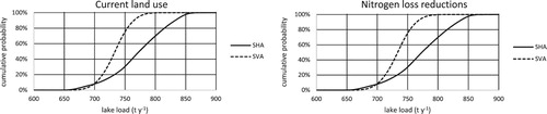
Firstly, steady-state lake loads were calculated assuming current losses by running the model with numerous combinations of calibrated attenuation coefficients. Figure 11 (left) shows the frequency distribution of the predicted steady-state load for current land use. The 50%ile load lies in the range 754 ± 39 t y⁻¹ (mean ± 95% confidence interval) meaning that significant reductions will be needed to achieve the target lake N load (405 t y⁻¹). Second, the proposed scenario of nitrogen loss reductions was modelled (Figure 11, right). The 50%ile load lies in the range 431 ± 26 t y⁻¹. There is a 12%–18% probability that the load will be less than the target (viz., loss reductions are more than required). On the other hand, there is an 82%–88% probability that the lake load will exceed the target (viz., loss reductions are less than required). It was beyond the scope of this study to examine the implications for lake water quality of not reaching the target lake N load. However, it might be reasonable to assume that lake water quality will be significantly improved provided the lake load is within 5% of the target (viz., within the range 385 t y⁻¹–425 t y⁻¹). For the SHA and SVA calibrations the probabilities that lake load will be < 425 t y⁻¹ are 27% and 76%, respectively.

Figure 11. Frequency distribution of calculated steady-state lake load (SHA and SVA calibrations) assuming current land use (left) and the nitrogen loss reductions proposed by Council (right).

ROTAN was used to predict the trajectory of lake load assuming current land use and the proposed scenario of nitrogen loss reductions. Figure 12 compares predicted lake loads from 1900–2015 with published load estimates. The 1900 estimates of 90 t y⁻¹ (Morgenstern and Gordon 2006) and 206 t y⁻¹ (McIntosh in BoPRC 2009) differ significantly (Table 7). The former is based on measured N concentrations in very old groundwater, while the latter is based on modern day N yields from undeveloped land. The 1970 estimate of 232 t y⁻¹ (Fish 1975) is for DIN whereas other loads are for TN and is omitted from Figure 12. Abell et al. (2015) estimated annual TN loads from 2007–2014 and we estimated the year-to-year variation in their loads to average 15%–the uncertainty shown in Figure 12. Since 1900 there have been irregular changes in the areas of pasture and forestry, animal type and breed, stocking rate, fertiliser use, effluent disposal etc, with an underlying increasing trend of land use intensification. Population and N loads from domestic wastewater and urban runoff have also increased, with irregular changes in the type and effectiveness of sewage treatment. The effects of these irregular changes on lake nitrogen loads have been delayed and smoothed out where nitrogen losses have entered groundwater. Observed and predicted lake loads match closely (Figure 12, left). Observed and predicted loads were both low from 1995–2000 when land disposal of WWTP effluent commenced which reduced N concentrations in the Puarenga Stream. However, N concentrations in streams not affected by land disposal continued to increase and the benefits of land disposal in terms of reduced lake N loads were short lived. Groundwater lags are such that, were losses to remain unchanged at current levels, lake loads are predicted to increase gradually over several decades before reaching steady state. Our estimates of steady-state load (2100) are comparable with those of Morgenstern and Gordon (2006).

Figure 12. Predicted annual median lake loads from the Rotorua groundwater catchment assuming current land use and the nitrogen loss reductions proposed by Council with upper and lower 95% confidence limits. Also shown is the target load of 405 t y⁻¹ and published estimates of historic loads.

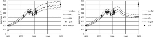
Table 7. Summary of published estimates of phosphorus and nitrogen loads on Lake Rotorua in streams.

	Period	Method	Inflow m^3 s^−1	DRP t y^−1	TP t y^−1	TP t y^−1	TP t y^−1	DIN t y^−1	TN t y^−1	TN t y^−1	TN t y^−1
				streams		WWTP	rain	streams		WWTP	rain
Morgenstern and Gordon (2006)	1900	Model		31	38				90
McIntosh in BoPRC (2009)	1900	Yields			21				206
Rutherford et al. (1989)	1965	Review			34	3			405	30
Fish (1975)	1968–70	1 B	13.5^a	28.1^a		4.4	2.4	232^a,b		27	37
Hoare (1980)	1976	2 A	15.8	24.7	33.7^c	7.5	1.2	376	466^c	68	31
Hoare (1980)	1977	2 A	ND	23.8	32.6^c	8.0	1.0	354	444^c	64	28
Rutherford et al. (1989)	1981–1982				33	21	1		390	134	30
	1984–1985				33	34	1		385	150	30
Beya et al. (2005)	1991–2002	1 A	12–17		35	C	1.3		443	C	29.2
Burger and Hamilton (2005)	2003–2004	1 A	14.2	26.0	33.2	C		442	503	C
McIntosh in BoPRC (2009)	2005	Yields			39.7	C			763	C
Morgenstern and Gordon (2006)	2005	3 A			37.9	C			518	C
	steady state	Model			37.9	C			717^d	C
BoPRC (2009)	2008	Review			37.9	C			526	C
Abell et al. (2015)	2007–2014	2			44.1	C	1.4		595	C	30

Methods: Model = EPM model, Yields = published yield coefficients, Review = expert opinion. 1 = mean concentration x mean flow, 2 = rating curve, 3 = flow-weighted mean concentration x mean flow

A = includes minor streams & ungauged flows, B = excludes minor streams & ungauged flows. C = loss from the RLTS is included in the measured Puarenga Stream loads.

^aminor and ungauged streams excluded.^b1968 nitrate excluded being 50% lower than 1969–1970 values.^cexcludes floodflow particulate loads.^dcurrent land use.

Hoare (1980) includes floods but excludes floodflow particulate loads. Method 1 underestimates the contribution from floods. Method 3 includes any floods sampled. Methods 2 and 4 include floods.

The uncertainty in published loads for the same decade averages ± 15%

The proposed reductions in N losses within the catchment are predicted to significantly reduce lake loads. Predicted 2100 loads are close to, but slightly higher than, the target–as discussed above. Because of groundwater lags, lake loads are predicted to decrease to within 25% of the target 25–30 years after loss reductions, but would not reach steady-state for several decades.

Discussion

Determining the reduction of nutrient losses from diffuse sources to meet water quality targets in catchments with significant groundwater lags poses technical problems because of difficulties estimating historic losses to groundwater, delivery pathways and travel times between individual land parcels and monitoring sites and the lake, and attenuation rates along each pathway. Catchment models need to support decision making but often there is only limited available information to develop and test them, which has two implications. Firstly, the available data may be insufficient to set up, calibrate and test complex physically-based catchment models. Secondly, although simplified models may be more appropriate, their calibration using limited data may result in predictions having large uncertainty. Uncertainty need not be a fatal flaw to decision making, provided it is quantified to the extent that is possible. In this study, we used a simplified catchment model ROTAN running with an annual timestep because the available data was sparse with high uncertainty but the model runs quickly which facilitated sensitivity/uncertainty analysis. Its annual time step is consistent with the target lake load, the time scale of OVERSEER, the residence time of the lake and groundwater lags times. However, when modelling eutrophication in streams where periodic high flows scour aquatic plants, a daily-weekly timestep would be required (Rutherford 2011).

The uncertainty of OVERSEER estimates of N loss from farmland is reported to be ± 30% where input data are known accurately. Palliser et al. (in press) detail historical N losses estimated for this study using agricultural statistics and the limited available information about spatial and temporal changes in farming practice. They estimated the uncertainty in farm losses to average ± 50% which was carried through into ROTAN calibration. The difference (average 88%) in farm losses estimated using OVERSEER v5 and v6 does not affect our findings because OVERSEER v6.2.0 was used throughout the ROTAN modelling reported here.

OVERSEER may not accurately quantify all forms of N leached (notably DON) and it may underestimate N losses during storm events because it does not include streambank or hillslope erosion and appears not to have been calibrated or tested to include storm conditions. Consequently, OVERSEER may underestimate TN losses. Nevertheless, OVERSEER provides a quantitative index of the effects of land use. Shepherd et al. (2009) emphasise its strength in quantifying the effects of changes in farm practice. We take this to mean that OVERSEER estimates of the change in nitrogen losses with a change in land use are more accurate (including being unbiased) than estimates of actual nitrogen losses. This being so, if OVERSEER underestimates N losses, when ROTAN is calibrated against the observed stream and groundwater concentrations, the resulting attenuation coefficients will be underestimates. However, when the model is used to make predictions following land use change using the calibrated attenuation coefficients, there is a reasonable expectation that predictions will be unbiased. Appendix A4 illustrates this argument. Alternative estimates of farm losses could be input into ROTAN (e.g. from ‘lookup tables’ or models such as APSIM (Keating et al. 2003, Lilburne et al. 2010)). If such alternative losses differed from OVERSEER estimates, ROTAN re-calibration would result in changes to its attenuation coefficients. However, because ROTAN is calibrated to measured stream concentrations, we would not expect predicted lake loads to alter significantly.

The target lake N load (405 t y⁻¹) needs to consistent with the stream TN measurements used to calibrate ROTAN. Baseflow conditions are over-represented in the routine stream monitoring used to calibrate ROTAN, although some high flows were sampled. Abell et al. (2012) conducted high-frequency sampling during 17 floods in the Puarenga and Ngongotaha Streams in 2012–2014, and found that omitting the two largest floods only reduced annual TN yields by 6%–7%. Thus, not sampling floods are likely to underestimate the annual load but, based on Abell’s results, the bias is unlikely to exceed 10%. Rutherford et al. (1989) estimated lake load in the 1960s (now the target lake N load) to be the stream load of 455 t y⁻¹ (DIN + DON + baseflow PN) measured in 1976–1977 (Hoare 1980) −50 t y⁻¹ from domestic sewage. Thus, Hoare’s stream load omits flood flow particulates (50 t y⁻¹) which represents 10% of the total load. We conclude that the target lake N load is consistent with the TN loads used to calibrate ROTAN.

If OVERSEER accurately quantifies high farm TN losses during floods, but stream monitoring underestimates stream TN loads, ROTAN calibration will overestimate attenuation. Even if this is the case, we argue that predicted lake loads will be unbiased provided farm losses after mitigation are predicted using OVERSEER together with the calibrated (possibly biased) attenuation coefficients.

The groundwater model in ROTAN is the conceptual EPM model used to analyse rainfall tritium (Morgenstern et al. 2015). Tritium concentrations in rainfall are spatially homogeneous but nitrogen concentrations in drainage vary spatially. Unless the underlying aquifer is well mixed, it is necessary to connect each land parcel to where its drainage re-emerges. In ROTAN a separate streamtube was assumed for each of the 280 REC sub-catchments. The travel time along each streamtube was assumed to vary with distance from the spring, which mimics flow pathways predicted by groundwater modelling and travel time contours estimated from atmospheric tracers. In this study 11 groups of streamtubes (10 for recharge zones draining to a monitoring site, plus 1 for all ungauged sub-catchments) were assigned the same parameters and calibrated to observed flow variability and published MRTs. REC sub-catchments could be aggregated, which would reduce the number of streamtubes and increase the mixing of drainage from different land parcels although this would reduce the range of groundwater travel times.

Although White et al. (2014) define the outer boundaries of the surface and groundwater catchments, there is uncertainty about the location of recharge zones of the aquifers that drain to each of the 10 monitoring sites. This affects our ability to calibrate the nitrogen attenuation coefficients in ROTAN (notably for groundwater). While the area of a recharge zone can be estimated with some confidence (knowing rainfall and spring flow, and assuming recharge is 50% of rainfall as in White et al. 2007), locating its boundary poses challenges. The geology at Rotorua is complex, especially in the north-west of the catchment. For example, the Hamurana Springs lie in a very small surface catchment and upslope from the springs, on the Mamaku Plateau, there are sink holes suggesting preferred flow pathways. Thus, the recharge zone may not be adjacent to, or contiguous with, the recorder as assumed by White et al. (2007) and our water balance calculations. We used slightly different rainfall and stream flow data from White et al. (2007) and consequently derived similar, but not identical, recharge zone boundaries (Rutherford et al. 2011). Spatial variations in rainfall, which are large on the Mamaku Plateau to the northwest of the lake, also mean that several possible recharge zones may match the observed flow. This study was unable to address such complexities. As a result, some land parcels may be ‘connected’ to the wrong monitoring site in ROTAN, which may explain the difficulties encountered calibrating the model in the Awahou catchment. Although groundwater models of the Rotorua catchment exist, further work would be required before they could help refine our estimates of recharge zones (Paul White, GNS-Science, pers. comm.). It may be possible to use geochemical tracers (e.g. stable isotopes) and mixing models to identify water and nutrient sources (Xue et al. 2009) although spatial and temporal variability of farming practice may make it difficult to define unique source signatures, and obtain unique solutions to the mixing equations.

Although ROTAN did not match closely observed stream concentrations in several catchments, the flow-weighted RMSE across all 10 monitoring sites averaged 1%–4% which is within the likely uncertainty of observed stream loads. We argue, therefore, that even if in ROTAN some land parcels drain to the wrong monitoring site, this does not affect the total lake load. Our argument is predicated on attenuation and yields from unmonitored land being similar throughout the Rotorua catchment.

The spatially homogeneous attenuation calibration (SHA) achieved a flow-weighted RMS error of  ≤ 5% although predictions significantly over-estimated observations in some sub-catchments and under-estimated them in others. The variable attenuation calibration (SVA) did not calibrate to within  ≤ 5% at any site, although calibration within  ≤ 10% was achieved at 5 sites and within  ≤ 15% at the remaining 5 sites. In SVA, attenuation coefficients differed significantly between catchments. One might expect differences in groundwater attenuation if the redox chemistry of groundwater varied between aquifers but groundwater data indicates that groundwaters are uniformly well oxygenated (White et al. 2007). Many of the Rotorua streams are similar with incised channels, mobile beds and few aquatic plants. There are no obvious reasons why stream attenuation should vary significantly between streams. It would be unwise, therefore, to rely on the differences in attenuation between sub-catchments identified by SVA (e.g. to seek economically optimal loss reductions) because the differences may be artefacts of inaccurate input data.

When used in Rotorua, the ROTAN model was over-parameterised because there was rather sparse groundwater monitoring data, and calibration of its three attenuation coefficients was based on matching observed stream concentrations, albeit at 10 monitoring sites in different catchments. Predictions were insensitive to quickflow attenuation. Several combinations of groundwater and stream attenuation coefficients gave a similar fit to observed stream concentrations, with calibrated coefficients strongly negatively correlated. Non-uniqueness of calibrated attenuation coefficients cannot be resolved with the available information. Calibrated groundwater attenuation coefficients extended across the full range of the a priori estimates and could not be constrained further using just stream concentrations for calibration. In 14 springs and bores sampled, NO₃–N concentrations decreased with water age (Morgenstern et al. 2004). However, these data cannot be used to infer an attenuation rate because ‘old’ water (> 70 years, NO₃–N < 1 g m⁻³) is likely to have drained from indigenous forest or shrublands whereas ‘young’ water (< 30 years, 1.5 < NO₃–N < 4 g m⁻³) may have drained from intensively farmed land. Iron and manganese concentrations were low, and only one bore had a dissolved oxygen concentration < 5 g m⁻³. This suggests that most groundwaters have high redox and low rates of denitrification (the principal attenuation mechanism). If groundwater attenuation is low, then we must invoke high quickflow and/or stream attenuation to explain observed stream concentrations. Additional information on groundwater nitrogen concentration and redox chemistry, the history of land use in land draining to the aquifer, and the location of recharge zone boundaries for each monitoring site would allow estimates of groundwater attenuation to be refined. Additional information about the spatial distribution of streamflow and nutrient concentration would also enable estimates of stream attenuation to be refined.

The fact that different combinations of coefficients gave similar lake load predictions indicates that non-uniqueness of calibrated attenuation coefficients was not a fatal flaw in this study where the main objective was to estimate the effect of proposed mitigations on lake load. The model was run using multiple combinations of the calibrated attenuation coefficients, with the reasonable expectation that predicted lake loads would be unbiased. However, the non-uniqueness of attenuation coefficients makes it impossible to decide whether the bulk of nitrogen removal occurs in the vadose zone and quickflow, in groundwater, or in the stream channels. Such knowledge might help target the interception of nitrogen. For example, if groundwater attenuation is minor, mitigation would need to focus on increasing quickflow and/or streamflow attenuation through natural or constructed wetlands (Tanner et al. 2005), riparian buffers (Parkyn et al. 2003) and stream shade (Wilcock et al. 2002).

The probability distributions of lake loads presented here assume errors (uncertainties) to be normally distributed and uncorrelated We calculated very similar probability distributions assuming uniform distributions (details omitted for brevity). We could see no way to refine estimates of error distributions with the available data. Nevertheless, we addressed the concerns of stakeholders by calculating the probabilities that the proposed mitigations would be more (12%–18%) and less (27%–76%) than required to meet the target lake load. This demonstrates how, even with a paucity of data and high uncertainty, it is possible to support decision makers.

We considered using ROTAN to model both P and N given the importance of both nutrients in Lake Rotorua. However, N and P behave differently and we did not use ROTAN to model P. Stream DRP concentrations have not increased significantly since 1968 (Rutherford 2003; Scholes 2013) despite land use intensification. This may be partly because P concentrations are naturally high in ‘old’ groundwater through dissolution from phosphorus-bearing minerals by slightly acid rain water (Timperley and Vigor-Brown 1986). ROTAN was developed to model groundwater lags which are important for managing anthropogenic N at Rotorua. However, the majority of anthropogenic P is transported in quickflow, meaning that groundwater lags are of secondary importance for managing anthropogenic P. Anthropogenic and natural P loads have been estimated by Tempero et al. (2015) and modelled using the steady-state model CLUES (Woods et al. 2006a).

Conceptual models (e.g. ROTAN) represent complex processes in a simplified manner and rely on calibration to estimate key parameters, and physically-based models (e.g. SWAT, MODFLOW) appear to offer an attractive alternative. However, Me et al. (2015) found that many of the SWAT model parameters were not known a priori for New Zealand conditions, the data available to calibrate unknown parameters were limited, calibration for both baseflow and stormflow conditions was difficult, and the model makes simplifying assumptions about groundwater. At Rotorua and elsewhere, catchment modellers are faced with the conundrum of there being several useful but separate models available. OVERSEER estimates farm losses but does not model delivery to the lake or attenuation. SWAT can model farm losses and delivery/attenuation in shallow groundwater but does not model groundwater, and is not currently supported by databases that enable a priori estimation of key parameters. MODFLOW can route N through groundwater but requires input data on the spatial and temporal flow of, and N concentration in, drainage from farm land, does not model surface, shallow subsurface or streamflow, and is difficult to calibrate for the complex and geology at Rotorua. It is our opinion that conceptual catchment models (e.g. ROTAN) that can be informed by other models (e.g. MODFLOW and OVERSEER) are useful for assisting regulators, especially where there is limited available information, by predicting the likely outcomes of management actions and the uncertainty of such predictions.

Despite uncertainty in its calibrated parameters and predictions, ROTAN achieved its main objective–estimate the risks that management measures will either not achieve, or will exceed, the target lake N load. As discussed above, further investigations may reduce uncertainty in key input data (recharge zone boundaries, spatial distribution of streamflow and N concentration, spatial and temporal changes in farming practice and groundwater composition) and predictions.

Conclusions

This paper describes ROTAN, based upon HBV-N, which is a parsimonious, conceptual catchment model that uses an annual time-step, is designed to be calibrated using the limited data commonly available to managers in New Zealand and is amenable to sensitivity analysis. In this study ROTAN was used to route N losses from farmland to Lake Rotorua taking account of groundwater lags, land use intensification from 1900 to 2015, and attenuation. The model was over-parameterised for use at Rotorua because calibration relied on measured flows and stream nitrogen concentrations, there being only sparse groundwater monitoring data. However, non-uniqueness did not pose a severe problem when predicting lake N load. The model was run using numerous combinations of calibrated attenuation coefficients with the reasonable expectation that predictions would be unbiased. Thus, despite uncertainty arising from sparse information the model successfully calculated the probability distribution of lake N loads, which help assess likely success of proposed remediation. The model could be improved if additional information was available on groundwater chemistry and aquifer boundaries, and the spatial distribution of streamflow and nitrogen concentration.

Acknowledgements

We are grateful for contributions made by Sanjay Wadhwa and Dan Rucinski who helped develop the original ROTAN model, and to Ian Webster for his suggestions concerning calibration and sensitivity analysis. Paul White and Uwe Morgenstern provided valuable information about rainfall recharge and groundwater ageing. Andrew Bruere guided the model’s application in the Rotorua catchment. Paul White reviewed the paper in detail and comments from two anonymous reviewers helped reshape the original manuscript.

Disclosure statement

No potential conflict of interest was reported by the authors.

Additional information

Funding

This study was jointly funded by the New Zealand Foundation for Research Science & Technology contract [C01X0304] and the Bay of Plenty Regional Council.

Appendices

Appendix A1. A summary of the equations used in the ROTAN model

Groundwater flow

Drainage from each land parcel is assumed to flow through a well-mixed linear reservoir (the E component) whose outflow is(A1) (A2) where n = year number, = reservoir volume in year n (m³), = drainage in year n (m³ y⁻¹), = reservoir outflow in year n (m³ y⁻¹), t = time step (1 year) and  = the reservoir outflow coefficient (y⁻¹). Decreasing reduces the year-to-year variations in spring flow arising from variations in rainfall. The value of was assumed to be uniform in each aquifer but to vary between aquifers.

The reservoir outflow is assumed to travel as piston flow (the P component) to the upwelling location. For each year inflow equals outflow for the P pathway (viz., there is no time lag for flow).

Groundwater nitrogen

Slow flow nitrogen is routed through the reservoir (E component) using(A3) (A4) and then along the piston flow pathway (P component) using(A5) where  = annual average mass of nitrogen in the well-mixed reservoir in year n (g), = annual nitrogen drainage into the reservoir in year n (g y⁻¹),  = annual nitrogen mass flow leaving the reservoir in year n (g y⁻¹),  = annual nitrogen mass flow emerging as spring flow in year n (g y⁻¹),  = slow flow nitrogen attenuation coefficient (y⁻¹), l = piston flow lag time (y), V = long term average volume of water in the reservoir, ρ = the reservoir outflow coefficient (y⁻¹) (see Eq. 3) and q = long term average drainage (m³ y⁻¹).

ROTAN models an EPM for each sub-catchment and assumes that the mean residence time varies with the distance between where drainage occurs and spring flow re-emerges.(A6) where  = mean residence time for streamtube i (y), x_i = Euclidean distance from the centroid of REC sub-catchment i to the spring (km) and  = a factor inversely related to groundwater velocity and affected by sinuosity, which is assumed spatially uniform in each aquifer. The value of was calibrated so that the drainage-weighted average for all sub-catchments draining to a sampling site matched the published for the site (see Table 1).(A7) where summation is over all sub-catchments that drain to the site where is measured, and q_i = long-term average drainage from sub-catchment i (m³ y⁻¹). The residence time of the exponential flow component is(A8) and the piston flow lag is(A9) where  = proportion of exponential flow in sub-catchment i, taken from Morgenstern et al. (2015) (see Table 1).

Nitrogen attenuation

Quick flow attenuation is assumed to be first-order with distance from the stream, where distance is the minor axis of the ellipse whose area and perimeter are known from the REC. The quick flow nitrogen mass flow entering the stream reach in the sub-catchment where it is generated is(A10) where Loss = nitrogen loss in the sub-catchment (kg y⁻¹), = proportion of quick flow and = quick flow attenuation coefficient (km⁻¹). Slow flow attenuation is assumed first-order in groundwater residence time (see Eq. 4 and 6). Stream attenuation is assumed first-order with distance.(A11) where x = distance along the stream (km), N = stream nitrogen concentration (g m⁻³) and  = stream attenuation coefficient (km⁻¹). Viner (1987) showed that the stream attenuation coefficient decreased with increasing stream flow, reflecting the decrease in ratio of streambed area to volume:(A12) where Q = stream flow (m³ s⁻¹).

A priori estimates of slow flow attenuation

Drainage concentration was calculated from(A13) and the slow flow attenuation coefficient from(A14) where L = nitrogen loss in the sub-catchment MRT years ago (kg ha⁻¹ y⁻¹), D = drainage (mm y⁻¹), N_d = estimated drainage concentration (mg m⁻³), N_o = observed concentration in 2003 (mg m⁻³), MRT = groundwater age (y) and  = slow flow attenuation coefficient (y⁻¹).

Appendix A2. Notation and terminology

Table

D	drainage (mm y^−1)
Loss	sub-catchment nitrogen loss (kg y^−1)
	nitrogen losses from block i (kg ha^−1 y^−1)
	mass of nitrogen in the reservoir in year n (g)
, ,	nitrogen drainage, reservoir outflow and spring flow in year n (g y^−1)
MRT	groundwater age (mean residence time) (y)
N	stream nitrogen concentration (g m^−3)
Nd	estimated drainage concentration (mg m^−3)
No	observed concentration (mg m^−3)
	OVERSEER estimate of losses for block i (kg ha^−1 y^−1)
	proportion of quick flow (complement of ‘drainage factor’)
Q	stream flow (m^3 s^−1)
	reservoir outflow in year n (m^3 y^−1)
q, ,	long term average drainage and drainage in year n (m^3 y^−1)
RAIN, PET, AET	annual rainfall, potential and actual evapotranspiration (mm y^−1)
	scaling factor (based on ‘benchmarking’ and ‘generic’ losses in 2003)
V and	long term average reservoir volume and volume in year n (m^3)
	uncertainty in OVERSEER estimates
	variation between farms
w	plant available water coefficient (dimensionless)
x	distance along the stream (km)
xi	distance from REC sub-catchment i to the spring (km)
,	stream attenuation coefficients (km^−1)
	stream attenuation flow coefficient
t	time step (1 year)
	proportion of exponential flow in sub-catchment i
	root mean square percentage error
	quick flow attenuation coefficient (km^−1)
l	piston flow lag time (y)
	reservoir outflow coefficient (y^−1)
	slow flow nitrogen attenuation coefficient (y^−1)
	factor inversely related to groundwater velocity
block	farm land with the same soils, rainfall and farming
BoPRC	Bay of Plenty Regional Council
KCCS	Kaituna Catchment Control Scheme
RLTS	Rotorua land treatment site (land disposal)
recharge zone	set of sub-catchments whose groundwater drains to a monitoring site
sub-catchment	land defined by the REC containing a second-order stream segment, and
one or more farm blocks
WWTP	wastewater treatment plant

Appendix A3. Summary of monitoring sites and periods.

Table

		Sites	DRP	TP	DIN	TN	flow	rain	Sewage
Streams & springs
Fish (1975)	1968–1970	8	X		X ^1		X	X	X
Hoare (1980)	1976–1977	18 ^2	X	X	X	X	X	X	X ^3
Williamson et al. (1996)	1987–1989	1 ^4	X	X	X	X	X		X ^3
BoPRC	1991–1994	10	X	X	X	X	X		X ^3
BoPRC	1989–2003	1 ^4	X	X	X	X	X		X ^3
BoPRC	1991–1993	18 ^5	X	X	X	X	X		X ^3
BoPRC	2001–2015	6–10	X	X	X	X	X		X ^3
RLC	1990–2015	1 ^6	X	X	X	X	X
Groundwater
Morgenstern et al. (2004)	2003	14 ^7	X	X	X	X
BoPRC	1991	1 ^8	X	X	X	X

¹1968 NO₃N << 1969–1970 NO₃N and are suspect

²10 major streams plus 8 minor streams. Estimates made of runoff from ungauged sub-catchments

³Routine monitoring of WWTP outflow by Rotorua City Council (now Rotorua Lakes Council, RLC)

⁴Ngongotaha only

⁵includes minor streams

⁶Waipa Stream below RLTS

⁷age, various anions/cations and oxygen also measured

⁸various anions/cations and oxygen also measured, other years may have been sampled but data are missing

Appendix A4. A hypothetical example of the effects of bias in OVERSEER

Imagine the situation where farm losses total X kgN y⁻¹, the monitored stream load is Y kgN y⁻¹ at distance x = 10 km downstream and attenuation is first order in distance x. Then(A1) where k = attenuation coefficient (km⁻¹). If current farm losses are predicted by OVERSEER to be 50 kgN y⁻¹ and the measured stream load is 25 kgN y⁻¹ then from Eq A1 k = 0.0693 km⁻¹. Assume that mitigation measures are put in place that reduce OVERSEER estimates of farm losses to 40 kgN y⁻¹. Then from Eq A1 the stream load decreases to 20 t y⁻¹. Imagine, however, that OVERSEER furnishes biased estimates of farm losses and that the true current losses are 60 tN y⁻¹. Then from Eq A1 the true value of the attenuation coefficient is k = 0.0875 km⁻¹ because the measured stream load is unchanged. Provided the OVERSEER estimate of the change in farm losses is unbiased, then after mitigation the true farm loss is 48 t y⁻¹ (40 × 60 / 50). From Eq A1 with X = 48 tN y⁻¹ and k = 0.0875 km⁻¹, Y = 20 tN y⁻¹ as previously.

References

- Abell JM, Hamilton DP, Rutherford JC. 2012. Quantifying temporal and spatial variations in sediment, nitrogen and phosphorus transport in stream inflows to a large eutrophic lake. Environmental Science Processes & Impacts. doi:10.1039/c3em00083d.
- Abell JM, McBride CG, Hamilton DP. 2015. Lake Rotorua treated wastewater discharge: environmental effects study. ERI Report 80. Environmental Research Unit, University of Waikato, Hamilton.
- Abell JM, Özkundakci D, Hamilton DP. 2010. Nitrogen and phosphorus limitation of phytoplankton growth in New Zealand lakes: implications for Eutrophication control. Ecosystems. 13(7):966–977. doi: 10.1007/s10021-010-9367-9
- Alexander RB, Elliott AH, Shankar U, McBride GB. 2002. Estimating the sources and transport of nutrients in the Waikato River Basin, New Zealand. Water Resources Research. 38(12):4-1–4-23. doi: 10.1029/2001WR000878
- Allen RG, Pereira LS, Raes D, Smith M. 1998. Crop evapotranspiration: guidelines for computing crop water requirements. FAO Irrigation and Drainage Paper 56. Rome.
- Anon. 1962. National Resources Survey Part II, Bay of Plenty Region. compiled by the Town and Country Planning Branch, Ministry of Works. Wellington: Government Printer.
- Baalousha H. 2010. Ruataniwha Basin Transient Groundwater-Surface Water Flow Model. Environmental Management Group Technical Report. Hawkes Bay Regional Council, Napier.
- Ballantine DJ, Davies-Colley RJ. 2014. Water quality trends in New Zealand rivers: 1989-2009. Environmental Monitoring & Assessment. 186(3):1939–1950. doi: 10.1007/s10661-013-3508-5
- Bergström S. 1995. The HBV model. In: Singh VP, editor. Computer models of watershed hydrology. Highlands Ranch: Water Resources Publications; p. 443–476.
- Beya J, Hamilton DP, Burger DA. 2005. Analysis of catchment hydrology and nutrient loads for Lakes Rotorua and Rotoiti. Hamilton: Centre for Biodiversity and Ecology Research, University of Waikato. January 2005.
- Bidwell VJ, Good JM. 2007. Development of the AquiferSim model of cumulative effect on groundwater of nitrate discharge from heterogeneous land use over large regions. In: Oxley L, Kulasiri D, editors. MODSIM 2007 International Congress on Modelling and Simulation. Modelling and Simulation Society of Australia and New Zealand, December 2007, p. 1617–1622.
- [BoPRC] Bay of Plenty Regional Council. 2009. Lakes Rotorua and Rotoiti Action Plan. Environmental Publication 2009/13. Bay of Plenty Regional Council, Whakatane. July 2009.
- [BoPRC] Bay of Plenty Regional Council. 2017. Proposed Plan Change 10: Lake Rotorua Nutrient Management. Bay of Plenty Regional Council, Whakatane. August 2017.
- Burger DF, Hamilton DP. 2005. Lake Rotorua External Nutrient Budget, 2003–2004. Unpublished report. Hamilton: Department of Biological Sciences, University of Waikato.
- Burger DF, Hamilton DP, Hall JA, Ryan EF. 2007. Phytoplankton nutrient limitation in a polymictic eutrophic lake: community versus species-specific responses. Fundamental and Applied Limnology. 169:57–68. doi: 10.1127/1863-9135/2007/0169-0057
- Burns NM, Rutherford JC, Clayton JS. 1999. A monitoring and classification system for New Zealand lakes and reservoirs. Lake and Reservoir Management. 15(4):255–271. doi: 10.1080/07438149909354122
- Chapman VJ. 1970. A history of the lake-weed infestation of the Rotorua lakes and the lakes of the Waikato hydro-electric lake system. DSIR Information Series. 78:52.
- Cichota R, Snow VO. 2009. Estimating nutrient loss to waterways - an overview of models of relevance to New Zealand pastoral farms. New Zealand Journal of Agricultural Research. 52:239–260. doi: 10.1080/00288230909510509
- Daughney CJ, Toews MW, Ancelet T, White PA, Cornaton FJ, Stokes K, Maxwell D, Tschritter C. 2015. Implementing and evaluating models of steady-state groundwater flow under base flow conditions, Lake Rotorua catchment, New Zealand. Science Report 2015/52. GNS-Science, Gracefield. December 2015. 128p.
- Elser JJ, Bracken MES, Cleland EE, Gruner DS, Harpole WS, Hillebrand H, Ngai JT, Seabloom EW, Shurin JB, Smith JE. 2007. Global analysis of nitrogen and phosphorus limitation of primary producers in freshwater, marine and terrestrial ecosystems. Ecological Letters. 10:1135–1142. doi: 10.1111/j.1461-0248.2007.01113.x
- Fish GR. 1975. Lakes Rotorua and Rotoiti, North Island, New Zealand: their trophic status and studies for a nutrient budget. Fisheries Research Bulletin. 8. Ministry of Agriculture & Fisheries, Wellington. 70p.
- Freeman J. 2010. Groundwater Recharge at the Kaharoa rainfall recorder and lysimeter site, Rotorua. Environmental Publication 2010/21. Bay of Plenty Regional Council, Whakatane. November 2010.
- Hamilton DP, Ozkundakci D, McBride C, Wei Y, Luo L, Silvester WP, White PA. 2012. Predicting the effects of nutrient loads, management regimes and climate change on water quality of Lake Rotorua. ERI report 005. Environmental Research Unit, University of Waikato, Hamilton. October 2012.
- Hoare RA. 1980. The sensitivity to phosphorus and nitrogen of Lake Rotorua, New Zealand. Progress in Water Technology. 12:897–904.
- Hoogendoorn CJ, Betteridge K, Ledgard SF, Costall DA, Park ZA, Theobald PW. 2011. Nitrogen leaching from sheep-, cattle- and deer-grazed pastures in the Lake Taupo catchment. Animal Production Science. 51:416–425. doi: 10.1071/AN10179
- Howard-Williams CW, McColl RHS, Rutherford JC, Vant WN, White E. 1986. A statement on the significance of nitrogen and phosphorus on the management of Lake Rotorua. Water Quality Centre, MWD and Taupo Research Laboratory, DSIR. October 1986. 3 p.
- Jobson HE. 1975. Canal evaporation determined by thermal modelling. American Society of Civil Engineers, Symposium on Modelling Technology: 729–743.
- Keating BA, Carberry PS, Hammer GL, Probert ME, Robertson MJ, Holzworth D, Huth NI, Hargreaves JNG, Meinke H, Hochman Z, et al. 2003. An overview of APSIM, a model designed for farming systems simulation. European Journal of Agronomy. 18:267–288. doi: 10.1016/S1161-0301(02)00108-9
- Larned S, Snelder T, Unwin M, McBride GB, Verburg P, McMillan H. 2015. Analysis of water quality in New Zealand lakes and rivers. Client Report MFE15503. Christchurch: NIWA. February 2015.
- Lilburne L, Webb T, Ford R, Bidwell V. 2010. Estimating nitrogen leaching rates under rural land uses in Canterbury. Report No. R10/127. Environment Canterbury, Christchurch. 38p.
- MacCormick A, Rutherford JC. 2016. Update of the ROTAN discharge coefficients into OVERSEER® 6.2.0. BoPRC report. Bay of Plenty Regional Council, Whakatane. November 2016.
- McMillan H, Seibert J, Petersen-Overleir A, Lang M, White P, Snelder T, Rutherford K, Krueger T, Mason R, Kiang J. 2017. How uncertainty analysis of streamflow data can reduce costs and promote robust decisions in water management applications. Water Resources Research. 53. doi:10.1002/2016WR020328.
- Me W, Abell JM, Hamilton DP. 2015. Modelling water, sediment and nutrient fluxes from a mixed land-use catchment in New Zealand: effects of hydrologic conditions on SWAT model performance. Hydrology and Earth Systems Science Discussions. 12:4315–4352. doi:10.5194/hessd-12-4315-2015.
- Morgenstern U, Daughney CJ, Leonard G, Gordon D, Donath FM, Reeves R. 2015. Using groundwater age and hydrochemistry to understand sources and dynamics of nutrient contamination through the catchment into Lake Rotorua, New Zealand. Hydrology and Earth Systems Science. 19:803–822. doi: 10.5194/hess-19-803-2015
- Morgenstern U, Gordon D. 2006. Prediction of future nitrogen loading to Lake Rotorua. Consultancy Report 2006/10. Lower Hutt: Institute of Geological & Nuclear Sciences.
- Morgenstern U, Reeves R, Daughney C, Cameron S. 2004. Groundwater age, time trends in water chemistry, and future nutrient load in Lake Rotorua and Okareka area. Client Report 2004/17. Lower Hutt: Institute of Geological & Nuclear Sciences.
- Officials Committee on Eutrophication. 1973. Eutrophication of Lake Rotorua. A report of the Officials Committee on Eutrophication to the Minister of Science. Wellington.
- Palliser CC, Rutherford JC, MacCormick A. 2018. Eutrophication in Lake Rotorua. 1. Using OVERSEER to estimate historic nitrogen loads. New Zealand Journal of Agricultural Research. doi: 10.1080/00288233.2018.1488748
- Pang L, Close M, Sinton L. 1996. Protection zones of the major water supply springs in the Rotorua district. ESR Report No. CSC 96/7. Institute of Environmental Science and Research, Christchurch. 77p.
- Parkyn SM, Davies-Colley RJ, Halliday NJ, Costley KJ, Croker GF. 2003. Planted Riparian buffer zones in New Zealand: Do they live up to expectations? Restoration Ecology. 11:436–447. doi: 10.1046/j.1526-100X.2003.rec0260.x
- Parliamentary Commissioner for the Environment. 2015. Update report: water quality in New Zealand–land use and nutrient pollution. Wellington: Parliamentary Commissioner for the Environment. www.pce.parliament.nz. June 2015.
- Pettersson A, Arheimer B, Johansson B. 2001. Nitrogen concentrations simulated with HBV-N: new response function and calibration strategy. Nordic Hydrology. 32(3):227–248. doi: 10.2166/nh.2001.0014
- Rutherford JC. 1984. Trends in Lake Rotorua water quality. New Zealand Journal of Marine and Freshwater Research. 18:355–365. doi: 10.1080/00288330.1984.9516056
- Rutherford JC. 2003. Lake Rotorua nutrient load targets. Client Report HAM2003-155. Hamilton: NIWA.
- Rutherford JC. 2011. Computer modelling of nutrient dynamics and periphyton biomass–model development, calibration and testing in the Tukituki River, Hawkes Bay. NIWA Client Report CHB12201/1. Hamilton: NIWA.
- Rutherford JC, Palliser CC, Wadhwa S. 2011. Prediction of nitrogen loads to Lake Rotorua using the ROTAN model. Client Report HAM2010-134. Hamilton: NIWA.
- Rutherford JC, Pridmore RD, White E. 1989. Management of phosphorus and nitrogen inputs to Lake Rotorua, New Zealand. Journal of Water Resources Planning. 115(4):431–439. doi: 10.1061/(ASCE)0733-9496(1989)115:4(431)
- Scholes P. 2013. Trends and state of nutrients in Lake Rotorua streams 2013. Environmental Publication 2013/08. Bay of Plenty Regional Council, Whakatane.
- Selbie DR, Watkins NL, Wheeler DM, Shepherd MA. 2003. Understanding the distribution and fate of nitrogen and phosphorus in OVERSEER. Proceedings of the New Zealand Grassland Association. 75:103–112.
- Shepherd M, Wheeler D, Power I. 2009. The scientific and operational challenges of using an OVERSEER® nutrient budget model within a regulatory framework to improve water quality in New Zealand. In: Proceedings of the 16th Nitrogen Workshop, Turin, Italy, July 2009. pp 601–602.
- Smith VH, Wood SA, McBride CG, Atalah J, Hamilton DP, Abell J. 2016. Phosphorus and nitrogen loading restraints are essential for successful eutrophication control of Lake Rotorua, New Zealand. Inland Waters. 6(2):273–283. doi.org/10.5268/IW-6.2.998.
- Snelder TH, Biggs BJF. 2002. Multiscale river environment classification for water resources management. Journal of the American Water Resources Association. 38:1225–1239. doi: 10.1111/j.1752-1688.2002.tb04344.x
- Stephens PR, Hewitt AE, Sparling GP, Gibb RG, Shepherd TG. 2003. Assessing sustainability of land management using a risk identification model. Pedosphere. 13(1):41–48.
- Tanner CC, Nguyen ML, Sukias JPS. 2005. Nutrient removal by a constructed wetland treating subsurface drainage from grazed dairy pasture. Agriculture, Ecosystems & Environment. 105(1):145–162. doi: 10.1016/j.agee.2004.05.008
- Taylor CB, Freestone HJ, Nairn IA. 1977. Preliminary measurements of tritium, deuterium and oxygen-18 in lakes and groundwater of volcanic Rotorua region, New Zealand. Gracefield, Wellington: Department of Scientific and Industrial Research.
- Tempero G, McBride C, Abell J, Hamilton D. 2015. Anthropogenic phosphorus loads to Lake Rotorua. ERI Report 66. Hamilton: Environmental Research Institute, University of Waikato.
- Timperley MH, Vigor-Brown RJ. 1986. Water chemistry of lakes in the Taupo Volcanic Zone, New Zealand. New Zealand Journal of Marine and Freshwater Research. 20(2):173–183. doi:10.1080/00288330.1986.9516141.
- Tuo Y, Chiogna G, Disse M. 2015. A multi-criteria model selection protocol for practical applications to nutrient transport at the catchment scale. Water. 7:2851–2880. doi:10.3390/w7062851.
- Verburg P, Hamill K, Unwin M, Abell J. 2010. Lake water quality in New Zealand 2010: status and trends. NIWA Client Report HAM2010-107. NIWA, Hamilton. August 2010.
- Viner AB, editor. 1987. Nitrogen, phosphorus and oxygen dynamics in rivers. In: Inland Waters of New Zealand. DSIR Bulletin 241.
- Wade AJ, Durand P, Beaujouan V, Wessel WW, Raat KJ, Whitehead PG, Butterfield D, Rankinen K, Lepisto A. 2002. A nitrogen model for European catchments: INCA, new model structure and equations. Hydrology and Earth System Sciences. 6(3):559–582. doi: 10.5194/hess-6-559-2002
- Watkins N, Selbie D. 2015. Technical description of OVERSEER for regional councils. Report RE500/2015/084. Hamilton: AgResearch.
- Watkins N, Shepherd M. 2015. A compendium of New Zealand pasture farmlet experiments measuring nitrogen leaching. In: Currie LD, Burkitt LL, editors. Moving farm systems to improved attenuation. Occasional Report No. 28. Palmerston North, New Zealand: Fertilizer and Lime Research Centre, Massey University.
- White E. 1977. Eutrophication of Lake Rotorua–a review. DSIR Information Series No. 123. Taupo Research Laboratory.
- White E, Don BJ, Downes MT, Kemp CJ, MacKenzie AL, Payne GW. 1978. Sediments of Lake Rotorua as sources and sinks for plant nutrients. New Zealand Journal of Marine and Freshwater Research. 12:121–138. doi: 10.1080/00288330.1978.9515733
- White E, Law K, Payne GW, Pickmere S. 1985. Nutrient demand and availability among planktonic communities — an attempt to assess nutrient limitation to plant growth in 12 central volcanic plateau lakes. New Zealand Journal of Marine and Freshwater Research. 19(1):49–62. doi: 10.1080/00288330.1985.9516074
- White E, Payne GW, Pickmere SE. 1992. The restoration of Lake Rotorua - comment on progress. File Report 138. Taupo Research Laboratory, Department of Scientific and Industrial Research. 22p.
- White PA, Zemansky GM, Kilgour GN, Wall M, Hong YS. 2007. Lake Rotorua groundwater and Lake Rotorua nutrients phase 3 science programme technical report. GNS Science consultancy report 2007/220. GNS-Science, Taupo.
- White PA, Tschritter C, Lovett A, Cusi M. 2014. Lake Rotorua catchment boundary relevant to Bay of Plenty Regional Council’s water and land management policies. Science Consultancy Report 2014/111. Taupo: GNS-Science. 99p.
- Whitehead D, Kelliher FM. 1991. Modelling the water balance of a small Pinus radiata catchment. Tree Physiology. 9:17–33. doi: 10.1093/treephys/9.1-2.17
- Wilcock RJ, Scarsbrook MR, Costley KJ, Nagels JW. 2002. Controlled release experiments to determine the effects of shade and plants on nutrient retention in a lowland stream. Hydrobiologia. 485(1–3):153–162. doi: 10.1023/A:1021375509662
- Williamson RB, Smith CM, Cooper AB. 1996. Watershed riparian management and its benefits to a eutrophic lake. Journal of Water Resources Planning and Management. 122:24–32. doi: 10.1061/(ASCE)0733-9496(1996)122:1(24)
- Woods RA, Elliott AH, Shankar U, Bidwell VJ, Bright J, Harris S, Wheeler DM, Clothier BE, Green SR, Hewitt AE. 2006a. The CLUES project: predicting the effects of land-use on water quality—stage II. Client report for the Ministry of Agriculture and Forestry. NIWA, Christchurch. 109 pp.
- Woods RA, Hendrikz J, Henderson R, Tait A. 2006b. Estimating mean flow of New Zealand rivers. Journal of Hydrology (NZ). 45(2):95–110.
- Xue D, Botte J, De Baets B, Accoe F, Nestler A, Taylor P, Van Cleemput O, Berglund M, Boeckx P. 2009. Present limitations and future prospects of stable isotope methods for nitrate source identification in surface and groundwater. Water Research. 43(5):1159–1170. https://doi.org/10.1016/j.watres.2008.12.048.
- Yerex S. 2009. Protecting Lake Taupo: The strategy and the lessons. Prepared for the Kellogg Rural Leadership Programme 2008. [email protected].
- Zhang L, Dawes WR, Walker GR. 2001. Response of mean annual evapotranspiration to vegetation changes at catchment scale. Water Resources Research. 37(3):701–708. doi: 10.1029/2000WR900325