Ocean temperature change around New Zealand over the last 36 years

ABSTRACT

Ocean temperature changes around New Zealand are estimated from satellite sea surface temperature (SST) products since 1981, two high resolution expendable bathythermograph transects (HRXBT) since 1986 and 1991, and Argo data since 2006. The datasets agree well where they overlap. Significant surface warming is found in subtropical waters. Greatest warming is east of Australia and in the central Pacific. All NZ coastal waters are warming, with strongest warming east of Wairarapa and weakest between East Cape and North Cape. Temperature changes are surface intensified, extending to ∼200 m in the northeast and at least 850 m in the eastern Tasman. Significant interannual variability is coherent over a large area of ocean north of the Subtropical Front and modulates extreme events. NZ air temperatures are highly correlated at interannual timescales with SSTs over a broad region of ocean north of the Subtropical Front from the eastern Tasman to east of the dateline.

KEYWORDS:

• SST
• ocean temperature
• New Zealand

Introduction

Changes in the ocean around New Zealand impact New Zealand’s climate and marine ecosystems. Due to the small land mass and the large area of surrounding ocean, New Zealand’s terrestrial climate is largely influenced by the surrounding ocean temperatures (Sutton et al. 2005; Bowen et al. 2017). The changing ocean physical environment impacts marine ecosystems with subsequent effects on fisheries and aquaculture (e.g Schiel 2013; Schiel et al. 2016; Law et al. 2017; Pinkerton 2017). The IPCC 5th assessment stated with high agreement that ‘climate change is a risk to the sustainability of capture fisheries and aquaculture development’ and with high confidence that ‘Global warming will result in more frequent extreme events and greater associated risks to ocean ecosystems’ (Hoegh-Guldberg et al. 2014). Warming off the east coast of Tasmania has resulted in significant ecosystem changes (e.g. Johnson et al. 2011; Ridgway and Hill 2012) leading to concerns that similar impacts could occur in the New Zealand region. Schiel (2013) notes that temperate reef organisms in northern New Zealand could already be near their temperature limits for effective reproduction or survival and that the primary habitat-forming kelp around New Zealand, Ecklonia radiata, shows apparent sensitivity to temperature.

The main impediment to studying ocean changes and their impacts is a lack of timeseries sufficiently long to unambiguously define decadal change. The longest data with good spatial coverage are global satellite measurements of sea surface temperature (SST), which started in 1981. The longest time series of the subsurface ocean are from two repeat, high resolution expendable bathythermograph (HRXBT) transects which have been sampled about 4 times per year since 1986 (Auckland/Tauranga to Fiji) and 1991 (Sydney to Wellington) (Roemmich and Cornuelle 1990). These timeseries allow temperature changes in the subsurface ocean down to 850 m depth to be examined, albeit over the shorter time periods. These HRXBT timeseries have been used previously to define the ocean temperature climate of the north-east coast (Sutton and Roemmich 2001) and focus on a large increase in temperature that occurred in the 1990s in the eastern Tasman Sea (Sutton et al. 2005). Finally, since 2004, the Argo system of profiling floats has measured the 0–2000 m ocean around NZ with ∼3° latitude/longitude and 10 d resolution, providing the first coverage of the water column. With the longest duration of these data approaching 4 decades and the time since these previous studies, it is pertinent to examine these data to resolve longer-term changes and determine whether any significant trends are appearing.

Previous studies have found regions of increasing temperature east of Australia in the East Australian Current Extension (Ridgway 2007; Hill et al. 2008) and northeast of New Zealand in the central Pacific (Roemmich et al. 2016). Surface temperature trends around New Zealand are less extreme than these regions and have significant variability correlated with ENSO (Shears and Bowen 2017).

Here we examine the temperature trends, variability and extremes for the surface over the region as a whole and to 850 m depth along the two HRXBT transects. This work identifies areas of warming and cooling since the 1980s, with the SST measurements providing spatial resolution and the longest temporal coverage and the HRXBT timeseries allowing subsurface temperature changes to be examined along the two commercial shipping routes. Finally, the Argo data give full coverage over the upper 2000 m, but only for the last 14 years.

The paper is organised as follows. The ‘Data and Methods’ section explains the different data products used in this analysis, along with how they are processed from raw measurements. The calculation of linear trends and determination of the statistical significance of the trends are outlined. The results section shows the surface trends calculated from the SST product and subsurface trends from the repeat HRXBT sections, as well as comparing results from SST, HRXBT and Argo analyses where they sample the same regions. Surface vertical correlations are calculated from the Argo timeseries to indicate to what depth the surface signals penetrate. The patterns of the trends are discussed. Finally, the relationship between terrestrial atmospheric and oceanic variability is commented on. The Discussion section concludes by discussing the results and placing them in a regional context.

Data and methods

1. OI-daily SST (1981-present)

The sea surface temperature (SST) product used in this analysis is an objectively-analysed SST product based on satellite measurements (Reynolds et al. 2007; Banzon et al. 2016), provided by NOAA (NOAA OI SST V2 High Resolution Dataset). These data are 0.25° latitude and longitude spatial resolution and daily-average temporal resolution and are available for the period since September 1981 when Advanced Very High Resolution Radiometer (AVHRR) satellite measurements began (Reynolds et al. 2007; Banzon et al. 2016). The AVHRR-only product which uses Pathfinder AVHRR data for January 1985 to December 2005 and operational AVHRR data for 2006 onward was used in this analysis. The AVHRR-only product was chosen in order to ensure a consistent dataset through the entire time period avoiding discontinuities that can occur in merged products as different instruments are either incorporated or discontinued (Reynold et al. 2007). The retrieval of the AVHRR SST uses cloud-detection, and two or three satellite channels to minimise atmospheric water vapour effects before regressing against quality-controlled in situ drifting buoy measurements to tune the algorithms and convert the temperature from being a measurement of the ocean ‘skin’ (∼1 µm) to a ‘bulk’ (∼0.5 m) estimate.

NOAA OI SST products have been found to have good agreement with in situ coastal temperature records (Shears and Bowen 2017; Chiswell and Grant 2018). In a recent report, Chiswell and Grant (2018) compared all available long-term coastal in situ SST measurements with proximate offshore SSTs from the NOAA OI SST. They found that the offshore SSTs accurately reproduced the variability at the coastal sites for interannual timescales. The agreement was particularly good for sites along open coasts but deteriorated for sites in harbours and enclosed waters.

• ii) HRXBT (1987-present PX06; 1991-present PX34)

Two HRXBT transects in the New Zealand region have been sampled ∼4 times per year. A northern transect between either Auckland or Tauranga and Suva has been sampled since late 1986, while a second Tasman Sea transect between Sydney and Wellington has been sampled since 1991. These transects are World Ocean Circulation Experiment (WOCE) HRXBT lines PX06 and PX34 respectively and are the longest timeseries of the sub-surface ocean around New Zealand. The measurements are made from ships of opportunity (container ships) using XBTs and have a horizontal resolution of 17–25 km. The data were made available by the Scripps High Resolution XBT programme (www-hrx.ucsd.edu). The HRXBT data are not used in the OI-SST processing and are therefore independent.

The raw sections consist of profiles of temperature with 2 m vertical resolution. The individual HRXBT sections were initially objectively mapped onto a regular grid at spacing of 0.1° in latitude (PX06) or longitude (PX34) by 10 m in depth, using the procedure described by Roemmich (1983). This mapping process is designed so the shallowest data are associated with 5 m depth, avoiding errors associated with XBT technical issues in the upper 2.5 m of the water column. Next, the spatially-gridded sections were mapped onto a regular temporal grid using a least-squares harmonic analysis technique as described in Sutton and Roemmich (2001) and Sutton et al. (2005) (modified from Roemmich and Cornuelle 1990). This technique is more complicated than, for example, linear interpolation, but is necessary because the approximately-quarterly sampling barely resolves the annual cycle. The harmonic analysis directly calculates the seasonal cycle using the full timeseries, thereby enabling harmonic interpolation through years with insufficient temporal resolution to resolve the annual cycle.

The harmonic analysis was set up such that the shortest period fitted was 6 months, and the longest was 60 years. In addition, as in Sutton et al. (2005), a mean and linear trend were fitted to the data at each grid point and then removed before the remaining anomalies were interpolated. A random error of 0.2°C was assumed for the XBT measurements to account for both errors in the temperature measurement and errors in the fall rate (Georgi et al. 1980; Roemmich and Cornuelle 1990). The harmonic analysis has an associated power spectrum related to the amplitudes of the harmonics. The a priori power spectrum was defined as a function of depth and frequency, with an e-folding scale with depth chosen to be 200 m (e^–z/200), reflecting observed decaying variability with depth, and a red frequency dependence. Spectral peaks were added at the annual and semi-annual cycle with amplitudes based on the seasonal variability in the data and with vertical e-folding scales of 200 m, to account for the upper ocean seasonal cycle and its asymmetry. This a priori power spectrum was developed to be consistent with the spectral behaviour of the data. The red spectrum lowers high-frequency responses, allowing the interannual variability to be focused on, and limits spurious behaviour in data gaps. The data minus fit residuals were consistently less than 1 standard deviation. The result of the interpolation and harmonic analysis is a regularly-gridded temperature product in space and time.

XBTs are relatively simple instruments. The temperature is measured by a thermistor with an accuracy of ± 0.2°C while the depth of the measurement is calculated using a fall-rate equation with errors of the order of 2% of depth or 5 m. Considerable efforts have been made to understand and improve XBT data by correcting for biases and fall rate errors, which have both been found to vary with probe type and time of manufacture (e.g. Cowley et al. 2013; Cheng et al. 2014). The errors are mitigated in this analysis because all of the probes used are of the same type (Sippican Deep Blue) deployed from similar platforms (container ships). In addition, the temperature and fall rate coefficient biases have been relatively constant since 1987, i.e. through the time period of these measurements (Cheng et al. 2014). Finally, the results presented here are based on anomalies, thereby removing the impacts of time-mean biases. For these reasons, we have not applied time-dependent corrections, but chosen the approach of using the Hanawa et al. 1995 fall-rate equation followed by the horizontal and temporal objective analyses, analogous to previous analyses of these data (e.g. Roemmich and Cornuelle 1990; Sutton and Roemmich 2001; Sutton et al. 2005).

• iii) Argo (2004-present)

Argo is a programme with more than 3500 profiling floats deployed in all of the world’s oceans (e.g. Roemmich et al. 1998). Each float typically measures and transmits profiles of temperature and salinity between the surface and 2000 m every 10 days, and adequate coverage in the New Zealand region was achieved in 2004. The analysis here is based on the objectively-mapped Argo product from Roemmich and Gilson (2009), which uses the nearest 100 Argo profiles to estimate monthly temperature and salinity between the surface and 2000 m at each degree of latitude and longitude from 2004 to the present. The result is a gridded product of temperature between the surface and 2000 m depth with monthly time resolution and 1°latitude/longitude spatial resolution. The Argo timeseries is too short to identify significant trends, but can be used to corroborate the SST and HRXBT results and to investigate the coherence of changes through the water column, thereby indicating the depths to which SST changes may reach. Argo data are not used in the OI-SST processing, and so are independent.

Determining the trends and their statistical significance

The trends were calculated using a least-squares fit on data after the seasons were removed, that is fitting a model:(1) $\overbrace{x}\left(t\right)=a+bt,\mathrm{f}\mathrm{o}\mathrm{r}t=1,\dots ,n_t$(1) The statistical significance of the calculated trends was determined as described by Santer et al. (2000). Firstly, the regression residuals, e(t) are defined as:(2) $e\left(t\right)=x\left(t\right)-\hat{x}\left(t\right);\mathrm{f}\mathrm{o}\mathrm{r}t=1,\dots ,n_t$(2) For statistically independent values of e(t), the standard error of the slope, b, is defined as:(3) $s_b=\frac{s_e}{{\left[{\sum }_{i=1}^{n_t}{\left(t-\overline{t}\right)}^2\right]}^{1/2}}$(3) where $s_e^2$ is the variance of the residuals about the regression line, given by:(4) $s_e^2=\frac{1}{n_t-2}\sum _{t=1}^{n_t}e(t{)}^2$(4) However, the values of e(t) are not statistically independent. The temporal autocorrelation in e(t) is accounted for by using an effective sample size (Bartlett 1935; Mitchell et al. 1966) using an effective sample size n_e based on r₁, that lag-1 autocorrelation coefficient of e(t):(5) $n_e\approx n_t\frac{1-r_1}{1+r_1}$(5) Where(6) $r_1=\frac{{\sum }_{i=1}^{n_t-1}\left(x_i-\overline{x}\right)\left(x_{i+1}-\overline{x}\right)}{{\sum }_{i=1}^{n_t}{(x_i-\overline{x})}^2}$(6) The alternative approach of defining the autocorrelation time scale by the time at which the autocorrelation fell to 1/e of the zero lag value was also tested. The answers were effectively identical, both indicating a SST decorrelation time over the region of about 30 days.

The subsurface HRXBT autocorrelation time scales were calculated from a linearly-interpolated dataset rather than the harmonically-analysed dataset, to ensure the results were not a reflection of the correlations assumed in the harmonic analysis. The 1/e approach was preferred because it gave more consistent results, perhaps because of the linear interpolation. The decorrelation times for the subsurface HRXBT data ranged from ∼3 months (roughly equivalent to the temporal resolution of the data) to 2 years.

Substituting the estimated effective sample size $n_e$ for $n_t$ in (4) and adjusting the summation to only sum over n_t spaced, independent samples gives an adjusted estimate of the standard deviation of the regression residuals ($s_e^{\mathrm{\prime }}$) and therefore of $s_b^{\mathrm{\prime }}$.

Whether a trend is x(t) is significantly different from zero is then tested by computing the ratio between the estimated trend and its standard error:(7) $t_b=\frac{b}{s_b^{\mathrm{\prime }}}$(7) Under the assumption that $t_b$ is distributed as Student’s t and using $n_e$ degrees of freedom. This approach is the ‘Adjusted Standard error + Adjusted Degrees of Freedom’ approach in Santer et al. (2000).

While there are some heterogeneities across the domain, for the long time series of the Reynold’s OI-daily SST the outcome is that trends with magnitude greater than ∼0.05°C/decade are statistically different from zero.

Results

1. SST Trends and Variability

The regional trends in SST are shown in Figure 1, with areas where the trend is not significant at the 95% level shaded in white. The strongest surface warming signals are seen in the East Australian Current (EAC) and EAC Extension regions and an area in the central Pacific centred on ∼35°S, 200°E, east of North Cape. The strong warming in the EAC Extension region has been noted by numerous earlier studies (e.g. Ridgway 2007; Hill et al. 2008) and has been cited as a global ‘hotspot’ with warming 3–4 times greater than the global average (Ridgway 2007; Wu et al. 2012). The central Pacific area of strong surface warming centred on ∼35°S 200°E has also been described in earlier studies, with Roemmich et al. (2007) and Roemmich et al. (2016) discussing the manifestation of this signal in sea surface height. South of the Subtropical Front, at about 45°S, there has been little to no surface warming since 1981, while Subantarctic Water south east of New Zealand has shown significant surface cooling.

Figure 1. The linear trend in SST 1981–2017 calculated from the NOAA OI SST V2 High Resolution Dataset (Reynolds et al. 2007; Banzon et al. 2016). Regions where the trends are not statistically significant are shaded in white. Contour intervals are 0.05°C/decade. Locations where anomalies are shown later are highlighted.

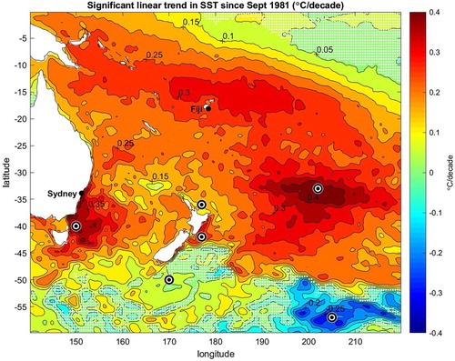
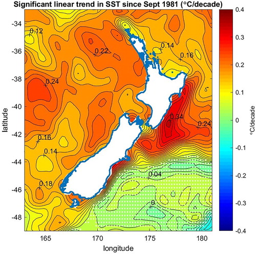
The warming trends are generally weaker but still statistically significant closer to New Zealand (Figure 2), with eastern Tasman warming of ∼0.1–0.3°C/decade. There is very weak warming along the northeast coast of the North Island north of East Cape, which is consistent with the lack of trend detected in the recent analyses of the University of Auckland Leigh coastal SST time series by Shears and Bowen (2017) and Bowen et al. (2017). The strongest warming along the New Zealand coastline occurs on the east coast of the North Island south of East Cape.

Figure 2. As for Figure 1, but focusing on the New Zealand region. Contour intervals are 0.02°C/decade.

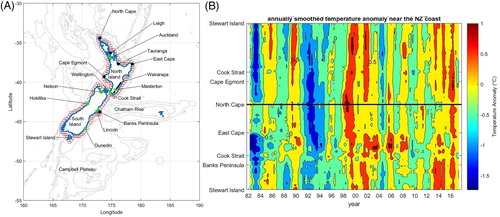
Figure 3 focuses further on changes near the coast. Pixels close to the coast were selected (Figure 3A) and annually-smoothed temperature anomaly timeseries from these locations are shown in Figure 3B with the coastline ‘unwrapped’ so that the y axis begins with Stewart Island before running northward up the east coast to North Cape and then southward along the west coast to complete the circuit at Stewart Island. Correlation length scales implicit in the daily OI-SST product are of the order of 100–150 km (Reynolds et al 2007) or about half the distance between Banks Peninsula and Cook Strait, meaning that Figure 3B is effectively smoothed over this length scale. The OI-SST correlation time scales are much shorter than the annual smoothing and so will not impact Figure 3B. Strong coherence over the entire coastline is clear in Figure 3B, consistent with the finding of Bowen et al. (2017) that interannual changes are correlated over large areas. The general pattern is that 1982–1983 is relatively cool, with a second cool period occurring in the 1990s. There was strong warming in the later 1990s (e.g. Sutton et al. 2005) with 1998 being the warmest year on record in the New Zealand air temperature seven station record until it was surpassed in 2016 (https://www.niwa.co.nz/our-science/climate/information-and-resources/nz-temp-record/seven-station-series-temperature-data). The banding in Figure 3B indicates significant interannual variability. Within the large-scale pattern of variability, there are subtle changes around the coastline. The section of coast between Cook Strait and East Cape shows more warm events through the 2000s, consistent with it being near the region of strongest trends. Conversely, the coast between East Cape and North Cape was not as cool in 1982–1983 and does not show the warm events between 2001 and 2015, consistent with it being a local minimum in warming (Shears and Bowen 2017). The west coast varies largely in unison, which indicates that the eastern end of the HRXBT section is representative of much of the eastern Tasman.

Figure 3. A, The New Zealand Seven Station locations (green). The locations near the coast selected to build a near-coastal timeseries (red). B, the timeseries of annually-smoothed temperature anomaly near the coast. The y axis begins at the southern-most location south of Stewart Island, then runs north along the east coast to North Cape (shown by the black line) before running south along the west coast.

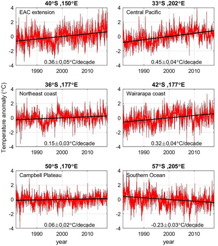
The SST changes at six locations shown in Figure 1 are examined in Figure 4. Daily temperature anomaly timeseries with means and seasons removed indicate variability on all timescales, with the particularly noticeable cool period around New Zealand during the early 1990s followed by rapid warming through the late 1990s (Sutton et al. 2005). The interannual variability and linear trends for each location are also shown. The top two panels show the warming associated with the EAC Extension and central Pacific warming and are the largest trends in the southwest Pacific. In contrast, the strongest warming near the New Zealand coast is the 0.32°C/decade signal east of Wairarapa. There is weak warming off the northeast coast of the North Island, and even weaker on Campbell Plateau. The last panel on the bottom right shows the timeseries from the region with cooling to the southeast of New Zealand. These daily timeseries indicate the changing levels of interannual and decadal variability throughout the region, with the EAC Extension timeseries having the most variability, consistent with its association with the highly-variable EAC and the Campbell Plateau having the least variability.

Figure 4. Daily and annually-smoothed temperature anomalies together with trends for six locations (shown on Figure 1) in the southwest Pacific. Means and seasonal cycles have been removed.

To investigate interannual variability and different regional behaviours, three representative areas around New Zealand were identified from Figures 1 and 2. These are a northeast region, north of the Subtropical Front and east of New Zealand; an eastern Tasman Sea region, north of the Subtropical Front and east of the EAC and a region east of New Zealand and south of the Subtropical Front, largely over Campbell Plateau (Figure 5A). Average daily SST anomalies with means and seasonal cycles removed, along with annually-smoothed (one-year running mean) and linear fits for these three regions are shown in Figure 5B.

Figure 5. A, Three representative areas. B, Spatially-averaged daily SST anomalies for the three regions (with means and seasonal cycles removed), together with annually-smoothed timeseries and linear trends. Daily anomalies more than two standard deviations from the mean are shown in bold.

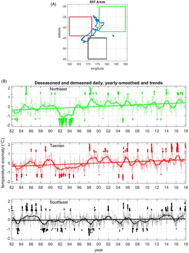
The two subtropical regions (northeast and Tasman) show fairly similar behaviour, are correlated (r = 0.75) and have similar trends (0.22 ± 0.04°C/decade and 0.20 ± 0.03°C/decade, respectively). They both show the cool period through the 1990s, although this cool event was not as pronounced but more persistent in the Tasman. Interannual variability of the order of 1°C is typical, and daily regional-average anomalies tend to be within 2°C of the mean. The southeast timeseries shows somewhat different behaviour, although it is still positively correlated with the subtropical areas (r = 0.28 with the Tasman; r = 0.15 with the northeast). The trend is smaller, at 0.05 ± 0.03°C/decade, there is lower interannual variability of typically ≤0.5°C and lower daily variability of ≤1°C. This relatively low variability is consistent with that seen in the single point Campbell Plateau timeseries in Figure 4.

Extreme events are also indicated in Figure 5, with regionally-averaged temperatures more than two standard deviations from the mean marked in bold. In all regions, the occurrences of warm and cool events are modulated by interannual variability, that is warm extreme events almost exclusively occur during warm periods and cool extreme events during cool periods. This modulation is clear during the early 1990s cool period in subtropical water (the Tasman and northeast regions), particularly so for the northeast, with the bulk of northeast cool events occurring between 1991 and 1995. Beyond this decadal modulation, there is no clear trend in the occurrence of warm or cool events in the northeast or southeast regions. There is the suggestion that the occurrence of warm events in the Tasman region is becoming more frequent, and cool events look to be becoming rarer, with only one Tasman cool event since 2008, as could be expected given the significant warming trend.

• ii) Subsurface (HRXBT) trends

The two repeat HRXBT transects provide the longest timeseries of subsurface temperature in the southwest Pacific. The data locations for the northern (New Zealand to Fiji) transect (PX06) are shown in Figure 6 along with the linear temperature trends as a function of depth between the surface and 850 m (the maximum depth of the XBT) and through the latitude range between New Zealand and Fiji. Areas where the trends are not significant at the 95% level are shaded in white.

Figure 6. A, locations of the XBT casts used in the analysis of ocean temperatures between New Zealand and Fiji from repeat HRXBT line PX06. B, linear trends in temperature between the surface and 850 m along the mean HRXBT track. Regions where the trend is not significant are shaded in white. Contour intervals are 0.05°C/decade.

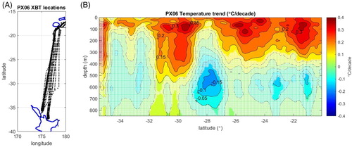
The pattern of change along this northern transect shows an irregular upper layer of significant warming overlaying a layer of almost entirely statistically insignificant cooling. As with the SST analysis, shallow warming trends are small near the New Zealand northeast coast.

The positions of the Tasman HRXBT data are shown in Figure 7 along with the temperature trends. For this transect the position along the transect is demarked by longitude and areas where the trend is not significant are again shaded in white. A reasonable proportion of the western end of the transect does not have significant trends as a result of strong innate variability in the western Tasman associated with the EAC. This high variability impacts the XBT analysis more than the SST analysis because of the shorter record and less frequent sampling of the XBT data. A layer between 100 and 300 m depth east of 164°E also has trends that are not significant. This is a result of longer autocorrelation times of between 1 and 2 years (compared with 0.25 years elsewhere) decreasing the degrees of freedom.

Figure 7. A, locations of the XBT casts used in the analysis of Tasman Sea temperatures from repeat HRXBT line PX34. B, linear trends in temperature between the surface and 850 m along the mean HRXBT track. Regions where the trend is not significant are shaded in white. Contour intervals are 0.05°C/decade.

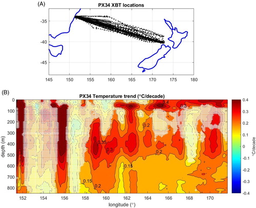
The eastern Tasman is seen to warm significantly in a continuation of the warming through the 1990s discussed by Sutton et al. (2005). There is the suggestion of three layers, 0–100 m which is consistent with winter mixed layer depths, 100–500 m and deeper than 500 m.

• iii) Intercomparison between SST, HRXBT and Argo

The three different observations: satellite SST, HRXBT and Argo can be compared at surface locations along the HRXBT transects. Figure 8 shows SST, 5 m HRXBT and 0–5 m Argo timeseries that have been annually-smoothed with a 12 month running mean, demeaned and deseasoned together with their linear trends for a location north of Auckland along PX06 and a second location in the eastern Tasman along PX34.

Figure 8. Comparison of SST, 5 m HRXBT and 0–5 m Argo timeseries for locations along the northern PX06 transect (A) and the Tasman PX34 transect (B). All timeseries have had means and seasonal cycles subtracted and been annually smoothed with a 12-month running mean filter. The linear trends from each timeseries are also shown.

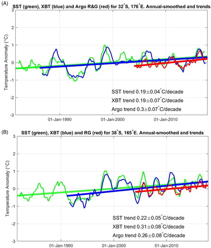
The timeseries are consistent, given the different measurement and mapping techniques: SSTs being objectively-interpolated, twice-daily radiometer-based estimates of the upper ∼0.5 m; HRXBT results being 5 m estimates from harmonically-interpolated, approximately quarterly ocean measurements using a thermistor and Argo being an objective analysis of 0–5 m data from floats spaced every ∼3°latitude/longitude and cycling every 10 days making ocean measurements using a CTD. HRXBT results from the 10 m depth level were almost identical and had the same trends to two decimal places, confirming that near-surface artefacts are not impacting the XBT results. Notable is that the PX34 timeseries was started during a cool period in the Tasman in the early 1990s, which was followed by a period of dramatic warming as discussed by Sutton et al. (2005). As the timeseries has continued, the cool start time has had diminishing impact on the trends, but the HRXBT trend (0.31 ± 0.08 °C/decade) is still higher than the SST trend (0.22 ± 0.05°C/decade) in a salutary lesson about the limitations of short timeseries and the impact of anomalies at the ends of timeseries on calculating trends. In contrast, the HRXBT PX06 transect was started earlier, in 1986, and the trend is not as impacted by the cool conditions around New Zealand in the early 1990s. Indeed, at this location the SST and HRXBT trends are the same at 0.19 ± 0.04 and 0.19 ± 0.07°C/decade.

The consistent trend calculations between the short Argo timeseries and the longer HRXBT and SST timeseries are somewhat serendipitous. Earlier analyses based on slightly shorter periods did not show such good agreement. The Argo dataset is not long enough to robustly estimate decadal trends at high spatial resolution, but is already sufficient to determine decadal trends by spatially averaging to reduce noise (e.g. Roemmich et al. 2015).

• iv) Depth extent of surface changes

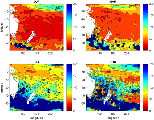
While the Argo timeseries is still too short to calculate significant local trends, the spatial and temporal coverage from Argo allow the relationships between 0–5 m and subsurface temperature variability to be investigated, in particular the correlation between 0–5 m and subsurface temperature changes. This is of interest because it informs the interpretation of changes in the subsurface ocean in relation to the longer, readily-available, high-resolution satellite SST timeseries. Previous studies have shown that 0–5 m Argo measurements are a good representation of SST, with Roemmich and Gilson (2009) comparing the topmost depth of their Argo climatology with OI-SST and finding the variance of the difference to be ∼0.04 (°C)² and Roemmich et al. (2015) finding that the global mean Argo temperature above 5 m tracks closely with SST change. Figure 9 shows the depths at which the correlation with surface temperature changes drops to 0.7 for the four seasons based on monthly 1°latitude/longitude, objectively-analysed data from the Roemmich and Gilson Argo climatology (Roemmich and Gilson 2009). It was chosen to do this analysis on a seasonal basis because the seasonal cycle of the upper ocean with the formation and decay of the mixed layer could be expected to determine the upper ocean vertical length scales. Indeed, this is the case. Summer (DJF) sees the smallest r = 0.7 correlation depths (∼40 m), with deepening through autumn (MAM). The winter and spring seasons see this correlation depth extending to more than 100 m around most of New Zealand, meaning that changes in SST of spatial scales of the order of 1°latitude/longitude and time scales of the order of a month are correlated (r = 0.7) with temperature changes down to more than 100 m. The area associated with the Subantarctic Front (SAF) south of New Zealand shows correlations to large depths, apparent across a small area in summer expanding to a large area in winter. This is consistent with the low stratification and very deep winter mixed layers associated with this region. Winter in this region saw the ocean down to 2000 m (the maximum Argo depth) still correlated with the surface changes (at r = 0.7).

1. Relationship with New Zealand air temperature

Figure 9. Depth at which the correlation with the surface falls to 0.7 for deseasoned, seasonal data. Based on Argo (RG climatology). Contours are at 20 m intervals.

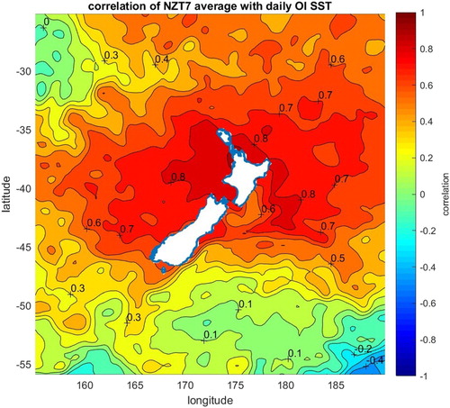
Also of interest is the relationship between New Zealand terrestrial air temperature and SST. This was investigated using the New Zealand Seven Station air temperature series (7SS). The 7SS is calculated by subtracting the 1981–2010 temperature averaged over seven stations (Auckland, Masterton, Wellington, Nelson, Hokitika, Lincoln, and Dunedin) from the monthly averages of the seven stations (Folland and Salinger 1995; Mullan et al. 2010). The 7SS timeseries have been corrected for measurement site relocations and instrument changes to provide consistent measurements of air temperatures at 7 sites across New Zealand. Here, we correlated annual anomalies of the mean 7SS temperature with annual mean SST anomalies calculated from the OI-SST product (Figure 10). The results indicate a large area of significant correlation between air temperatures and SST for interannual timescales, with the highest correlations in the eastern Tasman Sea west of the North Island. Correlations decrease west of 160°E and south of around 45°S. The large area of high correlation is consistent with the analysis of Bowen et al. (2017) who found significant correlations between the coastal SST measurements made at Leigh, north of Auckland and a similarly large area on interannual timescales.

Figure 10. Correlation of annual-average SST with mean of terrestrial New Zealand Seven Station record (annually-averaged).

The trends and 95% confidence intervals for the individual 7SS stations and their mean were also calculated for the period since 1981 coincident with the OI-SST product. The individual station trends were: Auckland: 0.20 ± 0.15°C/decade; Masterton: 0.04 ± 0.18°C/decade; Wellington: 0.06 ± 0.16°C/decade; Hokitika: 0.11 ± 0.17°C/decade; Nelson: 0.23 ± 0.15°C/decade; Lincoln 0.11 ± 0.15°C/decade; Dunedin: 0.09 ± 0.15°C/decade; with the mean NZT7 trend since 1981 being 0.12 ± 0.15° C/decade.

Discussion

Analysis of the nearly 40-year timeseries of SST reveals that SST has warmed over most of the southwest Pacific. However, different regions show different warming rates. The results show significant warming over much of the ocean north of the Subtropical Front (STF), with no warming or slight cooling south of the STF (Figures 1–5). There is weaker warming in the tropics northeast of New Zealand, and cooling in the Southern Ocean east of New Zealand.

Over the wider region, there are two localised areas with high warming rates. The first is off the east coast of Australia in the southernmost extent of the EAC and the EAC Extension. This strong warming is consistent with the global observations of strongest warming in the western boundary currents of the five subtropical gyres (Wu et al. 2012). The temperature increase in this region has been noted by numerous earlier studies as a global ‘hotspot’ with warming 3–4 times greater than the global average due to changes in the EAC and the EAC Extension extending further south in recent decades (e.g. Ridgway 2007; Hill et al. 2008).

The second area of strong warming is in the central South Pacific gyre centred on ∼ 160°E, 35°S. This central Pacific signal has also been described in earlier studies, with Roemmich et al. (2007) and Roemmich et al. (2016) identifying the manifestation of this signal in sea surface height. Both the EAC Extension and central Pacific warming maxima have been attributed to a spin-up of the subtropical gyre due to increased winds (Ridgway 2007; Roemmich et al. 2007; Wu et al. 2012; Roemmich et al. 2016).

Adjacent to New Zealand, the strongest warming occurs along the east coast of the North Island south of East Cape. This is the southernmost limit of the local western boundary current (WBC), the East Cape Current, and so this localised warming maximum is analogous to the warming off the southeast coast of Australia. However, while much of the warming signal in the EAC and EAC Extension regions results from boundary current changes with the EAC Extension strengthening and moving south, the separation of the WBC from the New Zealand coast is geographically locked by Chatham Rise bathymetry (e.g. Chiswell et al. 2015). Furthermore, in their study of variability in New Zealand boundary currents, Fernandez et al. (2018) found no discernable trend in East Cape Current transport. Therefore, the underlying reason for this localised signal remains a matter for further research. The weakest warming around New Zealand occurs along the northeast coast of the North Island, concurring with the results of Shears and Bowen (2017) who found no significant trend in a longer timeseries of coastal SST measured at Leigh, north of Auckland. The difference in signals north and south of East Cape is counter to a conventional paradigm that the East Cape Current is largely a continuation of the East Auckland Current, which would indicate that the two regions are strongly coupled. However, Fernandez et al. (2018) found little coherence between the East Cape and East Auckland Currents, consistent with the different SST trends found here.

The regional variability in warming trends indicates that environmental and ecological impacts could vary spatially, with the strongest trend in the region between East Cape and Cook Strait and the significant trend in the already warm north west coast suggesting those areas are most vulnerable to impacts.

The nearly 40 years of warming in subtropical waters since 1981 at approximately 0.12–0.34°C/decade (Figure 2) is of similar magnitude to future regional warming predicted by earth system models. Law et al. (2017) indicated mid-century warming rates of 0.2 and 0.25°C/decade for moderate (RCP4.5) and high emissions (RCP8.5) projections. These projections indicating surface warming trends of 0.14 and 0.31°C/decade respectively for the end-of-century 2100.

Subsurface trends around New Zealand over the past few decades show temperature increases in the upper few hundred metres around the country (Figures 6 and 7) with increases extending to 850 m in the Tasman Sea (Figure 7). Both HRXBT lines show significant warming through the biologically-significant euphotic zone. From the Argo time series, the changes at the surface can be correlated with the changes at depth to infer the depth of temperature anomalies reflected by the longer time series of surface temperature. Around New Zealand, this ranges from ∼40 m in summer down to 100 m or more in winter. South of New Zealand near the Subantarctic Front, surface variability is correlated to great depths (>1000 m), consistent with the weak stratification and deep mixed layers found in this region. This coupling between the surface and deeper ocean is also a likely contributor to the lower SST trends found to the south, with Southern Ocean heat content changes being spread over a much thicker layer than those to the north. The vertical correlations calculated from the Argo product and the agreement between the SST, HRXBT and Argo analyses where they overlap indicate that the warming trends and seasonal to interannual variability apparent in the SST analysis are likely to persist to at least 40–100 m depth around New Zealand.

The HRXBT transects can also be used to examine the changes in stratification because temperature dominates stratification in the South Pacific. A regularly-cited likely outcome of climate change is increased stratification resulting from upper ocean warming (e.g. Levitus et al. 2009; Rhein et al. 2013). The HRXBT analyses indicate the temperature difference between the surface and 200 m in the eastern Tasman (165°E to 172°E) has increased at a barely-significant rate of ∼0.10 ± 0.08°C/decade. In contrast, for the northern HRXBT P06 transect, the temperature difference between the surface and 200 m south of 30°S has decreased, i.e. the temperature stratification has decreased by –0.11 ± 0.08°C/decade. These trends in upper ocean thermal stratification compare with the global average of ∼0.25°C between 1971 and 2010 (Rhein et al. 2013) or 0.06°C/decade. Calculations of the mixed layer depths from the raw and harmonically-analysed HRXBT timeseries give no indication of changes in mixed layer depths along either of the HRXBT transects. This lack of signals in mixed layer depth could be a result of the quasi-quarterly HRXBT sampling being inadequate to accurately resolve the annual cycle in mixed layer evolution.

New Zealand air temperatures are highly correlated with ocean temperatures over a large area around the country (Figure 10). Similar relationships have been noted in previous studies (e.g. Sutton et al. 2005; Bowen et al. 2017). We find the mean NIWA 7 station air temperature is most strongly correlated with ocean temperatures in the eastern Tasman, as could be expected given the prevailing westerly winds in the New Zealand region. The region of high correlation is largely limited to subtropical water (i.e. north of the STF), coinciding with the region of significant warming. The correlation falls off in the western Tasman but does extend past the dateline to the west.

The mean SS7 air temperature trend (0.12°C/decade) is similar to that found in the eastern Tasman Sea, but the variability between stations indicates significant local variations. Interestingly, Masterton and Wellington have the smallest trends despite their relative proximity to the highest coastal SST trend off the Wairarapa coast. That is likely possible because of the relative rarity of easterly winds and Masterton’s inland location. However, these differences in trend are small compared to the large interannual variability and considering the broad confidence intervals on the 7SS temperature trends.

The nearly 40 years of temperature observations show that interannual and decadal variability dominate the record and their influence on the calculation of trends cannot be neglected. The strongest interannual variability in the New Zealand region is due to the El Niño/Southern Oscillation (ENSO) (e.g. Greig et al. 1988; Folland and Salinger 1995; Sutton and Roemmich 2001; Bowen et al. 2017). The interannual variability is instrumental in determining extreme warm and cold events (Figure 5) and should be expected to do so into the future.

In summary, there has been significant warming over much of the southwest Pacific north of the Subtropical Front since 1981. There are specific regions of stronger warming associated with the EAC and EAC Extension and a region in the central South Pacific gyre – both as a result of gyre spin up. All of the ocean adjacent to New Zealand has warmed, with the strongest warming occurring off the Wairarapa Coast and the weakest along the northeast coast between East Cape and North Cape. The HRXBT transects reveal that the ocean is warming over the upper 200 m around New Zealand and down to 850 m in the Tasman Sea. New Zealand air temperature changes on interannual timescales are highly correlated with a large area of ocean from the eastern Tasman to beyond the dateline, largely over ocean north of the Subtropical Front. Both warm and cool extreme events are modulated by interannual variability. Five year running means of the number of days with warm and cold extremes suggest an increase in the frequency of warm events and decrease in frequency of cool events in the eastern Tasman, but no changes in the other regions.

Acknowledgements

This work was supported by the Deep South National Science Challenge and NZ Ministry of Business, Innovation and Employment (MBIE) NIWA Strategic Investment Funding CAOC1804. NOAA High Resolution SST data were produced by NOAA/NCEI (https://www.ncdc.noaa.gov/oisst) and provided from the NOAA/OAR/ESRL PSD, Boulder, Colorado, USA, website (http://www.esrl.noaa.gov/psd/). HRXBT data were made available by the Scripps High Resolution XBT program (www-hrx.ucsd.edu). The Argo data were collected and made freely available by the International Argo Program and the national programs that contribute to it (http://www.argo.ucsd.edu, http://argo.jcommops.org). The Argo Program is part of the Global Ocean Observing System. The Roemmich and Gilson Argo climatology was accessed from http://sio-argo.ucsd.edu/RG_Climatology.html; http://doi.org/10.17882/42182.

Disclosure statement

No potential conflict of interest was reported by the authors.

Additional information

Funding

The project was partially supported by the Deep South National Science Challenge (https://www.deepsouthchallenge.co.nz/). The science challenges are administered by the Ministry for Business, Innovation and Employment (MBIE) (https://www.mbie.govt.nz/science-and-technology/science-and-innovation/funding-information-and-opportunities/investment-funds/national-science-challenges/).

References

- Banzon V, Smith TM, Chin TM, Liu C, Hankins W. 2016. A long-term record of blended satellite and in situ sea-surface temperature for climate monitoring, modeling and environmental studies. Earth System Science Data. 8:165–176. doi:10.5194/essd-8-165-2016.
- Bartlett MS. 1935. Some aspects of the time-correlation problem in regard to tests of significance. Journal of the Royal Statistical Society. 98:536–543. doi: 10.2307/2342284
- Bowen M, Markham J, Sutton P, Zhang X, Wu Q, Shears N, Fernandez D. 2017. Interannual variability of sea surface temperatures in the Southwest Pacific and the role of ocean dynamics. Journal of Climate. 30:7481–7492. doi:10.1175/JCLID-16-0852.1 doi: 10.1175/JCLI-D-16-0852.1
- Cheng L, Zhu J, Cowley R, Boyer T, Wijffels S. 2014. Time, probe type, and temperature variable bias corrections to historical expendable bathythermograph observations. Journal of Atmospheric and Oceanic Technology. 31:1793–1825. doi:10.1175/JTECH-D-13-00197.1.
- Chiswell S, Grant B. 2018. New Zealand coastal sea surface temperature. NIWA report prepared for the NZ Ministry for the Environment.
- Chiswell SM, Bostock HC, Sutton PJH, Williams MJM. 2015. Physical oceanography of the deep seas around New Zealand: a review. New Zealand Journal of Marine and Freshwater Research. doi:10.1080/00288330.2014.992918.
- Cowley R, Wijffels S, Cheng L, Boyer T, Kizu S. 2013. Biases in expendable bathythermograph data: a new view based on historical side-by-side comparisons. Journal of Atmospheric and Oceanic Technology. 30:1195–1225. doi:10.1175/JTECH-D-12-00127.1.
- Georgi DT, Dean JP, Chase JA. 1980. Temperature calibration of expendable bathythermographs. Ocean Engineering. 7:491–499. doi: 10.1016/0029-8018(80)90048-7
- Fernandez D, Bowen M, Sutton P. 2018. Variability, coherence and forcing mechanisms in the New Zealand ocean boundary currents. Progress in Oceanography. 165:168–188. doi:10.1016/j.pocean.2018.06.002.
- Folland CK, Salinger MJ. 1995. Surface temperature trends and variations in New Zealand and the surrounding ocean, 1871–1993. International Journal of Climatology. 15:1195–1218. doi:10.1002/joc.3370151103.
- Greig MJ, Ridgway NM, Shakespeare BS. 1988. Sea surface temperature variations at coastal sites around New Zealand. New Zealand Journal of Marine and Freshwater Research. 22:391–400. doi: 10.1080/00288330.1988.9516310
- Hanawa K, Rual P, Bailey RJ, Sy A, Szabados M. 1995. A new depth-time equation for Sippican or TSK T-7, T-6 and T-4 expendable bathythermographs (XBT). Deep Sea Research Part I: Oceanographic Research Papers. 42:1423–1451. doi: 10.1016/0967-0637(95)97154-Z
- Hill KL, Rintoul SR, Coleman R, Ridgway KR. 2008. Wind forced low frequency variability of the East Australian Current. Geophysical Research Letters. 35:L08602. doi:10.1029/2007GL032912.
- Hoegh-Guldberg O, Cai R, Poloczanska ES, Brewer PG, Sundby S, Hilmi K, Fabry VJ, Jung S. 2014. The ocean. In: Barros VR., Field CB, Dokken DJ, Mastrandrea MD, Mach KJ, Bilir TE, Chatterjee M, Ebi KL, Estrada YO, Genova RC, Girma B, Kissel ES, Levy AN, MacCracken S, Mastrandrea PR, White LL, editors. Climate change 2014: impacts, Adaptation, and Vulnerability. part B: regional Aspects. Contribution of Working Group II to the Fifth assessment report of the intergovernmental panel on climate change. Cambridge, United Kingdom and New York, NY, USA: Cambridge University Press; p. 1655–1731.
- Johnson CR, Banks SC, Barrett NS, Cazassus F, Dunstan PK, Edgar GJ, Frusher SD, Gardner C, Haddon M, Helidoniotis F, et al. 2011. Climate change cascades: shifts in oceanography, species' ranges and subtidal marine community dynamics in eastern Tasmania. Journal of Experimental Marine Biology and Ecology. 400:17–32. https://doi.org/10.1016/j.jembe.2011.02.032.
- Law CS, Rickard GJ, Mikaloff-Fletcher SE, Pinkerton MH, Behrens E, Chiswell SM, Currie K. 2017. Climate change projections for the surface ocean around New Zealand. New Zealand Journal of Marine and Freshwater Research. doi:10.1080/00288330.2017.1390772.
- Levitus S, Antonov JI, Boyer TP, Locarnini RA, Garcia HE, Mishonov AV. 2009. Global ocean heat content 1955–2008 in light of recently revealed instrumentation problems. Geophysical Research Letters. 36:L07608.
- Mitchell JM Jr., Dzerdzeevskii B, Flohn H, Hofmeyr WL, Lamb HH, Rao KN, Wallén CC. 1966. Climatic Change Technical Note 79, 79pp., World Meteorological Organisation, Geneva.
- Mullan AB, Stuart SJ, Hadfield MG, Smith MJ. 2010. Report on the review of NIWA’s ‘Seven-Station’ temperature series. Tech. Rep. NIWA Information Series 78, 175 pp.
- Pinkerton MH. 2017. Impacts of climate change on New Zealand fisheries and aquaculture. In: Phillips BF, Pérez-Ramírez M, editors. The impacts of climate change on fisheries and aquaculture: a global analysis. 1st ed. John Wiley & Sons Ltd; p. 91–118.
- Reynolds RW, Smith TM, Liu C, Chelton DB, Casey KS, Schlax MG. 2007. Daily high-resolution-blended analyses for sea surface temperature. Journal of Climate. 20:5473–5496. https://doi.org/10.1175/2007JCLI1824.1.
- Rhein M, Rintoul SR, Aoki S, Campos E, Chambers D, Feely RA, Gulev S, Johnson GC, Josey SA, Kostianoy A, et al. 2013. Observations: ocean. In: Stocker TF, Qin D, Plattner G-K, Tignor M, Allen SK, Boschung J, Nauels A, Xia Y, Bex V, Midgley PM, editors. Climate change 2013: The physical science basis. Contribution of Working Group I to the Fifth assessment report of the intergovernmental panel on climate change. Cambridge (UK): Cambridge University Press; p. 255–315.
- Ridgway K, Hill K. 2012. East Australian Current. In: Poloczanska ES, Hobday AJ, Richardson AJ, editors. A marine climate change impacts and adaptation report Card for Australia 2012. <http://www.oceanclimatechange.org.au>; p. 47–60.
- Ridgway KR. 2007. Long-term trend and decadal variability of the southward penetration of the East Australian Current. Geophysical Research Letters. 34:L13613. doi:10.1029/ 2007GL030393.
- Roemmich D, Boebel O, Freeland H, King B, Le Traon P-Y, Molinari B, Owens WB, Riser S, Send U, Takeuchi K, et al. 1998. On the design and implementation of Argo: an initial plan for a global array of profiling floats. International CLIVAR Project Office Report 21, GODAE Report 5. GODAE International Project Office, Melbourne, Australia, 32 pp.
- Roemmich D, Church J, Gilson J, Monselesan D, Sutton P, Wijffels S. 2015. Unabated planetary warming and its ocean structure since 2006. Nature Climate Change. 5:240–245. doi:10.1038/NCLIMATE2513.
- Roemmich D, Cornuelle B. 1990. Observing the fluctuations of gyre-scale ocean circulation: a study of the subtropical South Pacific. Journal of Physical Oceanography. 20:1919–1934. doi: 10.1175/1520-0485(1990)020<1919:OTFOGS>2.0.CO;2
- Roemmich D, Gilson J. 2009. The 2004–2008 mean and annual cycle of temperature, salinity, and steric height in the global ocean from the Argo Program. Progress in Oceanography. 82(2):81–100. https://doi.org/10.1016/j.pocean.2009.03.004.
- Roemmich D, Gilson J, Davis R, Sutton P, Wijffels S, Riser S. 2007. Decadal spin-up of the South Pacific subtropical gyre. Journal of Physical Oceanography. 37:162–173. doi: 10.1175/JPO3004.1
- Roemmich D, Gilson J, Sutton P, Zilberman N. 2016. Multidecadal change of the South Pacific gyre Circulation. Journal of Physical Oceanography. 46:1871–1883. doi:10.1175/JPO-D-15_0237.1 doi: 10.1175/JPO-D-15-0237.1
- Roemmich DH. 1983. Optimal estimation of hydrographic station data and derived fields. Journal of Physical Oceanography. 13:1544–1549. doi: 10.1175/1520-0485(1983)013<1544:OEOHSD>2.0.CO;2
- Santer BD, Wigley TML, Boyle JS, Gaffen DJ, Hnilo JJ, Nychka D, Parker DE, Taylor KE. 2000. Statistical significance of trends and trend differences in layer-average atmospheric temperature time series. Journal of Geophysical Research: Atmospheres. 105(D6):7337–7356. doi: 10.1029/1999JD901105
- Schiel DR. 2013. The other 93%: trophic cascades, stressors and managing coastlines in non-marine protected areas. New Zealand Journal of Marine and Freshwater Research. 47(3):374–391. doi:10.1080/00288330.2013.810161.
- Schiel DR, Lilley SA, South PM, Coggins JHJ. 2016. Decadal changes in sea surface temperature, wave forces and intertidal structure in New Zealand. Marine Ecology Progress Series. 548:77–95. doi:10.3354/meps11671.
- Shears NT, Bowen MM. 2017. Half a century of coastal temperature records reveal complex warming trends in boundary currents. Scientific reports. 7:14527. doi:10.1038/s41598-017-14944-2.
- Sutton PJH, Bowen M, Roemmich D. 2005. Decadal temperature changes in the Tasman Sea. New Zealand Journal of Marine and Freshwater Research. 39:1321–1329. doi: 10.1080/00288330.2005.9517396
- Sutton PJH, Roemmich D. 2001. Ocean temperature climate off north-east New Zealand. New Zealand Journal of Marine and Freshwater Research. 35:553–565. doi: 10.1080/00288330.2001.9517022
- Wu L, Cai W, Zhang L, Nakamura H, Timmermann A, Joyce T, McPhaden MJ, Alexander M, Qiu B, Visbeck M, et al. 2012. Enhanced warming over the global subtropical western boundary currents. Nature Climate Change. doi:10.1038/nclimate1353.