New Zealand estuary benthic health indicators summarised nationally and by estuary type

ABSTRACT

Ecological data are often collected at small geographic scales. However, analysing data collectively over wider scales can reveal results and patterns not shown in the smaller-scale data. We summarised data for intertidal benthic ecological (physico-chemical and biological) health indicators from New Zealand estuaries and compared the results against thresholds above which ecological impacts are expected to occur. Values for the sediment physico-chemical indicators mud and nutrients (nitrogen and phosphorus collectively) were above thresholds for at least 50% and at 31% of sites measured respectively. Sediment organic content and metal concentrations were generally low, with only maximum values exceeding the thresholds. Scores for biological indicators were within (or better than) the moderate health category for either at least 50%, or at least 75%, of sites. When compared across estuary types (based on a geomorphic classification system) we found statistically significant differences for thirteen of the sixteen indicators. Differences (among mean values) for highly significant results were relatively large compared to the range of values observed nationally for those indicators. However, the differences, except those for mud, were smaller than their respective ecological health threshold values. Our summary provides a reference for future comparisons of estuary indicators nationally and across estuary types.

KEYWORDS:

• Estuary
• classification
• type
• biotic index
• indicator
• health

Introduction

Estuaries connect terrestrial, freshwater and marine environments and perform essential ecological functions (Levin et al. 2001). They also deliver valuable ecosystem services (Costanza et al. 1997) and are the focus of intense human activity (Ewel et al. 2001; Edgar and Barrett 2002). Growing human populations and intensifying land-use practices are increasing negative stresses on estuaries and compromising their environmental health (Lotze et al. 2006; Ellis et al. 2015).

Ecological indicators provide information about the health of ecosystems (Cairns et al. 1993). Indicators associated with benthic sediments are commonly used for monitoring in estuaries as these habitats are functionally important (Borja et al. 2015), can act as sinks for contaminants (Kennish 1997), and are relatively stable over time (i.e. less variable than the overlying water column) (Salas et al. 2006). The dynamics of sediment habitats can also be closely related to processes happening in the overlying water (Magni 2003). For example, sediment physico-chemical variables and the composition and condition of sediment-dwelling macroinvertebrate communities have been quantitatively linked to seawater variables such as dissolved oxygen and those associated with eutrophication (Dauer et al. 2000; Eyre and Ferguson 2006; Dimitriou et al. 2015). A combination of indicators is often used to assess estuary benthic health (Borja et al. 2008; O’Brien et al. 2016). Biotic indices measure the response of macrofaunal communities to environmental change (Weisberg et al. 1997; Borja et al. 2000). Physico-chemical variables, often those influenced by human activities, are also commonly used as benthic health indicators (Birch and Olmos 2008; Van Niekerk et al. 2013).

The monitoring and reporting of estuary environmental condition is considered essential for managing these ecosystems (Hallett et al. 2016). Effective monitoring can help prioritise and evaluate environmental policy, as well as advance environmental knowledge (Lovett et al. 2007). Environmental data are commonly reported at small (e.g. sub-national or local) geographic scales (Lovett et al. 2007), with wider-scale reporting (e.g. national) often impeded by inconsistencies between local datasets (GAO 2002; Hughes and Peck 2008; Ellingsen et al. 2017). However, assessing and reporting environmental health data collectively (e.g. Heinz Center 2002; Kristensen et al. 2013) enables results and patterns from smaller scale data to be placed within a larger (e.g. national or international) context (Magni 2003; Van Niekerk et al. 2013; Schiff et al. 2016).

Estuaries vary in their physical properties (i.e. exhibit abiotic variation) and can be classified into types accordingly (Engle and Summers 1999; Bald et al. 2005; Hume et al. 2007). These abiotic differences can help explain estuarine processes and patterns at large scales (Hume et al. 2007). For example, biological characteristics of estuaries, such as the composition of animal and plant communities, can be associated with estuarine hydrological and morphological characteristics (Saintilan 2004; Galván et al. 2010; Lucena-Moya and Duggan 2017). Being able to compare data across estuary types is one benefit of wider scale reporting, and differences in benthic ecological health indicators have been observed across estuary types (Edgar et al. 1999; Muxika et al. 2007; Barbone et al. 2012). Identifying natural differences across estuary types may be important for setting management targets, while knowledge of differences caused by human impacts can also guide estuary management decisions. A first step for identifying ecological differences across estuary types can be to explore these differences irrespective of whether those that are natural or anthropogenic in origin are quantified separately.

New Zealand sits within the biogeographic realm of temperate Australasia (Spalding et al. 2007). It contains approximately 440 estuaries that, due to the country’s diverse oceanography, climate, landforms and geology, belong to a variety of estuary types (Hume and Herdendorf 1988; Hume et al. 2007). Threats identified for New Zealand’s coastal environment include sedimentation, excess nutrients, organic enrichment and metal contamination (MFE & StatsNZ 2016; Robertson et al. 2016), all of which occur naturally but are exacerbated by human pressures. Although intertidal benthic ecological (physico-chemical and biological) health indicator data have been collected in estuaries throughout New Zealand, they have generally not been summarised and reported on a scale that enables national comparison (although see MFE & StatsNZ (2016)). They have also not been comprehensively compared across New Zealand’s estuary types (for smaller scale studies see Thrush et al. 2003; Ellis et al. 2006; de Juan et al. 2013; Berthelsen, Atalah, et al. 2018).

To enable national comparisons of estuary health, we used data collected from fourteen New Zealand regions to summarise intertidal benthic ecological (physico-chemical and biological) health indicators nationally, as well as compare them against thresholds above which ecological impacts are expected to occur. In addition, we compared benthic indicators across estuary types grouped using a geomorphic classification system.

Methods

Data

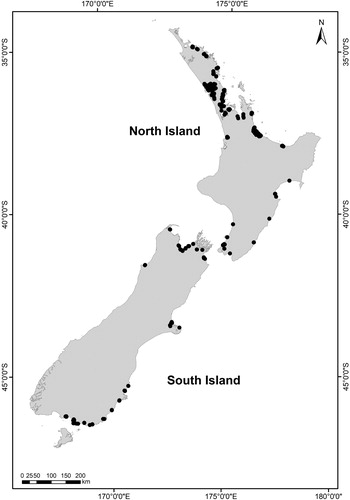
Benthic macrofauna and matching sediment physico-chemical health indicator data were collected from intertidal estuary sites by fourteen of New Zealand’s local government authorities; we combined these with data from other research programmes. Survey dates ranged from 2001 to 2017, generally between September and May. Sixty estuaries (14% of New Zealand’s estuaries) containing 347 sites were represented in the data (Figure 1). The number of sites per estuary (range 1–50), the number and type of indicators surveyed per site and the survey years, depended on estuary size and/or the regional or research sampling regime. Sites were located on unvegetated soft sediments at mid-low tidal height and generally away from the direct influence of point source discharges. Surveys were conducted as per a standardised protocol (Robertson et al. 2002) with some minor variations (e.g. site size, number of replicates collected). Sample collection methods are described in Berthelsen, Clark, et al. (2018).

Figure 1. The location of New Zealand estuaries (and sites) from where intertidal benthic ecological (physico-chemical and biological) health indicator data in this study were obtained.

Estuary classification

We assigned an estuary type to each site using a geomorphic classification system (Hume et al. 2016a, which built on earlier studies such as Hume et al. 2007). More specifically, this system discriminates estuaries by their ‘landscape and waterscape characteristics, such as geology, geomorphology and hydrodynamic characteristics arising from river and oceanic forcing and basin morphometry’ (Hume et al. 2016a). Estuaries in this study were assigned to the following geomorphic classes (GCs): waituna-type lagoon (GC2), tidal river mouth (GC6 subclasses a, b and c combined), tidal lagoon (GC7 subclass a), shallow drowned valley (GC8), deep drowned valley (GC9) and coastal embayment (GC11). Larger estuaries can contain a variety of estuary types within them. We assigned geomorphic classes based on information in the New Zealand Coastal Hydrosystems database (Hume et al. 2016b).

Indicators

The ten benthic physico-chemical health indicators in our study related to grain size, and nutrient and metal concentrations, of benthic sediments (Table 1). Mud was the most commonly sampled physico-chemical indicator (338 sites), and total organic carbon (TOC) the least sampled (81 sites). There were inconsistencies in some analytical methods across the many surveys and laboratories used (Hewitt et al. 2014; Berthelsen, Clark, et al. 2018). Two main methods were used to analyse sediment grain size: wet sieving (majority of data for all estuary types except GC9) and laser diffraction. We standardised grain size (as a percentage of particles < 2 mm). We compared the indictor mud overall (all data combined) across estuary types, however, since the grain size analysis methods can yield different results (Hunt and Jones 2018) we also performed separate comparisons for each analysis method. Most nitrogen data were analysed as total nitrogen (TN) (93%), with the small proportion of data analysed as Total Kjeldahl Nitrogen (hereafter also referred to as TN) spread across all estuary types in our comparative analyses. The analytical detection limit (ADL) was unknown for some data. We therefore designated this based on the highest known ADL for each indicator and assigned all averaged physico-chemical indicator values below their designated ADL a value that was half that of the ADL. The ADL applied to the TN data (500 mg/kg) was relatively high in relation to known ecological thresholds as well as to TN levels present at most sites in our data.

Table 1. Summary of intertidal benthic ecological (physico-chemical and biological) health indicators for soft sediments in New Zealand estuaries (data averaged per site and collected between 2001 and 2017).

Indicator	Minimum	q25	Median	q75	Maximum	Mean	SD	n
Physico-chemical
Mud (% grain size < 63 µm out of < 2 mm)	0.0	4.4	12.4	27.9	99.9	21.6	24.3	338
Total organic carbon (TOC, %)	0.0	0.2	0.4	0.6	3.4	0.6	0.7	81
Total nitrogen (TN, mg/kg) ADL = 500	250.0	250.0	250.0	746.5	3700.0	602.6	569.5	205
Total phosphorus (TP, mg/kg) ADL = 40	53.0	220.0	349.8	520.8	1413.3	393.4	228.0	192
Cadmium (Cd, mg/kg) ADL = 0.1	0.05	0.05	0.05	0.05	1.00	0.06	0.09	177
Chromium (Cr, mg/kg) ADL = 2	2.3	7.0	11.5	20.3	104.3	16.8	15.2	177
Copper (Cu, mg/kg) ADL = 2	1.0	1.0	4.7	8.3	38.0	6.1	6.1	237
Nickel (Ni, mg/kg) ADL = 2	1.0	4.4	7.1	11.6	95.3	11.6	15.5	177
Lead (Pb, mg/kg) ADL = 1	0.5	2.3	4.3	8.0	45.7	6.6	7.1	237
Zinc (Zn, mg/kg) ADL = 7.5	3.8	18.0	33.0	50.0	236.7	41.2	33.7	237
Biological
Richness-integrated AMBI (RI-AMBI)	1.0	1.7	1.9	2.3	3.6	2.0	0.5	316
Traits based index (TBI)	0.01	0.22	0.32	0.42	0.73	0.32	0.14	342
Metals benthic health model (MetalsBHM)	1.0	2.5	3.4	3.9	5.9	3.2	1.0	98
Mud benthic health model (MudBHM)	0.5	2.9	3.6	4.5	5.3	3.6	1.0	167
N (individuals per 0.0133 m^2)	6.3	48.3	87.2	141.7	1259.0	115.8	114.8	316
S (taxa per 0.0133 m^2)	3.1	6.3	9.8	14.0	25.2	10.4	4.7	316

Values below the designated analytical detection limits (ADL) are shown as half of the ADL (indicated by grey cells). Abbreviations include q25 and q75 for the 25th and 75th percentiles respectively, SD for standard deviation and n for the number of sites represented in the data.

The biological health indicators comprised four biotic indices recently identified as potential candidates for nationwide monitoring in New Zealand estuaries (Berthelsen, Atalah, et al. 2018; Clark et al. in prep): the richness-integrated AZTI marine biotic index (RI-AMBI), traits based index (TBI) and two benthic health models (MudBHM and MetalsBHM) (Table 1). Two simple metrics (total abundance (N) and total number of taxa (S)) were also calculated.

Prior to biotic index/metric calculation (for RI-AMBI, TBI, S and N), processing of the macrofaunal data involved taxonomic lumping and scaling of abundance based on core diameter (as described by Berthelsen, Atalah, et al. 2018), as well as removal of some taxa and data (sites with S < 3 and/or N < 3) (Borja and Muxika 2005). RI-AMBI scores were calculated following Robertson et al. (2016), for sites where > 80% of taxa were assigned to ecogroups (Borja and Muxika 2005). Ecogroups were derived from information sources prioritised in the following order: Robertson et al. (2015), Keeley et al. (2012) and AZTI (2018). The TBI scores were calculated using site-averaged data generally following Rodil et al. (2013). Data preparation and index calculation for the two multivariate BHMs (MudBHM and MetalsBHM) are detailed in Clark et al. (in prep), with index scores only calculated for sites with sufficient taxonomic resolution.

The level of taxonomic resolution at which macrofaunal taxa are identified can influence biotic index scores (Dauvin et al. 2003; Trigal-Domínguez et al. 2010). We tested a subset of our data against high resolution data from corresponding sites. Besides suppressing values for S (as expected), taxonomic lumping resulted in index scores that were generally slightly lower for RI-AMBI (resulting in healthier scores) and TBI (resulting in unhealthier scores) than those derived from the high-resolution data. Although this will have had a slight (although larger for S) influence on our summary scores, correlations were high between indices calculated from both high- and low- resolution data, giving us confidence that the taxonomic lumping will not affect the results of our comparative analyses.

Indicator data were averaged at site level and only the most recent data available for each indicator at each site was included in the analyses. The analysed data were largely (89%) from 2010 to 2017, with the oldest data from 2001. Although older data could be less reflective of current conditions, we chose to retain all sites in our analyses rather than exclude them based on an arbitrary date cut-off. Depending on when each indicator was last sampled at a site, indicator data from different years may have been used from the same site.

Indicator summary

Indicators were summarised using basic descriptive statistics overall (i.e. nationally). Ecological health in the context of our study was interpreted separately for each indicator (although nutrients were also considered together) in relation to the physico-chemical variable it represented. Some indicators (i.e. biotic indices) measured a response to a physico-chemical variable or combination of these. To guide interpretation of indicator health, we compared indicator summary values against ecological thresholds above which negative ecological effects are expected (Table 2). The thresholds provided a guide only as they were largely derived from research papers or reports, rather than being government-adopted guidelines. Also, some thresholds had been validated for a certain area (or estuary type) only although we applied them all nationally. For the metals, we used the more conservative Environmental Response Criteria (ERC) (ARC 2004), although used the Australian and New Zealand Environmental and Conservation Council default guideline values (DGVs) (ANZECC & ARMCANZ 2018) when ERCs were not available. The thresholds were generally comparable to our results, although we did not make a detailed assessment of the laboratory analytical methods for data used to derive them. We largely limited our interpretation of results to the median, 75th percentile and maximum values, as these reflect general patterns nationally and the unhealthiest sites respectively. Although lower values are also of interest, these were usually below ecological thresholds (25^th percentile) and the ADL (minimum), and so were of limited usefulness to our interpretations. We also calculated Pearson’s correlations between indicators, with high correlation strength defined as r ≥ |0.8| (Jun et al. 2012).

Table 2. Benthic sediment physico-chemical and biological indicator thresholds for ecological health in New Zealand estuaries.

Indicator	Ecological threshold	Description	Relevant region	Reference
Mud	<5%	Estimated optimum for the three most sensitive macrofaunal taxa (from 20 taxa).	Auckland region estuaries	Anderson (2008)
	5%	Optimum and distribution maximums for the five most sensitive macrofaunal taxa (of 38 taxa).	Auckland region estuaries	Norkko et al. (2002)
	10%	Highest optimum mud value for the 11 most sensitive macrofaunal taxa (of 39 taxa).	New Zealand estuaries	Robertson et al. (2015)
	<10%	Coincided with higher functional redundancy of macrofaunal communities (i.e. TBI scores).	Auckland region estuaries	Rodil et al. (2013)
	18%	Upper optimum level (90th percentile) for 20 macrofaunal taxa.	Tauranga Harbour	Ellis et al. (2017)
	<16%	Upper optimum level (90th percentile) for 22 macrofaunal traits.	Tauranga Harbour	Ellis et al. (2017)
	>25%	Less diverse and less abundant macroinvertebrate communities.	New Zealand estuaries	Robertson et al. (2015)
	2%–30%	Normal to impoverished macrofaunal community.	New Zealand estuaries	Robertson et al. (2016)
Total organic carbon (TOC)	<1%	Low risk of reduced macrobenthic richness.	Worldwide coastal regions	Hyland et al. (2005)
	>3%–4%	‘Transitional to pollution’ to ‘polluted’ macrofaunal community or ‘moderate’ to ‘poor’ ecological status.	New Zealand estuaries	Robertson et al. (2016)
	>3.5%	High risk of reduced macroinfaunal richness.	Worldwide coastal regions	Hyland et al. (2005)
Total nitrogen (TN)	630 mg/kg*	Upper optimum level (90th percentile) for 20 macrofaunal taxa.	Tauranga Harbour	Ellis et al. (2017)
	995 mg/kg*	Upper optimum level (90th percentile) for 22 macrofaunal traits.	Tauranga Harbour	Ellis et al. (2017)
Total phosphorus (TP)	215 mg/kg*	Upper optimum level (90th percentile) for 20 macrofaunal taxa.	Tauranga Harbour	Ellis et al. (2017)
	320 mg/kg*	Upper optimum level (90th percentile) for 22 macrofaunal traits.	Tauranga Harbour	Ellis et al. (2017)
Metals	Cu = 19 mg/kg Pb = 30 mg/kg Zn = 124 mg/kg	Lower threshold for ‘Amber’ environmental response criteria (ERC). The biology of the site is possibly impacted.	Auckland coastal marine area	ARC (2004)
Metals	Cd = 1.5 mg/kg Cr = 80 mg/kg Ni = 21 mg/kg	Default guideline value (DGV) – indicates the concentrations below which there is a low risk of unacceptable effects occurring.	Australia and New Zealand	ANZECC and ARMCANZ (2018)
Richness-integrated AZTI marine biotic index (RI-AMBI) Index range = 1–7	0.0–0.2 = high 0.2–1.2 = good 1.2–3.3 = moderate 3.3–4.3 = poor 5.0–6.0 = bad 6.0–7.0 = azoic	Macrofaunal community response to mud and enrichment gradients.	New Zealand shallow, intertidal dominated estuaries.	Robertson et al. (2016)
Traits based index (TBI) Index range = 1–0	0–0.3 = poor 0.3–0.4 = intermediate 0.4–1 = high	Macrofaunal functional redundancy in response to mud and metal gradients.	Auckland region estuaries.	Rodil et al. (2013)
Mud and metals benthic health models (MudBHM and MetalsBHM) Index range = 1–6	1–2 = 1 (least impacted) 2–3 = 2 3–4 = 3 4–5 = 4 5–6 = 5 (most impacted)	Macrofaunal community response to mud (MudBHM) and metal (MetalsBHM) gradients.	New Zealand tidal lagoon and shallow drowned valley estuaries.	Clark et al. (in prep)

*individual total nitrogen (TN) and total phosphorus (TP) thresholds based on analyses that used a combined nutrient gradient.

Comparisons across estuary types

Differences in indicator values across estuary types were explored using unbalanced one-way ANOVA models. Assumptions regarding normality and homogeneity of variance of the data were met, with transformation conducted if necessary (Zuur et al. 2010). We used Tukey’s test for pairwise comparisons to test specific differences between indicators and estuary types. For all significant pairwise comparisons, we confirmed that the 95% confidence intervals did not cross zero. Due to the unbalanced nature of our data (i.e. varying numbers of sites, and regions represented by sites, per estuary type), we did not include an interaction of region in these analyses. To reduce the likelihood of certain regions or estuaries influencing our results, we excluded estuary types for which fewer than four regions (and fewer than six estuaries) were represented for a given indicator. For mud analysed separately per grain size analysis method, we lowered this minimum to fewer than two regions (and fewer than three estuaries), as separating the data reduced the amount of data available for each analysis. The data excluded were: waituna-type lagoons and coastal embayments (all indicators), tidal river estuaries (mud values derived from laser grain size analysis), deep drowned valley estuaries (TOC), and tidal river and deep drowned valley estuaries (MudBHM and MetalsBHM). Differences across estuary types were considered significant if P < 0.05 and highly significant if P < 0.001 for ANOVAs and pairwise comparisons. Additionally, we considered significant and highly significant ANOVA results as P < 0.003 and P < 0.00006 respectively based on a Bonferroni correction for family-wise error. The total number of estuaries and sites per estuary type in our comparative analyses were: tidal river (7 estuaries, 16 sites), tidal lagoon (24, 124), and shallow (19, 179) and deep (8, 26) drowned valley, although these values varied per indicator (Figure 2).

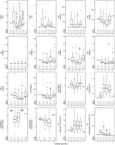
Figure 2. New Zealand intertidal benthic ecological (physico-chemical and biological) health indicators across estuary types classified by geomorphic class (GC); waituna-type lagoon (GC2), tidal river (GC6), tidal lagoon (GC7), shallow (GC8) and deep (GC9) drowned valley, and coastal embayment (GC11) estuaries. The box plot for each indicator displays the median, 25th and 75th percentiles. The number of estuaries (n(e)) and sites (n(s)) are provided under each plot. An asterisk symbol (*) either side of the indicator name on the y-axis shows there was a significant difference (determined using unbalanced one-way ANOVA models, P < 0.05) across at least one estuary type pair for that indicator. Mud is represented by separate box plots (overlaid on each other) for each sediment grain size analysis method (laser (grey box plot) and wet sieving (white box plot)). The number of estuaries and sites for the mud plot represents the combined data (wet sieve and laser).

Results

Indicator summary

Sediment mud content for at least 50% of sites measured (i.e. median = 12.4% mud) was above threshold values (5% and 10% mud) at which sensitive macrofaunal taxa and traits (based on functional redundancy) are expected to be negatively impacted (Tables 1 and 2). Also, the mud content for at least 25% of sites overall (i.e. q75 = 27.9%), including some of those mentioned above, was higher than the threshold (25% mud) where macrofaunal communities are expected to be less diverse and less abundant. The mud q75 value was also above the upper optimum for macrofaunal taxa (18% mud) and traits (16% mud) based on research in Tauranga Harbour.

Total phosphorus (TP) for at least 50% of sites measured (i.e. median = 349.8 mg/kg TP), was above the upper optimums (based on a combined nutrient gradient) for macrofaunal taxa (215 mg/kg TP) and macrofaunal traits (320 mg/kg TP) in Tauranga Harbour (Tables 1 and 2). For total nitrogen (TN), values were below the ADL for at least 50% of sites measured (i.e. median = 250 mg/kg). The TN level for at least 25% of sites measured (i.e. q75 = 746.5 mg/kg TN) was higher than the upper optimum (based on a combined nutrient gradient) for macrofaunal taxa (630 mg/kg TN), but not for macrofaunal traits (995 mg/kg TN), in Tauranga Harbour. Total phosphorus and TN together at a site both exceeded the upper optimum for macrofaunal taxa and traits in Tauranga Harbour for 31% of sites where both nutrients were measured (59/192 sites, raw data not in Table 1). Of these sites, 14% (26/192) also exceeded the Tauranga Harbour upper optimum thresholds for macrofaunal traits for both nutrients together. Maximum values for mud, TP and TN were well above all respective thresholds.

For total organic carbon (TOC), only the maximum value (of the summary statistics) (maximum = 3.4% TOC) was above the threshold (1% TOC) where there was a low risk of reduced macrobenthic richness, and within the threshold range (>3%–4% TOC) at which macrobenthic communities have ‘moderate to poor’ ecological status (Tables 1 and 2). Only the maximum values for most metals (chromium (Cr), copper (Cu), lead (Pb), nickel (Ni), and zinc (Zn)) exceeded their respective DGV/ERC thresholds, with the maximum value for cadmium (Cd) below the DGV.

Scores for two biotic indices (RI-AMBI and MetalsBHM) were within (or better than) the moderate (i.e. moderately impacted) health category for at least 75% of sites for which they were calculated (i.e. q75 = 2.3 for RI-AMBI and 3.9 for MetalsBHM) (Tables 1 and 2). For MudBHM and TBI, scores were within (or better than) the moderate/intermediate health category for at least 50% of sites (i.e. median = 3.6 for MudBHM and 0.32 TBI) but not for 75% of sites (based on the q75 (MudBHM) and q25 (TBI)). Sites with the poorest health were within the ‘poor’, ‘very poor/poorest’ or ‘most impacted’ category for all indices. Median values for N and S were 87 individuals and 10 taxa per 0.0133 m² core respectively. Highly correlated ecological health indicators were RI-AMBI vs MudBHM (Pearson r = 0.80), although Cu vs TP and Pb vs Zn were close to being highly correlated (r = 0.79). See Table S1 for all physico-chemical and biological health indicator values.

Indicators across estuary types

Statistically significant (P < 0.05) differences across estuary types were observed for thirteen of the sixteen benthic ecological health indicators. These were detected for both physico-chemical (mud, Cu, Cr, Ni, Pb, TN, TP, Zn) and biological (RI-AMBI, TBI, N, MudBHM, S) indicators (Figure 2, Tables 3 and S2). Results for TN, MudBHM and S were not statistically significant after application of the Bonferroni correction. All physico-chemical indicators (for which results were statistically significant) were higher in tidal river (GC6) and/or deep drowned valley (GC9) estuaries compared to tidal lagoon (GC7) and/or shallow drowned valley (GC8) estuaries. Values for three physico-chemical indicators (Cr, Ni, and mud (all data combined and laser)) were also statistically higher in shallow drowned valley, compared to tidal lagoon, estuaries. However, TP levels were higher in tidal lagoon, compared to shallow drowned valley, estuaries.

Similar general patterns were observed for the differences in biotic indices/metrics across estuary types. Scores for the TBI indicated poorer health, and the number of taxa (S) was lower, in tidal river estuaries compared to the other estuary types. For RI-AMBI and MudBHM, macrofaunal health was statistically poorer in deep and/or shallow drowned valley compared to tidal lagoon estuaries. Macrofaunal abundance (N) was lower in shallow drowned valley compared to tidal lagoon estuaries, but was also lower in shallow (and deep) drowned valley, compared to tidal river, estuaries.

Results for nine indicators (mud, Cr, Cu, Ni, Pb, TP, N, RI-AMBI and TBI) were highly statistically significant (ANOVA = P < 0.001) (Table 3), with mud (laser and wet sieve), N, Ni and RI-AMBI excluded following Bonferroni correction. For highly significant differences (pairwise comparison, P < 0.001), most (based on differences among estuary type means) were larger than (or only slightly below) the q25 indicator values observed nationally (Tables 2 and 3, Figure 2, Tables S2 and S3). Relatively large differences (i.e. those larger than the median value observed nationally for the indicator) were also detected for mud, Cu, Pb and N. However, except for mud (all data combined, laser and wet sieve), the differences for all of these indicators were smaller than their respective lowest ecological health threshold values.

Table 3. Significant differences (determined using unbalanced one-way ANOVA and Tukey’s test for pairwise comparisons, P < 0.05) for intertidal benthic sediment physico-chemical and biological health indicators across New Zealand estuaries classified by geomorphic class (GCs); tidal river (GC6), tidal lagoon (GC7), and shallow (GC8) and deep (GC9) drowned valley estuaries. For mud, the data was analysed both overall (all data combined) and separately for each of two grain size analysis methods (wet sieve and laser diffraction). Comparisons for the indicators below did not include those for mud (laser) for GC6 estuaries, or MudBHM for GC6 and GC9 estuaries, because there were too few sites for the comparison.

Indicator	Estuary types (names and geomorphic classes) across which the indicator differed significantly
Mud (All data combined)* Mud (Laser)* Mud (Wet sieve)* (% grain size < 63 µm out of < 2 mm)	All data combined: tidal river (6) > tidal lagoon* (7), shallow drowned valley (8), deep drowned valley (9). All data combined: deep drowned valley (9) > tidal lagoon* (7), shallow drowned valley (8). All data combined: shallow drowned valley (8) > tidal lagoon (7). Wet sieve: tidal river (6) > tidal lagoon* (7), shallow drowned valley (8). Wet sieve: deep drowned valley (9) > tidal lagoon (7). Laser: deep drowned valley (9) > tidal lagoon* (7), shallow drowned valley (8). Laser: shallow drowned valley (8) > tidal lagoon (7).
Total nitrogen (TN, mg/kg)	Deep drowned valley (9) > tidal lagoon (7).
Total phosphorus* (TP, mg/kg)	Tidal river* (6), tidal lagoon (7), deep drowned valley (9) > shallow drowned valley (8).
Chromium* (Cr, mg/kg)	Shallow drowned valley* (8), deep drowned valley (9) > tidal lagoon (7).
Copper* (Cu, mg/kg)	Deep drowned valley (9) > tidal lagoon* (7), shallow drowned valley* (8). Tidal river (6) > shallow drowned valley (8), tidal lagoon (7).
Nickel* (Ni, mg/kg)	Shallow drowned valley (8), deep drowned valley (9) > tidal lagoon (7). Tidal river (6) > tidal lagoon (7).
Lead* (Pb, mg/kg)	Tidal river (6) > tidal lagoon* (7), shallow drowned valley* (8). Deep drowned valley (9) > tidal lagoon (7), shallow drowned valley* (8).
Zinc (Zn, mg/kg)	Tidal river (6), deep drowned valley (9) > shallow drowned valley (8).
Richness-integrated AZTI marine biotic index* (RI-AMBI)	Shallow drowned valley (8), deep drowned valley (9) > tidal lagoon (7).
Traits based index* (TBI) Note: higher values indicate better health	Tidal lagoon* (7), shallow drowned valley* (8), deep drowned valley* (9) > tidal river (6).
Mud benthic health model (MudBHM)	Shallow drowned valley (8) > tidal lagoon (7).
N* (individuals per 0.0133 m^2)	Tidal river (6) > shallow drowned valley* (8), deep drowned valley (9). Tidal lagoon (7) > shallow drowned valley (8).
S (taxa per 0.0133 m^2)	Tidal lagoon (7), shallow drowned valley (8) > tidal river (6).

*indicates a highly significant (P < 0.001) result for the ANOVAs (left column) and pairwise comparisons (right column).

No statistically significant differences across estuary types were observed for three (TOC, Cd and MetalsBHM) of the sixteen ecological indicators. Non-significant differences were also observed for all other indicators for at least one estuary type pair comparison.

Discussion

Analysing intertidal benthic ecological health data for New Zealand’s estuaries collectively allowed us to summarise physico-chemical and biological health indicators on a national scale and explore differences for indicators across estuary types grouped using a geomorphic classification system.

Indicator summary

Both sedimentation and increased nutrient loading have been ranked as among the most important coastal pressures in New Zealand (Heggie and Savage 2009; MacDiarmid et al. 2012; MFE & StatsNZ 2016; Robertson et al. 2016) and are problematic in many coastal areas overseas (Gray 1997; Diaz and Rosenberg 2008). In our study, mud was at high enough levels for at least half of the sites measured to be above thresholds at which negative impacts are expected to occur. These impacts are in relation to sensitive macrofaunal taxa and traits (based on functional redundancy) in particular (Anderson 2008; Rodil et al. 2013; Robertson et al. 2015), but also (for at least a quarter of total sites) to the diversity and abundance of macrofaunal communities (Robertson et al. 2015). Interpretation of nutrient levels is more nuanced. In estuarine systems, nitrogen, rather than phosphorus, is generally considered to be more limiting for primary production (Howarth and Marino 2006). Nitrogen levels surpassing the assimilation capacity of an estuary can stimulate plant growth resulting in severe adverse ecological effects (Cloern 2001; McGlathery et al. 2007). We found that levels of both these nutrients (TN and TP) together were above their relevant thresholds for macrofauna taxa at more than a quarter of sites where both nutrients were measured, although this conclusion is tentative as the upper optimum thresholds they exceeded were derived from one estuary only (Tauranga Harbour, a shallow drowned valley estuary (Ellis et al. 2017)) at one point in time. If TP is considered individually, the number of sites impacted was higher, however extrapolation of the upper optimum values in Ellis et al. (2017) should be applied with caution as their maximum abundance models used a combined nitrogen and phosphorus stressor gradient and changes in macrofaunal abundance may have been primarily driven by nitrogen concentrations.

Metal pollution is also considered an important potential threat to New Zealand’s coastal marine environment (MacDiarmid et al. 2012). Metals concentrations were relatively low (i.e. below the DGV/ERC guidelines) at nearly all sites, although negative effects can occur below these thresholds (Hewitt et al. 2009). Organic enrichment also threatens coastal benthic habitats worldwide including in New Zealand (Hyland et al. 2005; Keeley et al. 2012), although again, we observed TOC levels to be at relatively low levels at nearly all sites. Maximum levels for all physico-chemical health indicators (except Cd) exceeded their respective ecological impact thresholds. Although not present in our study, above-guideline concentrations of Cd have been reported in New Zealand coastal environments (MFE & StatsNZ 2016). Our data were unlikely to have represented the full extent of human impacts, as not all estuaries were surveyed and sites within estuaries were generally positioned away from point source discharges. Also, ecological health may have since degraded (or improved) at sites represented by older data. Although currently unknown for New Zealand, our data may have also been biased towards (or against) human impacts as monitoring programmes can target estuaries based on their level of anthropogenic activity. For example, Australian estuaries with higher levels of human disturbance have been prioritised for monitoring (Murray et al. 2006).

Although elevated levels of sediment physico-chemical indicators are often a result of human activities, they may also occur naturally in certain situations. For example, they may be derived from geological sources; chromium and nickel in estuaries from the top of the South Island (i.e. Tasman, Nelson and Marlborough regions) (Forrest et al. 2007), and phosphorus in Banks Peninsula and Northland environments (Stevenson et al. 2010; Ballinger et al. 2014). Separating natural from anthropogenic impacts in estuaries is inherently difficult because these systems are naturally stressed and exhibit a high degree of natural variability (Elliott and Quintino 2007). Although we did not attempt this, quantifying natural and anthropogenic impacts separately can be informative for environmental management purposes. For example, a management response may be warranted if high levels of an ecological stressor were caused by human impacts but not if they were natural in origin.

Biotic index scores were within (or better than) the moderate health category for at least half (MudBHM, TBI) or three quarters (RI-AMBI, MetalsBHM) of sites. All indices (except MetalsBHM) were developed to track macrofaunal community responses to mud (and sometimes other) gradients. Therefore, our results correspond with the observation that mud values for at least half of sites were below thresholds above which larger negative impacts (i.e. not just the most sensitive taxa/traits) are expected. The proportion of sites within index health categories did not always correspond between indices developed to track mud gradients. However, the number of sites for which each index was calculated varied and therefore the categories within which their summary scores sat were not necessarily expected to agree. Irrespective of their health category threshold values, general agreement was found between RI-AMBI and MudBHM (Pearson’s, r = 0.80). MudBHM had a higher correlation with mud (r = 0.73) than RI-AMBI (r = 0.61), although RI-AMBI would have ideally been calculated using data of a higher taxonomic resolution than that used in our study. Redundancy between indicators should be considered when designing monitoring programmes, as double counting of information can result in the overweighting of a particular pressure and can bias the overall interpretation of results (Cairns et al. 1993; Aubry and Elliott 2006).

Indicators across estuary types

We observed statistically significant differences across estuary types for thirteen of the sixteen ecological health indicators (Table 3). For the physico-chemical health indicators, general patterns included higher indicator values in tidal river mouth and/or deep drowned valley estuaries in comparison to tidal lagoon and/or shallow drowned valley estuaries. Three indicators (mud, Cr, Ni) also exhibited higher values in shallow drowned valley compared to tidal lagoon estuaries, although TP showed the opposite trend. The differences observed could be related to the natural geomorphological characteristics of these estuary types. For example, tidal lagoons, dominated by ocean forcing, are generally considered to have good flushing capability while deep drowned river valley estuaries are characterised by poor flushing (Hume et al. 2016a, 2007), which may help explain why we detected lower physico-chemical indicator values in tidal lagoon compared to deep drowned valley estuaries. However due to their prevalence, the influence of human impacts also needs to be considered alongside natural differences when interpreting drivers of ecological health indicators in estuaries (Teske and Wooldridge 2001; Basset et al. 2013). Human activities detrimental to estuaries, either in the catchment or the estuaries themselves, may target estuaries that have certain physical properties and the impacts of these can mask or exaggerate natural differences. For example, large estuaries are commonly subject to more intense levels of human development due to their often-higher economic importance (Murray et al. 2006; Van Niekerk et al. 2013).

Biological health indicators exhibited similar general patterns across estuary types to those described for the physico-chemical indicators. Scores for RI-AMBI, MudBHM and TBI indicated either better health of macrofaunal communities in tidal lagoon estuaries and/or poorer health in tidal river estuaries, compared to other estuary types. Also, RI-AMBI and MudBHM indicated poorer health, and macrofaunal abundance N was lower, in shallow drowned valley compared to tidal lagoon estuaries. Although we detected higher macrofaunal abundances in tidal river estuaries compared with other estuary types, these communities were not necessarily in better health as higher abundances can indicate poorer health in some cases (Pearson and Rosenberg 1978). Communities may have been responding to our observed differences in physico-chemical indicators and/or to other environmental (abiotic or biotic) variables not included in our analyses (e.g. salinity; Edgar et al. 1999). Variation in macrofaunal communities across estuary types (including those based on a geomorphic classification) has also been previously reported in New Zealand (Ellis et al. 2006; Berthelsen, Atalah, et al. 2018), and overseas (Edgar et al. 1999; Basset et al. 2013). Other types of biological communities shown to differ across estuary types in New Zealand include zooplankton (Lucena-Moya and Duggan 2017), fish (Francis et al. 2005) and wading birds (Whelan et al. 2003).

Most of the highly (statistically) significant differences (relating to nine of the indicators) across estuary types were relatively large compared to indicator values observed nationally, with the largest being for mud, metals (Pb, Cu) and macrofaunal abundance (N). However, from a health perspective the differences were generally all smaller than the lowest ecological threshold values for their respective indicators. The exception was for mud, suggesting that differences observed across estuary types for this indicator were large enough to be potentially ecologically meaningful. To validate our findings, additional work would be required to more fully quantify indicator variation (spatial and temporal) over a range of scales (i.e. within estuaries and estuary types). Additional research is also required to determine the drivers of the differences observed.

In New Zealand, geographical occurrence varies with geomorphic class (Hume et al. 2016a), making it difficult to separate the influence of sub/regional-scale factors from estuary type on ecological indicators. Although we took steps to limit regional-scale biases in our data, these may still have contributed to some of our observed differences. For example, higher TP levels in deep (compared to shallow) drowned valley estuaries may be due to the higher proportion of sites from Northland and Banks Peninsula for this estuary type in our data; in these areas phosphorus can originate from geological sources, although human related impacts may also be implicated (Bolton-Ritchie 2013; Griffiths 2013).

We observed no significant differences across estuary types for three (cadmium, TOC and MetalsBHM) of the sixteen indicators. A high percentage of cadmium values were below their respective ADLs and therefore unable to be differentiated from each other during estuary type comparisons, and limited data was available for TOC the least sampled indicator. The MetalsBHM index may not have differed across estuary types, even though most metals were observed to, because metal levels at most sites were below concentrations at which macrofaunal communities are generally expected to respond. Also, this index was calculated for a subset of sites only and therefore did not represent macrofaunal communities at all sites where metals data were collected.

Conclusions and future recommendations

We summarised intertidal benthic ecological (physico-chemical and biological) health indicators in New Zealand’s estuaries. Statistically significant differences across estuary types (classified using a geomorphic system) were also identified for thirteen of the sixteen ecological health indicators. Our results provide a point of reference for future analysis.

A national-scale summary of ecological health indicators would also benefit from temporal analysis of the indicators (e.g. Anderson et al. 2007). Rather than inferring indicator health only from thresholds above which adverse ecological impacts are expected, temporal analyses can detect changes in health occurring below the threshold levels, therefore providing additional useful information for managers. A more comprehensive and robust national-scale summary of estuary indicators would be enabled if regional monitoring surveys for New Zealand estuaries were further aligned, for example if the same indicators were measured across all sites and comparable laboratory analysis methods were used.

As mentioned, validation of our estuary type comparison results would benefit from additional quantification of indicator variation and the differences observed could also be investigated further to understand their specific drivers (Whelan et al. 2003; de Juan et al. 2013) as well as potentially uncover differences not fully captured by geomorphic estuary type classifications. Additionally, establishment of ‘type-specific’ reference conditions for estuary health indicators (Borja et al. 2012) would confirm whether our observed differences across estuary types were natural.

Acknowledgments

Drew Lohrer and Judi Hewitt from the National Institute of Water and Atmospheric Research (NIWA) calculated Traits Based Index (TBI) values. Paul Gillespie (Cawthron Institute) and anonymous reviewers provided helpful comments on the manuscript draft. Paula Casanovas (Cawthron Institute) updated the statistics and figures.

Disclosure statement

No potential conflict of interest was reported by the authors.

Additional information

Funding

We thank the Ministry of Business, Innovation and Employment (MBIE) for funding this work through the Oranga Taiao, Oranga Tangata research programme led by Massey University (contract MAUX1502). We also acknowledge the support of New Zealand regional authorities that provided data and permission to use it: Northland Regional Council, Auckland Regional Council, Waikato Regional Council, Bay of Plenty Regional Council, Hawkes Bay Regional Council, Horizons Regional Council, Greater Wellington Regional Council, Marlborough District Council, Nelson City Council, Tasman District Council, West Coast Regional Council, Environment Canterbury, Christchurch City Council, Otago Regional Council and Environment Southland. Estuary data was also obtained from two research programmes: Manaaki Taha Moana and the Estuarine Environmental Assessment and Monitoring: A National Protocol, funded by the MBIE and the Ministry of the Environment respectively.

References

- Anderson MJ. 2008. Animal-sediment relationships re-visited: characterising species’ distributions along an environmental gradient using canonical analysis and quantile regression splines. Journal of Experimental Marine Biology and Ecology. 366(1):16–27.
- Anderson M, Pawley M, Ford R, Williams C. 2007. Temporal variation in benthic estuarine assemblages of the Auckland region. Prepared by UniServices. Auckland Regional Council Technical Publication Number 348:102.
- ANZECC & ARMCANZ. 2018. Toxicant default guideline values for sediment quality. [accessed 2019 Jan 28]. http://www.waterquality.gov.au/anz-guidelines/guideline-values/default/sediment-quality-toxicants.
- [ARC] Auckland Regional Council. 2004. Blueprint for monitoring urban receiving environments. Auckland Regional Council Technical Publication No. 168 revised edition.
- Aubry A, Elliott M. 2006. The use of environmental integrative indicators to assess seabed disturbance in estuaries and coasts: application to the Humber Estuary, UK. Marine Pollution Bulletin. 53(1):175–185.
- AZTI. 2018. [accessed 2018]. http://ambi.azti.es.
- Bald J, Borja A, Muxika I, Franco J, Valencia V. 2005. Assessing reference conditions and physico-chemical status according to the European water framework directive: a case-study from the Basque Country (Northern Spain). Marine Pollution Bulletin. 50(12):1508–1522.
- Ballinger J, Nicholson C, Perquin J-C, Simpson E. 2014. River water quality and ecology in Northland: state and trends 2007–2011. Northland Regional Council.
- Barbone E, Rosati I, Reizopoulou S, Basset A. 2012. Linking classification boundaries to sources of natural variability in transitional waters: a case study of benthic macroinvertebrates. Ecological Indicators. 12(1):105–122.
- Basset A, Barbone E, Borja A, Elliott M, Jona-Lasinio G, Marques JC, Mazik K, Muxika I, Neto JM, Reizopoulou S, et al. 2013. Natural variability and reference conditions: setting type-specific classification boundaries for lagoon macroinvertebrates in the Mediterranean and Black Seas. Hydrobiologia. 704(1):325–345.
- Berthelsen A, Atalah J, Clark D, Goodwin E, Patterson M, Sinner J. 2018. Relationships between biotic indices, multiple stressors and natural variability in New Zealand estuaries. Ecological Indicators. 85:634–643.
- Berthelsen A, Clark D, Goodwin E, Atalah J, Patterson M. 2018. National estuary dataset: user manual. OTOT Research Report No 5. Cawthron Report No 3152. Palmerston North: Massey University.
- Birch GF, Olmos MA. 2008. Sediment-bound heavy metals as indicators of human influence and biological risk in coastal water bodies. ICES Journal of Marine Science. 65(8):1407–1413.
- Bolton-Ritchie L. 2013. Factors influencing the water quality of Akaroa Harbour. Environment Canterbury Regional Council Report No R12/90.
- Borja A, Bricker S, Dauer D, Demetriades N, Ferreira J, Forbes A, Hutchings P, Jia X, Kenchington R, Marques J, et al. 2008. Overview of integrative tools and methods in assessing ecological integrity in estuarine and coastal systems worldwide. Marine Pollution Bulletin. 56(9):1519–1537.
- Borja Á, Dauer DM, Grémare A. 2012. The importance of setting targets and reference conditions in assessing marine ecosystem quality. Ecological Indicators. 12(1):1–7.
- Borja A, Franco J, Perez V. 2000. A marine biotic index to establish the ecological quality of soft-bottom benthos within European estuarine and coastal environments. Marine Pollution Bulletin. 40(12):1100–1114.
- Borja Á, Marín SL, Muxika I, Pino L, Rodríguez JG. 2015. Is there a possibility of ranking benthic quality assessment indices to select the most responsive to different human pressures? Marine Pollution Bulletin. 97:85–94.
- Borja A, Muxika I. 2005. Guidelines for the use of AMBI (AZTI’s Marine Biotic Index) in the assessment of the benthic ecological quality. Marine Pollution Bulletin. 50(7):787–789.
- Cairns J, McCormick PV, Niederlehner B. 1993. A proposed framework for developing indicators of ecosystem health. Hydrobiologia. 263(1):1–44.
- Clark DE, Hewitt J, Pilditch C, Ellis J. manuscript in prep. The development of a national approach to monitoring estuarine health based on multivariate analysis.
- Cloern JE. 2001. Our evolving conceptual model of the coastal eutrophication problem. Marine Ecology Progress Series. 210:223–253.
- Costanza R, d’Arge R, de Groot R, Farber S, Grasso M, Hannon B, Limburg K, Naeem S, O’Neill RV, Paruelo J, et al. 1997. The value of the worlds ecosystem services and natural capital. Nature. 387:253–260.
- Dauer DM, Ranasinghe JA, Weisberg SB. 2000. Relationships between benthic community condition, water quality, sediment quality, nutrient loads, and land use patterns in Chesapeake Bay. Estuaries. 23(1):80–96.
- Dauvin JC, Gomez Gesteira JL, Salvande Fraga M. 2003. Taxonomic sufficiency: an overview of its use in the monitoring of sublittoral benthic communities after oil spills. Marine Pollution Bulletin. 46(5):552–555.
- de Juan S, Thrush SF, Hewitt JE. 2013. Counting on β-diversity to safeguard the resilience of estuaries. PLoS One. 8(6):e65575.
- Diaz RJ, Rosenberg R. 2008. Spreading dead zones and consequences for marine ecosystems. Science. 321(5891):926–929.
- Dimitriou PD, Papageorgiou N, Arvanitidis C, Assimakopoulou G, Pagou K, Papadopoulou KN, Pavlidou A, Pitta P, Reizopoulou S, Simboura N, et al. 2015. One step forward: benthic pelagic coupling and indicators for environmental status. PLoS One. 10(10):e0141071.
- Edgar G, Barrett N. 2002. Benthic macrofauna in Tasmanian estuaries: scales of distribution and relationships with environmental variables. Journal of Experimental Marine Biology and Ecology. 270(1):1–24.
- Edgar G, Barrett NS, Last PR. 1999. The distribution of macroinvertebrates and fishes in Tasmanian estuaries. Journal of Biogeography. 26(6):1169–1189.
- Ellingsen KE, Yoccoz NG, Tveraa T, Hewitt JE, Thrush SF. 2017. Long-term environmental monitoring for assessment of change: measurement inconsistencies over time and potential solutions. Environmental Monitoring and Assessment. 189(11):595.
- Elliott M, Quintino V. 2007. The estuarine quality paradox. Environmental homeostasis and the difficulty of detecting anthropogenic stress in naturally stressed areas. Marine Pollution Bulletin. 54:640–645.
- Ellis J, Clark D, Atalah J, Jiang W, Taiapa C, Patterson M, Sinner J, Hewitt J. 2017. Multiple stressor effects on marine infauna: responses of estuarine taxa and functional traits to sedimentation, nutrient and metal loading. Scientific Reports. 7(1):12013.
- Ellis J, Hewitt J, Clark D, Taiapa C, Patterson M, Sinner J, Hardy D, Thrush S. 2015. Assessing ecological community health in coastal estuarine systems impacted by multiple stressors. Journal of Experimental Marine Biology and Ecology. 473:176–187.
- Ellis J, Ysebaert T, Hume T, Norkko A, Bult T, Herman P, Thrush S, Oldman J. 2006. Predicting macrofaunal species distributions in estuarine gradients using logistic regression and classification systems. Marine Ecology Progress Series. 316:69–83.
- Engle VD, Summers JK. 1999. Latitudinal gradients in benthic community composition in Western Atlantic estuaries. Journal of Biogeography. 26(5):1007–1023.
- Ewel KC, Cressa C, Kneib RT, Lake PS, Levin LA, Palmer MA, Snelgrove P, Wall DH. 2001. Managing critical transition zones. Ecosystems. 4(5):452–460.
- Eyre BD, Ferguson AJP. 2006. Impact of a flood event on benthic and pelagic coupling in a sub-tropical east Australian estuary (Brunswick). Estuarine, Coastal and Shelf Science. 66(1):111–122.
- Forrest BM, Gillespie PA, Cornelisen CD, Rogers KM. 2007. Multiple indicators reveal river plume influence on sediments and benthos in a New Zealand coastal embayment. New Zealand Journal of Marine and Freshwater Research. 41(1):13–24.
- Francis MP, Morrison MA, Leathwick J, Walsh C, Middleton C. 2005. Predictive models of small fish presence and abundance in northern New Zealand harbours. Estuarine, Coastal and Shelf Science. 64(2):419–435.
- Galván C, Juanes JA, Puente A. 2010. Ecological classification of European transitional waters in the North-East Atlantic eco-region. Estuarine, Coastal and Shelf Science. 87(3):442–450.
- [GAO] U.S. General Accounting Office. 2002. Inconsistent state approaches complicate nation’s efforts to identify its most polluted waters. GAO-02-186 Report to Congress. Washington, DC: General Accounting Office.
- Gray JS. 1997. Marine biodiversity: patterns, threats and conservation needs. Biodiversity and Conservation. 6:153–175.
- Griffiths R. 2013. Waitangi estuary monitoring programme. Northland Regional Council.
- Hallett CS, Valesini F, Elliott M. 2016. A review of Australian approaches for monitoring, assessing and reporting estuarine condition: I. international context and evaluation criteria. Environmental Science & Policy. 66:260–269.
- Heggie K, Savage C. 2009. Nitrogen yields from New Zealand coastal catchments to receiving estuaries. New Zealand Journal of Marine and Freshwater Research. 43(5):1039–1052.
- Heinz Center. 2002. The state of the nation’s ecosystems: measuring the lands, waters, and living resources of the United States. United States of America Cambridge University Press.
- Hewitt JE, Anderson MJ, Hickey CW, Kelly S, Thrush SF. 2009. Enhancing the ecological significance of sediment contamination guidelines through integration with community analysis. Environmental Science & Technology. 43(6):2118–2123.
- Hewitt J, Bell R, Cummings V, Currie K, Ellis J, Francis M, Froude V, Gorman R, Hall J, Inglis G, et al. 2014. Development of a national marine environmental monitoring programme (MEMP) for New Zealand. New Zealand Aquatic Environment and Biodiversity Report No. 141.
- Howarth RW, Marino R. 2006. Nitrogen as the limiting nutrient for eutrophication in coastal marine ecosystems: evolving views over three decades. Limnology and Oceanography. 51(1part2):364–376.
- Hughes RM, Peck DV. 2008. Acquiring data for large aquatic resource surveys: the art of compromise among science, logistics, and reality. Journal of the North American Benthological Society. 27(4):837–859.
- Hume T, Gerbeaux P, Hart D, Kettles H, Neale D. 2016a. A classification of New Zealand’s coastal hydrosystems. Prepared for Ministry of the Environment. NIWA Client Report No: HAM2016-062. 120 p.
- Hume T, Gerbeaux P, Hart D, Kettles H, Neale D. 2016b. NZ coastal hydrosystems database. https://data.mfe.govt.nz/document/12836-nzch-database-csv/.
- Hume TM, Herdendorf CE. 1988. A geomorphic classification of estuaries and its application to coastal resource management—a New Zealand example. Journal of Ocean and Shoreline Management. 11:249–274.
- Hume TM, Snelder T, Weatherhead M, Liefting R. 2007. A controlling factor approach to estuary classification. Ocean & Coastal Management. 50(11):905–929.
- Hunt S, Jones HFE. 2018. Sediment grain size measurements are affected by site-specific sediment characteristics and analysis methods: implications for environmental monitoring. New Zealand Journal of Marine and Freshwater Research. doi:10.1080/00288330.2018.1553192.
- Hyland J, Balthis L, Karakassis I, Magni P, Petrov A, Shine J, Vestergaard O, Warwick R. 2005. Organic carbon content of sediments as an indicator of stress in the marine benthos. Marine Ecology Progress Series. 295:91–103.
- Jun Y-C, Won D-H, Lee S-H, Kong D-S, Hwang S-J. 2012. A multimetric benthic macroinvertebrate index for the assessment of stream biotic integrity in Korea. International Journal of Environmental Research and Public Health. 9(10):3599–3628.
- Keeley NB, Forrest BM, Crawford C, Macleod CK. 2012. Exploiting salmon farm benthic enrichment gradients to evaluate the regional performance of biotic indices and environmental indicators. Ecological Indicators. 23:453–466.
- Kennish MJ. 1997. Pollution impacts on marine biotic communities. New York: CRC Press, 310 p.
- Kristensen P, Solheim A, Austnes K. 2013. The water framework directive and state of Europe’s water. European Water. 44:3–10.
- Levin LA, Boesch DF, Covich A, Dahm C, Erséus C, Ewel KC, Kneib RT, Moldenke A, Palmer MA, Snelgrove P, et al. 2001. The function of marine critical transition zones and the importance of sediment biodiversity. Ecosystems. 4(5):430–451.
- Lotze HK, Lenihan HS, Bourque BJ, Bradbury RH, Cooke RG, Kay MC, Kidwell SM, Kirby MX, Peterson CH, Jackson JBC. 2006. Depletion, degradation, and recovery potential of estuaries and coastal seas. Science. 312(5781):1806–1809.
- Lovett GM, Burns DA, Driscoll CT, Jenkins JC, Mitchell MJ, Rustad L, Shanley JB, Likens GE, Haeuber R. 2007. Who needs environmental monitoring? Frontiers in Ecology and the Environment. 5(5):253–260.
- Lucena-Moya P, Duggan IC. 2017. Correspondence between zooplankton assemblages and the estuary environment classification system. Estuarine, Coastal and Shelf Science. 184:1–9.
- MacDiarmid A, McKenzie A, Sturman J, Beaumont J, Mikaloff-Fletcher S, Dunne J. 2012. Assessment of anthropogenic threats to New Zealand marine habitats New Zealand Aquatic Environment and Biodiversity Report No 93. 255 p.
- Magni P. 2003. Biological benthic tools as indicators of coastal marine ecosystems health. Chemistry and Ecology. 19(5):363–372.
- McGlathery KJ, Sundbäck K, Anderson IC. 2007. Eutrophication in shallow coastal bays and lagoons: the role of plants in the coastal filter. Marine Ecology Progress Series. 348:1–18.
- MFE, StatsNZ. 2016. New Zealand’s environmental reporting series: our marine environment 2016. Ministry for the Environment and Statistics New Zealand Publication number: ME 1272.
- Murray E, Radke L, Brooke B, Ryan D, Moss A, Murphy R, Robb M, Rissik D. 2006. Australia’s near-pristine estuaries: Current knowledge and management. Technical report (Cooperative Research Centre for Coastal Zone, Estuary and Waterway Management) 63.
- Muxika I, Borja A, Bald J. 2007. Using historical data, expert judgement and multivariate analysis in assessing reference conditions and benthic ecological status, according to the European water framework directive. Marine Pollution Bulletin. 55(1):16–29.
- Norkko A, Talman S, Ellis J, Nicholls P, Thrush S. 2002. Macrofaunal sensitivity to fine sediments in the Whitford embayment. Prepared for Auckland Regional Council. NIWA Client Report: ARC01266/2.
- O’Brien A, Townsend K, Hale R, Sharley D, Pettigrove V. 2016. How is ecosystem health defined and measured? A critical review of freshwater and estuarine studies. Ecological Indicators. 69:722–729.
- Pearson TH, Rosenberg R. 1978. Macrobenthic succession in relation to organic enrichment and pollution in the marine environment. Oceanography and Marine Biology: An Annual Review. 16:229–311.
- Robertson BP, Gardner JPA, Savage C. 2015. Macrobenthic-mud relations strengthen the foundation for benthic index development: a case study from shallow, temperate New Zealand estuaries. Ecological Indicators. 58:161–174.
- Robertson B, Gillespie P, Asher R, Frisk S, Keeley N, Hopkins G, Thompson S, Tuckey B. 2002. Estuarine evironmental assessment and monitoring: a national protocol. Part A - development of the monitoring protocol for New Zealand estuaries: introduction, rationale and methodology. Prepared for Supporting Councils and the Ministry for the Environment, Sustainable Management Fund Contract No. 5096. p. 93.
- Robertson B, Savage C, Gardner J, Robertson B, Stevens L. 2016. Optimising a widely-used coastal health index through quantitative ecological group classifications and associated thresholds. Ecological Indicators. 69:595–605.
- Rodil IF, Lohrer AM, Hewitt JE, Townsend M, Thrush SF, Carbines M. 2013. Tracking environmental stress gradients using three biotic integrity indices: advantages of a locally-developed traits-based approach. Ecological Indicators. 34:560–570.
- Saintilan N. 2004. Relationships between estuarine geomorphology, wetland extent and fish landings in New South Wales estuaries. Estuarine, Coastal and Shelf Science. 61(4):591–601.
- Salas F, Marcos C, Neto JM, Patrício J, Pérez-Ruzafa A, Marques JC. 2006. User-friendly guide for using benthic ecological indicators in coastal and marine quality assessment. Ocean & Coastal Management. 49(5):308–331.
- Schiff K, Trowbridge PR, Sherwood ET, Tango P, Batiuk RA. 2016. Regional monitoring programs in the United States: synthesis of four case studies from Pacific, Atlantic, and Gulf Coasts. Regional Studies in Marine Science. 4:A1–A7.
- Spalding MD, Fox HE, Allen GR, Davidson N, Ferdaña ZA, Finlayson M, Halpern BS, Jorge MA, Lombana A, Lourie SA, et al. 2007. Marine ecoregions of the world: a bioregionalization of coastal and shelf areas. BioScience. 57(7):573–583.
- Stevenson M, Wilks T, Hayward S. 2010. An overview of the state and trends in water quality of Canterbury’s rivers and streams. Environment Canterbury Regional Council. Report No. R10/117.
- Teske PR, Wooldridge T. 2001. A comparison of the macrobenthic faunas of permanently open and temporarily open/closed South African estuaries. Hydrobiologia. 464(1):227–243.
- Thrush SF, Hewitt JE, Norkko A, Nicholls PE, Funnell GA, Ellis JI. 2003. Habitat change in estuaries: predicting broad-scale responses of intertidal macrofauna to sediment mud content. Marine Ecology Progress Series. 263:101–112.
- Trigal-Domínguez C, Fernández-Aláez C, García-Criado F. 2010. Ecological assessment of highly heterogeneous systems: the importance of taxonomic sufficiency. Limnologica - Ecology and Management of Inland Waters. 40(3):208–214.
- Van Niekerk L, Adams JB, Bate GC, Forbes AT, Forbes NT, Huizinga P, Lamberth SJ, MacKay CF, Petersen C, Taljaard S, et al. 2013. Country-wide assessment of estuary health: an approach for integrating pressures and ecosystem response in a data limited environment. Estuarine, Coastal and Shelf Science. 130:239–251.
- Weisberg SB, Ranasinghe JA, Dauer DM, Schaffner LC, Diaz RJ, Frithsen JB. 1997. An estuarine benthic index of biotic integrity (B-IBI) for Chesapeake Bay. Estuaries and Coasts. 20(1):149–158.
- Whelan M, Hume T, Sagar P, Shankar U, Liefting R. 2003. Relationship between physical characteristics of estuaries and the size and diversity of wader populations in the North Island of New Zealand. Notornis Journal of the Ornithological Society of New Zealand. 50:11–22.
- Zuur AF, Ieno EN, Elphick CS. 2010. A protocol for data exploration to avoid common statistical problems. Methods in Ecology and Evolution. 1(1):3–14.