Relationships between long-term ocean warming, marine heat waves and primary production in the New Zealand region

ABSTRACT

We test the paradigm that in a future warmer ocean, shallower winter mixing will lead to less net primary production (NPP), by investigating whether warming between 2002 and 2018 led to changes in NPP in the Tasman Sea/New Zealand region. The 2002–18 trend in sea surface temperature (SST) was positive over most of the region, and was driven by increasingly warmer summers and marine heat waves (MHWs) rather than year-round warming. In contrast, the trends in sea surface chlorophyll (SSC) and NPP were generally positive over the Subtropical Front (STF) and in a subtropical band north-east of New Zealand, but negative elsewhere. Regressions between SSC and SST, and between spring SSC and the coldest SST during the preceding winter, show similar spatial patterns to the SSC trend. We suggest these findings reflect different ecosystem functioning in the subtropical and subantarctic biomes that are separated by the STF. We conclude that any future warming is likely to lead to less production in the Tasman Sea, but more production over the STF. Three recent MHWs had different impacts on production, but generally led to less surface biomass north of the STF and more biomass south of the front.

KEYWORDS:

• Tasman Sea
• climate change
• net primary production
• marine heat wave
• mixed layer depth

Introduction

It has been suggested that in a warmer world, the ocean thermocline will be shallower, there will be shallower winter mixing and consequently less primary production because less nutrients will be mixed into the photic zone (e.g. Lozier et al. 2011). To some extent, this paradigm is supported by modelling, for example, Law et al. (2017) suggest that by 2100, under the Representative Concentration Pathway 8.5 (a high CO₂ emission scenario), there could be a 2.5°C increase in sea surface temperature (SST), a 15% decrease in mixed layer depth (MLD) and a 4.5% decrease in primary production over the south-west Pacific Ocean, although there is some disagreement on the scale of the response of primary production to changes in climate (e.g. Rickard et al. 2016).

Several recent papers have pointed to a long-term trend towards a warmer ocean around New Zealand and the Tasman Sea, although the amplitude of the trend varies with location and time period. For example, Shears and Bowen (2017) suggested that since the 1950s, the rate of surface warming has been 0.20°C decade⁻¹ off eastern Tasmania, but 0.10°C decade⁻¹ off southern New Zealand. Sutton and Bowen (2019) showed New Zealand coastal waters have been warming since 1981, with strongest warming east of Wairarapa and weakest between East Cape and North Cape.

If there are causal relationships between warming, the depth of winter mixing, and nutrient supply, then one would expect net primary production (NPP) to have decreased around New Zealand in response to these trends. Thus, a test of the paradigm that future warming will lead to less production can be made by investigating whether the warming seen over the last decades led to decreases in primary production in the region. Here we use satellite records of SST and sea surface chlorophyll (SSC), and profiling float records of temperature and salinity extending back nearly 20 years to investigate whether such decreases took place.

In addition to long-term warming, SST has been markedly impacted by several recent marine heat waves (MHWs) which are thought to affect production and fisheries. For example, a MHW in 2017/18 led to SST anomalies as warm as 5°C over much of the New Zealand region, during which significant salmon mortality occurred in the Marlborough Sounds, leading to the importation of Atlantic salmon into New Zealand for the first time (Eder 2018; Hulburt 2018; Salinger et al. 2019). This MHW has also been suggested to have caused the disruption in the local hoki fishery which led to a voluntary cut in fishing quotas in 2018 (Hannan 2019), perhaps via a mechanism where hoki prey were limited by a shut-down of primary production. Overseas MHWs have also impacted fisheries. During anomalously warm ocean conditions in the California Current during 2015, Chinook salmon were found to be undernourished and the poor condition of juvenile Chinook salmon was related to decreased returns of adult salmon (Daly et al. 2017).

Thus, there have been observations, modelling and speculation that link decreases in primary production to ocean warming around New Zealand. However, any relationship between warming and primary production is likely to be complex and driven by a variety of processes. For example, MHWs tend to be warm anomalies in the upper 20 m or so during summer, driven by decreased wind stress (Salinger et al. 2019). In contrast, the long-term warming extends to about 200 m depth around much of New Zealand and as deep as 850 m in the Tasman Sea (Sutton and Bowen 2019). In addition, even if increasing SST is related to decreases in winter mixing (there is some evidence suggesting that trends in stratification are not linked to trends in SST, e.g. Somavilla et al. 2017), it does not necessarily follow that warming SST will lead to less production. For example, if production were light-limited rather than nutrient-limited, less vertical mixing would lead to phytoplankton remaining higher in euphotic zone, and consequently to higher production. Also, since photosynthesis is a metabolic process that increases with temperature, warming could lead to increased production in nutrient replete regions.

These putative and poorly-understood links between changes in surface warming and primary production form the focus of this article. We use satellite records of SST and SSC as proxies for upper ocean heat content and near-surface phytoplankton biomass, respectively. In the absence of direct measurements of NPP, we use the Vertically Generalized Production Model (VGPM, Behrenfeld and Falkowski 1997a) which is a commonly used product for estimating NPP based on SSC, SST, light, day length, and euphotic depth. Argo floats provide temperature and salinity profiles which can be used to estimate MLD.

A challenge in this work is to estimate deep winter mixing depths from Argo float data. The issue is that there are often too few Argo profiles in any given region to capture the deepest winter mixing in each year. The main result is that our computed trends in winter MLD at each location are generally not significant. However, as we show later, when contoured in space, patterns emerge that are consistent with trends in the other products, which allow us to make some interpretation of the data.

This article is laid out as follows – after a brief summary of the regional oceanography and our data and methods, we discuss the trends and variability at four representative sites in the region. We then present estimates of the 2002–18 trends in SST, SSC, wind stress, NPP, and winter MLD, together with correlations between SSC and SST. Under the assumption that winter minimum temperatures are related to deep winter mixing, we then compare mean SSC over spring with the previous winter minimum SST. Finally, we present our conclusions.

Oceanography of the New Zealand region and local marine heat waves

The oceanography of the region is summarised by the major upper ocean water masses and fronts as shown in Figure 1. Water masses are defined by their temperature and salinity, and are separated by fronts. When the water masses have different densities, the fronts are synonymous with ocean currents.

Figure 1. Map of region showing bathymetry, with the 1000 m isobath shown (black line). The reddish-brown shaded areas and arrows illustrate the locations and connection of the East Australian (EAC), East Auckland (EAUC) and East Cape Currents (ECC). The blue shaded area and arrows illustrate the location of the Antarctic Circumpolar Current (ACC). Surface water masses are Subtropical Water (STW), Tasman Sea Central Water (TSCW), Subantarctic Water (SAW), and Circumpolar Surface Water (CSW), and are defined by their temperature-salinity properties. Hatched areas are the fronts separating these water masses – Tasman Front (TF), Subtropical Front (STF), and Subantarctic Front (SAF). Bathymetric and geographical features are Challenger Plateau (Ch), Chatham Rise (CR), Campbell Plateau (CP), and Tasmania (Tas). Four representative sites are labelled 1 to 4.

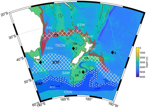
The main near-surface water masses in the north of the region are relatively warm, saline Subtropical Water (STW) and slightly cooler, modified STW known as Tasman Sea Central Water (TSCW), which are separated by the Tasman Front (TF) lying between Australia and northern New Zealand (Heath 1973; Chiswell et al. 2015a). Water found south of STW/TSCW is colder, fresher Subantarctic Water (SAW), and the front separating STW/TSCW from SAW is the Subtropical Front (STF, Heath 1981). In the Tasman Sea, density gradients tend to be weak and geographically mobile, so that it is difficult to define the location of the STF (e.g. Hamilton 2006). East of New Zealand, the STF is topographically locked to the Chatham Rise (Chiswell 2001; Sutton 2001), but then east of the rise it turns to the south (Fernandez et al. 2014). Water found south of SAW is Circumpolar Surface Water (CSW), and the front separating SAW from CSW is the Subantarctic Front (SAF) which is the northern front of the Antarctic Circumpolar Current (ACC, Sokolov and Rintoul 2009).

The STW/TSCW and SAW water masses are considered to be different biomes reflecting the different roles nutrients, light, and mixing play in controlling production within a water mass. STW/TSCW is generally characterised by autumn and spring blooms in SSC, with the timing of the blooms dependent on latitude, whereas SAW is characterised by summer blooms in SSC (Longhurst et al. 1995; Chiswell et al. 2013).

There have been 3 recognised MHWs in the New Zealand region during the last decade. These were in the summers of 2015/16 (Oliver et al. 2018), 2017/19 (Salinger et al. 2019), and most recently in 2018/19 (this article). Despite the considerable interest MHWs have generated globally, there is no universally accepted definition of a MHW, with various definitions requiring SST to be sustained at some threshold temperature above climatology for some critical number of days (e.g. Hobday et al. 2018). Since MHW statistics are not the focus of this article, we do not require precise definitions of when they start or end, but simply identify them as occurring when SST anomalies exceed 3 standard deviations from climatology.

Data

Sea surface temperature

The NOAA 1/4° daily Optimum Interpolation Sea Surface Temperature (OISST) is an objectively-analysed product provided by NOAA. This analysis is constructed by combining observations from different platforms (satellites, ships, buoys) on a regular global grid (NOAA OI SST V2 High Resolution Dataset, Reynolds et al. 2007; Banzon et al. 2016). Here, to ensure consistency through the time series, we use the Advanced Very-High-Resolution Radiometer (AVHRR) only product (https://www.ncdc.noaa.gov/oisst).

Wind stress

The National Centers for Environmental Prediction (NCEP) and the National Center for Atmospheric Research (NCAR), USA, provide reanalysis products from 1948 to the present using assimilation of data. Daily values of wind stress were downloaded from http://www.esrl.noaa.gov/psd/data/gridded/data.ncep.reanalysis.surfaceflux.html.

Sea surface chlorophyll

The Moderate Resolution Imaging Spectroradiometer (MODIS) flying on the Aqua satellite has provided ocean colour measurements of SSC since 2002. Mapped 8-d 9-km composite data were downloaded from NASA’s Ocean Color website (https://oceancolor.gsfc.nasa.gov/).

Net primary production

There are various NPP products available. We use the Vertically Generalized Production Model (VGPM, Behrenfeld and Falkowski 1997b). The VGPM algorithm is based on SSC, SST, euphotic depth, and day length (Behrenfeld and Falkowski 1997a). We should note, however, that the VGPM algorithm has not been tuned or validated for local conditions, and we have little information on how well VGPM represents NPP in the New Zealand region. VGPM data were downloaded from the Ocean Productivity web page https://www.science.oregonstate.edu/ocean.productivity/ for the MODIS time period (from 2002 on).

Vertical Profiles

Argo floats (Gould and Turton 2006) are free-drifting floats that return temperature and salinity water column profiles about every 10 d. Most floats are set to have a nominal ‘parking depth’ of 1000 m and a profiling depth of 2000 m. These parking and profiling depths mean that Argo floats rarely enter regions where the water depth is less than 1000 m. During their time at the surface, Argo floats transmit their latitude and longitude and profile data via satellite. Quality-controlled Argo data are available from Argo’s two Global Data Assembly Centres (GDACs) in Brest, France and Monterey, California. Argo float deployments began in 2000, but the targeted density of 3000 floats globally was not achieved until 2006.

Methods

Satellite estimates of SST extend as far back as 1979. SSC and VGPM extend back as far as the start of the Sea-Viewing Wide Field-of-View Sensor (SeaWIFS) mission in 1997, which was then replaced by the MODIS series of instruments in 2002. However, there is a mismatch between SeaWIFS and MODIS estimates of SSC (Zibordi et al. 2006), so this work is limited to the start of MODIS in 2002 in order to avoid any false inferences in trend caused by this mismatch.

The SST, wind stress, SSC, and NPP products were subsampled on to a 2° grid for analysis. The 8-d records (SSC and NPP) were interpolated to daily values. Annual cycles were then removed from these time series, they were then smoothed with a 15-d running mean window and subsampled at monthly intervals before computing the mean and trends.

A time series of MLD was computed for each 2° grid location using all Argo profiles taken within 500 km of that grid location. MLD was computed as the depth where the local density exceeds the surface density by 0.125 kg m⁻³ – this is a commonly used definition of MLD (e.g. Kara et al. 2000). The winter maximum MLD for each year was taken to be the maximum MLD in the respective calendar year.

Linear trends in the satellite products and winter maximum MLD were computed using standard linear least-squares regression analyses. The significance of the slope was calculated following Santer et al. (2000) as discussed in the Appendix.

Representative sites

Four representative sites (labelled in Figure 1) were chosen to illustrate the data and methods. Figures 2–5 show SST, wind stress magnitude, SSC, NPP, and MLD for each of these representative sites.

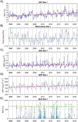
Site 1 is just south-east of Tasmania. At this location SST had a mean value of 14.1°C, with a standard deviation of 1°C (Figure 2). The 2002–18 trend is significant (t-test > 0.95) with a value of ∼0.7°C decade⁻¹. The trend in wind stress is not significantly different from zero. Both SSC and NPP show considerable interannual variability, but show significant positive trends over the 2002–18 period, with values of 0.04 mg m⁻³decade⁻¹, and 67 mg C m⁻² d⁻¹ decade⁻¹, respectively. This site had more Argo profiles than most, but the figure illustrates that even so, there were some years where few or no floats passed within 500 km of the location (e.g. 2015). For the data shown, the MLD_max trend has a value of −14 m decade⁻¹, but is not significant.

Figure 2. Time series of observed quantities at Site 1 (shown in Figure 1) with annual cycles removed. A, Sea surface temperature (SST); B, Wind stress magnitude; C, Sea surface chlorophyll (SSC); D, Net primary production (NPP); E, Mixed layer depth (MLD) derived from Argo profiles taken within 500 km of the site. Red circles indicate the deepest MLD in each year. Also shown are linear trends fit to the data (red dashed line if significant, green dashed line if not significant).

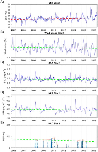
Site 2 is in eastern Tasman Sea near the Challenger Plateau. SST from this site has a mean value of 15.9°C and standard deviation of 0.8°C (Figure 3). The 2017/18 MHW can be seen where SST reached 20°C (more than 4 standard deviations from the mean) in late 2017. SST has a significant trend of 0.29°C decade⁻¹. However, the trends in wind stress, SSC, and NPP are not significant. The Challenger Plateau is shallower than 1000 m deep, and the MLD is very poorly sampled for this site largely because the Argo program targets deeper water. The calculated negative trend in MLD_max is not significant.

Figure 3. Time series of observed quantities at Site 2 (shown in Figure 1) with annual cycles removed. A, Sea surface temperature (SST); B, Wind stress magnitude; C, Sea surface chlorophyll (SSC); D, Net primary production (NPP); E, Mixed layer depth (MLD) derived from Argo profiles taken within 500 km of the site. Red circles indicate the deepest MLD in each year. Also shown are linear trends fit to the data (red dashed line if significant, green dashed line if not significant).

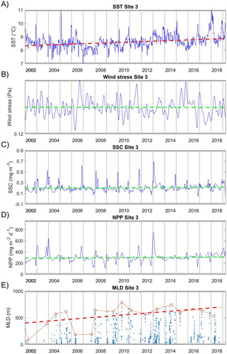
Site 3 is in SAW over the Campbell Plateau east of the South Island. SST from this site has a mean value of 8.6°C and standard deviation of 0.5°C (Figure 4). While SST was warm at the end of 2017, it was only 2 standard deviations above the mean, indicating the 2017/18 MHW had less impact in this region than at Sites 1 and 2. SST showed a significant trend of 0.3°C decade⁻¹. Wind stress, SSC, and NPP show no significant trend. Few Argo floats passed near this site before 2004 and in 2006 and 2007, however the trend in MLD_max was returned as significant with a value of 176 m decade⁻¹.

Figure 4. Time series of observed quantities at Site 3 (shown in Figure 1) with annual cycles removed. A, Sea surface temperature (SST); B, Wind stress magnitude; C, Sea surface chlorophyll (SSC); D, Net primary production (NPP); E, Mixed layer depth (MLD) derived from Argo profiles taken within 500 km of the site. Red circles indicate the deepest MLD in each year. Also shown are linear trends fit to the data (red dashed line if significant, green dashed line if not significant).

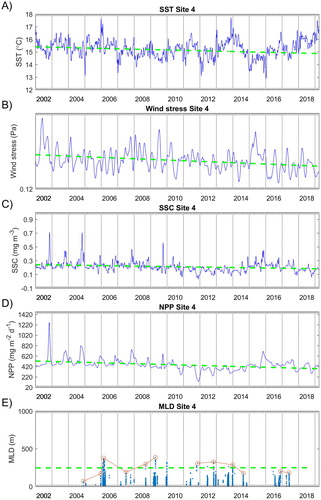
Site 4 is east of the North Island in STW. SST had a mean value of 15.3°C with a standard deviation of 0.7°C (Figure 5). Whilst SST, SSC and NPP all showed negative trends, they were not significantly different from zero. Relatively few Argo floats passed near this site in winter, so that winter MLD was poorly sampled. The calculated trend in MLD_max at this site was not significant.

Figure 5. Time series of observed quantities at Site 4 (shown in Figure 1) with annual cycles removed. A, Sea surface temperature (SST); B, Wind stress magnitude; C, Sea surface chlorophyll (SSC); D, Net primary production (NPP); E, Mixed layer depth (MLD) derived from Argo profiles taken within 500 km of the site. Red circles indicate the deepest MLD in each year. Also shown are linear trends fit to the data (red dashed line if significant, green dashed line if not significant).

These figures illustrate that while one can make confident estimates of changes in SST, and to a lesser extent, SSC, it is a major challenge to determine confident estimates of changes in MLD_max. For example, at Site 3, the trend in MLD_max was returned as significant largely because of the low MLD seen in 2002, 2006 and 2007, even though it we can be reasonably confident that these low values do not represent winter mixing. Rather than make subjective decisions as to whether MLD from individual profiles represents winter mixing, we retained all profiles in our analyses.

Results

Mean fields

Figure 6 shows the mean SST, wind stress, SSC, NPP, and MLD for the period 2002–18. These fields illustrate the well-known physical and biogeochemical processes in the region, (e.g. Murphy et al. 2001; Chiswell et al. 2013; Chiswell et al. 2015a), with warmer STW and low wind stress to the north, and cooler SAW/CSW and high wind stress due to westerly winds in the south. Mean MLD is less than 50 m to the north, with deepest mean MLD (>200 m) coincident with the region of strongest mean wind stress and weaker stratification underlaying CSW.

Figure 6. Mean fields computed from 2002 to 2018. A, Sea surface temperature (SST); B, Wind stress magnitude; C, Sea surface chlorophyll (SSC); D, Net primary production estimated from the Vertically Generalized Production Model (VGPM); E, Mixed layer depth (MLD). Four representative locations are labelled 1 to 4. The dashed lines indicate maxima in SSC along the Subtropical Front.

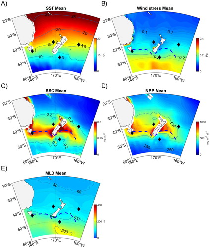
Outside of the coastal regions, highest SSC lies along the STF in a band extending from Tasmania to New Zealand, and then along the Chatham Rise east of New Zealand (as indicated by the dashed line in the figure). Mean NPP largely follows SSC, but is skewed towards warmer waters, reflecting the influence of SST and day length in the VGPM algorithm. NPP reaches 700 mg m² d⁻¹ along the band of highest SSC.

Inter-annual variability

Hovmöller diagrams are often a useful tool to visualise relationships between variables, and so are used here to illustrate the interannual variability. Anomalies in SST and SSC were computed from the 15-d smoothed data by removing the respective mean and annual cycle (but not trend) at each location. These data were then divided into two regions. The first region is denoted ‘Tasman Sea’ and includes all data between 155°E and 170°E chosen to avoid most of the East Australian Current. The second region is denoted ‘East of New Zealand’ and includes all data between 180°E and 160°W. Hovmöller diagrams of the zonally-averaged anomalies for each region are shown in Figure 7.

Figure 7. A,B, Hovmöller diagram of sea surface temperature (SST) and sea surface chlorophyll (SSC) anomalies zonally averaged across the Tasman Sea between 150°E and 175°E; C,D, Hovmöller diagram of SST and SSC anomalies zonally averaged from 180° to 160°W. Anomalies are computed by removing the mean and annual cycle (but not linear trend) from the respective quantities. Contours where the anomaly exceeds ± 3 s.d. are shown for each variable. SST anomaly contours are shown on the SSC plots and vice versa.

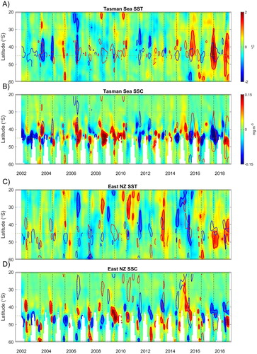
In the Tasman Sea (Figure 7A,B), cool anomalies dominate the early part of the record and warm anomalies dominate the latter part of the record, reflecting the long-term trend in SST. In addition, there is a clear change in character near 45°S – anomalies rarely exceed 3 s.d. south of this latitude. North of 45°S, the most obvious features are the MHWs of 2015/16, 2017/18 and 2018/19. There was also a warm event in 2005/06 that has not been regarded as a MHW, and cool events in 2004, 2006/07, and 2012. There are no winter SSC data south of 45°S because winter day lengths at high latitudes preclude ocean colour measurements. North of 45°S, there is a tendency for positive SST anomalies to coincide with negative SSC anomalies, and vice versa. For example, the MHWs of 2015/16 and 2017/18 coincided with negative SSC anomalies, the cool SST event in 2006/7 coincided with positive SSC anomaly, and the positive SSC anomaly of 2008/09 coincided with cooler than usual SST. However, the relationships are not perfect, for example, the 2018/19 MHW appears to be associated with positive SSC anomaly.

East of New Zealand (Figure 7C,D) shows different behaviour, and there is little correlation between SST anomalies east of New Zealand and those in the Tasman Sea. For example, 2015 and 2016 were generally warmer than normal in the Tasman Sea, but cooler than normal east of New Zealand. Conversely, 2003 and 2004 were cooler in the Tasman Sea but warmer east of New Zealand, although 2007 was cooler in both domains. East of New Zealand, there appears to be some coincidence between SST and SSC anomalies north of 45°S. For example, most of the positive anomalies in SSC north of 45°S were coincident with negative SST anomalies. There is a clear change in character at 45°S, with many cases where positive and negative anomalies occur either side of this latitude at the same time.

2002–18 trends

The 2002–18 trends for all variables are shown in Figure 8. Regions where the trend is not locally considered significant are overlaid with cross-hatching. Dashed lines along the peaks in mean SSC seen in Figure 6 are shown for comparison between fields (these lines approximately overlay the mean position of the STF).

Figure 8. Trends computed from over 2002 to 2018. A, Sea surface temperature (SST); B, Wind stress magnitude; C, Sea surface chlorophyll (SSC); D, Net primary production (NPP) estimated from the Vertically Generalized Production Model; E, Maximum winter mixed layer depth (MLD_max). Blue dashed lines drawn through the maxima in mean SSC (Figure 6) and red dashed lines drawn through the maxima in SSC trend are included to aid comparison between fields. Black diamonds show the representative sites shown in Figure 1.

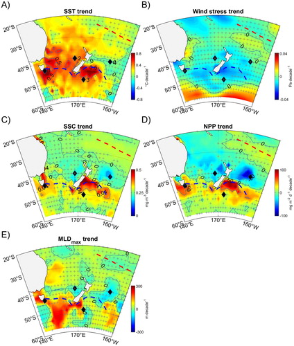
The most robust trend is for SST, where most of the region showed warming, although not all is significant. Highest warming occurred off the east coast of Australia, reaching 0.7°C decade⁻¹, with warming over the entire Tasman Sea, and over the Chatham Rise. However, north of, and east of the Chatham Rise, the trend indicates cooling up to 0.1°C decade⁻¹, although this is not significant.

The trend in wind stress is not significant over much of domain, although there was significant strengthening of the westerlies near 55°S, and weakening over much of the STF. The strongest warming in SST coincided with generally weakening wind stress – except over the EAC.

The trend in SSC shows significant positive values in two regions. The largest trends, reaching 0.04 mg m⁻³decade⁻¹ are found along the band of highest mean SSC coincident with the STF (compare with Figure 6). There is another region of significant positive trend in the north-east of the domain as shown by the red dashed lines in Figure 8. This band of positive trend is coincident with the region of high variability in sea surface height associated with the South Pacific Subtropical Counter Current (SP STCC, Qiu and Chen 2004; Travis and Qiu 2017). We refer to this band as the subtropical band. Over much of the Tasman Sea, east of New Zealand, and over the SAF, the SSC trend is negative and not significant.

The trend in NPP largely mimics that in SSC, with positive trends along the STF and subtropical band, whereas most of the Tasman Sea and the region east of New Zealand shows significant negative trend. The trend in NPP reaches 50 mg C m⁻² d⁻¹ decade⁻¹ in SAW over the Chatham Rise.

The trend in MLD_max, although not significant almost everywhere shows a spatial pattern which has some characteristics of the pattern of SSC trend. There is a region of deepening MLD_max in the south Tasman Sea over the STF, approximately coincident with bands in SSC and NPP trends. Shallowing trends in MLD_max in the eastern Tasman Sea and east of New Zealand coincide with regions of decreasing SSC and NPP. In contrast, however, deepening trends in MLD_max in the northern Tasman Sea also coincide with weak or decreasing SSC and NPP.

We return to a more complete discussion of these trends later, but for now we note that while SST warmed nearly everywhere, SSC and NPP showed increases over the STF and subtropical band, but decreases over most of the Tasman Sea and east of New Zealand. While there may a connection between wind stress and SST trends, there is no obvious connection between wind stress and SSC or NPP trends.

Correlation between SSC and SST variability

For each location in the domain, we computed the linear least-squares fit between SST and SSC detrended anomalies, i.e. the time series shown in Figures 2–5 (panels A and C), but with trends removed to ensure the regression is not influenced by correlation between the long-term changes. The slope of the regression largely mimics the SSC trend with positive values south of the STF and negative values north of the front (Figure 9). This suggests that at monthly timescales, increased SSC is associated with warm anomalies south of the STF, and vice-versa north of the STF.

Figure 9. A, Slope of the linear regression between sea surface chlorophyll (SSC) and sea surface temperature (SST). This slope was computed from the detrended 30-d subsampled time series (e.g. those seen in Figure 2); B, The slope of the linear regression between mean October to December SSC and the preceding mid-winter minimum SST. Locations where the slope was considered not significantly different from zero are shown with cross-hatching. The dashed lines are as shown in Figure 8.

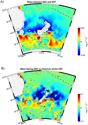
This simple analysis does not address any mechanisms linking primary production and warmer oceans, and in particular, does not address the paradigm that primary production in the spring is limited by the previous winter deep mixing. To address this paradigm, we assume the coolest winter SST at each location is a proxy for the depth of deepest winter mixing, and that the mean SSC from October to December is a proxy for total spring production. When plotted spatially, the slope of mean spring SSC vs preceding winter minimum SST (Figure 9B), much like the SST trend (Figure 8), shows generally positive values along and south of the STF, negative values in the eastern Tasman Sea and east of New Zealand, and weakly positive values in the western Tasman Sea.

Discussion

The most robust of our estimates is the SST trend, both because SST can be measured with high accuracy (AVHRR-based estimates of SST are more accurate than MODIS estimates of SSC), and because there is a relatively strong signal. We should re-emphasise, however, that trends are susceptible to the length of the time series they are calculated from, and that especially in the eastern Tasman Sea, our trends are influenced by the 3 recent MHWs. Consequently our 2002–18 trends show differences from the 1981–2017 trends of Sutton and Bowen (2019), who found highest warming off the east coast of Australia (in agreement with us), but east of New Zealand they found cooling south of the Chatham Rise and strong warming north of the rise, whereas we found almost the opposite – warming south of the rise and no warming north of the rise.

Our next most robust estimate is the SSC trend. This suggests that we can have confidence in the observation that SSC increased along the STF and in the subtropical band (the red dashed lines in Figure 8), but decreased in the eastern Tasman Sea and to the east of New Zealand. Following this in robustness is the NPP trend, reflecting the VGPM algorithm dependence on SST and SSC, although as noted before, we have little evaluation of VGPM as a measure of NPP in the New Zealand region.

Our least robust calculation is the trend in MLD_max. At almost every 2° grid point, the calculated trend is not significant, and even where it is calculated as significant, we cannot be sure that this is not due to fortuitous temporal sampling of the Argo floats. Yet when plotted spatially, the MLD_max trend broadly mimics the SSC trend showing highest trend over the STF. Given we have an a priori expectation that production should follow MLD_max, this suggests that on average, the low spatial and temporal Argo sampling rates may lead to high noise rather than bias in computing trends.

Overall, we can be fairly certain that despite long-term warming over almost the entire region, SSC and NPP increased along the STF and in the subtropical band (Figure 8). We have confidence that SSC anomalies are negatively correlated with SST anomalies north of the STF and vice-versa over the STF (Figure 7). We have some confidence that spring SSC is negatively correlated with the previous winter minimum SST north of the STF and vice-versa south of the front (Figure 9). With the least amount of confidence, we have a suggestion that trends in surface biomass correlate positively with trends in deep winter mixing almost everywhere (Figure 8).

Taken together, these observations suggest that the paradigm that any future warming will lead to shallower winter mixing and less primary production can hold only in the Tasman Sea north of the STF, and east of New Zealand. Elsewhere, especially over the STF, either the opposite holds or there is no significant relationship.

It is interesting to compare our observed trends with predicted changes under the business-as-usual scenario, RCP 8.5, from the Coupled Model Intercomparison Project 5 (CMIP5) models (Bopp et al. 2013) and the Community Earth System Model (CESM, Krumhardt et al. 2017). Bopp et al. (2013), for 2090–99 relative to 1990–99, predict NPP will show small positive trends over the STF, and negative changes north of New Zealand. For 2080 compared to 1920, Krumhardt et al. (2017) predict NPP patterns much more similar to those presented here with strong increases over STF and decreases in the Tasman Sea. Neither study shows increases in SP STCC region.

The STF coincides with the transition from the South Pacific Subtropical gyre (SPSG) to Subantarctic (SANT) biomes as listed by Longhurst et al. (1995). SPSG is dominated by winter and spring blooms and low summer surface production (Chiswell et al. 2015b). In these waters, surface spring blooms terminate with depleted nutrients in early summer (e.g. Boyd et al. 2012). Although it is not clear whether macronutrients (nitrate, phosphate) or micronutrients (iron) limit total production, it seems feasible that the nutrient supply controls total production. In contrast, SANT is dominated by summer production (Chiswell et al. 2015b), because it is only in summer that there is sufficient light for production. In these ‘High-nitrate low-chlorophyll’ waters, the macro-nutrients are not limiting, instead the production is often iron-limited (Venables and Moore 2010). Under these circumstances it is possible that longer summer (warmer SST) conditions lead to a longer growing season, but there may be other reasons for a positive trend in NPP, such as increased terrigenous iron into these iron-limited waters. Thus, the change in the relationships between warming and production at the STF is likely indicative of different biological processes in the two water masses.

Even though we conclude that the warming paradigm can hold only regionally in STW, evidence that the MLD_max trend generally matches the SSC trend over most of the region (Figure 8C), suggests not only that long-term trends in production might be controlled by deep winter mixing everywhere, but that in SAW especially, there are areas where deep winter mixing increased even where surface waters warmed.

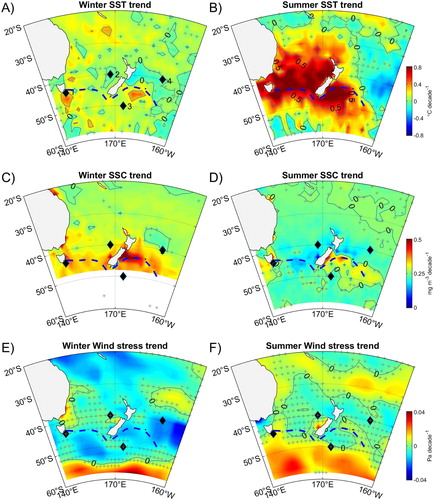
It is not obvious how surface waters can warm while the MLD_max deepens. When trends are computed separately over winter (June-August) and summer (December-February), winter SST trends tend to be near zero or only weakly positive compared to strong positive summer trends (Figure 10A,B). It seems that the long-term trend towards rising SST is due to warmer summers, with a contribution from summer MHWs, rather than year-round warming. Even so, winter SST does not show decreases that would be expected with deepening winter MLD. It may be that any deepening of the mixed layer is due to a northward shift in the Antarctic Circumpolar Current (i.e. a northwards shift of the band of deep mixed layer seen near 50°S in Figure 6).

Figure 10. Trends in quantities computed from 2002 to 2018 for winter (June-August) and summer (December-February). A, Winter sea surface temperature (SST) trend; B, Summer SST trend; C, Winter sea surface chlorophyll (SSC) trend (winter satellite coverage is insufficient to compute trend south of ∼48°S); D, Summer SSC trend; E, Winter wind stress magnitude trend; F, Summer wind stress magnitude trend.

We should note that SSC is at best an imprecise measure of near-surface primary biomass, and is not necessarily indicative of depth-integrated production or of carbon exported to higher trophic levels (Behrenfeld et al. 2016). Given that VGPM has not been verified for the New Zealand region, and given the question of how well regional trends in mixed layer depth can be estimated from Argo data, studies such as this give insight into, rather than quantify the oceanic processes determining primary production. A better understanding of climate changes in the ocean needs to be derived from longer time periods and well-calibrated and evaluated models.

Finally, we comment on the impact of MHWs on production. MHWs contribute to some of the variability leading to the correlation shown in Figure 9, but the Hovmöller diagrams suggest that not all MHWs impact production in the same way. For example, in the Tasman Sea, the responses to the MHWs of 2015/16 and 2016/17 were decreases in SSC, whereas the response to the 2018/19 MHW was an increase in SSC. Even where MHWs lead to a decrease in near surface biomass, the mechanisms are unlikely to be related to the previous winter’s deep mixing since the MHWs are shallow, and likely due to local anomalously low wind stress (Salinger et al. 2019). Instead, it is likely that MHWs strengthen the summer thermocline thus shutting of any summer time resupply of nutrients from below and so further shut down summer time near-surface production.

Conclusions

The main objective of this research was to investigate whether the paradigm that warming oceans lead to deceased net primary production holds in the New Zealand region by considering previous variability and trends in warming and production.

We conclude that this paradigm is unlikely to hold over the STF and it may not hold in the subtropical waters of the SP STCC, or in SAW. Over the Tasman Sea, and much of the STW surrounding New Zealand, we expect this paradigm will hold.

Acknowledgements

We thank NOAA, NASA and NCEP for making the various SST, SSC, VGPM and reanalysis products freely available. NOAA High Resolution SST data were produced by NOAA/NCEI (https://www. ncdc.noaa.gov/oisst) and provided from the NOAA/OAR/ESRL PSD, Boulder, Colorado, USA, website (http://www.esrl.noaa.gov/psd/). Argo data were collected and made freely available by the International Argo Program and the national programmes that contribute to it (http://www.argo.ucsd.edu, http://argo.jcommops.org). The Argo Program is part of the Global Ocean Observing System.

Disclosure statement

No potential conflict of interest was reported by the authors.

Additional information

Funding

This work was supported by the New Zealand Ministry of Business, Innovation and Employment through grants to NIWA’s climate change and coastal ocean programmes.

Appendix. Significance of least-squares regression

Least-squares regression produces a linear estimate$\hat{Y}=ax+b,$where a and b are the slope and intercept of the regression. The significance of the slope was calculated following Santer et al. (2000). First the standard error of the slope was calculated as$s_a=\frac{s_e}{{\left[\mathrm{\Sigma }{(x-\overline{x})}^2\right]}^{1/2}}.$where $s_e^2$ is the variance of the residuals about the regression. We then compute the slope divided by its standard error$t_a=a/s_a.$Whether the slope is significantly different from zero or not at a defined significance level, α, can be determined by assuming t_a is distributed as Student’s t distribution with n degrees of freedom. That is, the null hypothesis is that the regression has no slope. If t_a exceeds the significance level, then one can reject the null hypothesis.

The significance of each trend was tested using the Matlab routine tcdf.m which returns the Student’s t cumulative distribution function estimate given the number of degrees of freedom. A value greater than 0.95 was considered significant (p < 0.05).

For the monthly subsampled satellite products, the sampling period is about one Eulerian timescale (Chiswell and Rickard 2008; Chiswell 2013), so we assumed each estimate was independent. Trends for the deepest winter MLD were computed from yearly values which we also assumed are independent. Thus, for both satellite and Argo products, the number of degrees of freedom was the record length minus 2.

References

- Banzon V, Smith TM, Chin TM, Liu C, Hankins W. 2016. A long-term record of blended satellite and in situ sea-surface temperature for climate monitoring, modeling and environmental studies. Earth System Science Data. 8(1):165–176. DOI:10.5194/essd-8-165-2016.
- Behrenfeld M, Falkowski PG. 1997a. A consumer’s guide to phytoplankton primary productivity models. Limnology and Oceanography. 42(7):1479–1491. DOI:10.4319/lo.1997.42.7.1479.
- Behrenfeld MJ, Falkowski PG. 1997b. Photosynthetic rates derived from satellite-based chlorophyll concentration. Limnology and Oceanography. 42(1):1–20. DOI:10.4319/lo.1997.42.1.0001.
- Behrenfeld MJ, O’Malley RT, Boss ES, Westberry TK, Graff JR, Halsey KH, Milligan AJ, Siegel DA, Brown MB. 2016. Revaluating ocean warming impacts on global phytoplankton. Nature Climate Change. 6(3):323–330. DOI:10.1038/nclimate2838.
- Bopp L, Resplandy L, Orr JC, Doney SC, Dunne JP, Gehlen M, Halloran P, Heinze C, Ilyina T, Séférian R, et al. 2013. Multiple stressors of ocean ecosystems in the 21st century: projections with CMIP5 models. Biogeosciences. 10(10):6225–6245. DOI:10.5194/bg-10-6225-2013.
- Boyd PW, Strzepek R, Chiswell S, Chang H, DeBruyn JM, Ellwood M, Kenan S, King A, Maas E, Nodder S, et al. 2012. Microbial control of diatom bloom dynamics in the open ocean. Geophysical Research Letters. 39(18):L18601. DOI:10.1029/2012GL053448.
- Chiswell SM. 2001. Eddy energetics in the subtropical front over the Chatham Rise. New Zealand Journal of Marine and Freshwater Research. 35:1–15. DOI:10.1080/00288330.2001.9516975.
- Chiswell SM. 2013. Lagrangian time scales and eddy diffusivity at 1000 m compared to the surface in the south Pacific and Indian oceans. Journal of Physical Oceanography. 43(12):2718–2732. DOI:10.1175/JPO-D-13-044.1.
- Chiswell SM, Bostock HC, Sutton PJH, Williams MJM. 2015a. Physical oceanography of the deep seas around New Zealand: a review. New Zealand Journal of Marine and Freshwater Research. 49(2):286–317. DOI:10.1080/00288330.2014.992918.
- Chiswell SM, Bradford-Grieve J, Hadfield MG, Kennan SC. 2013. Climatology of surface chlorophylla, autumn-winter and spring blooms in the southwest Pacific Ocean. Journal of Geophysical Research: Oceans. 118(2):1003–1018. DOI:10.1002/jgrc.20088.
- Chiswell SM, Calil PHR, Boyd PW. 2015b. Spring blooms and annual cycles of phytoplankton: a unified perspective. Journal of Plankton Research. 37(3):500–508. DOI:10.1093/plankt/fbv021.
- Chiswell SM, Rickard GJ. 2008. Eulerian and Lagrangian statistics in the Bluelink numerical model and AVISO altimetry: validation of model eddy kinetics. Journal of Geophysical Research. 113(C10). DOI:10.1029/2007JC004673.
- Daly EA, Brodeur RD, Auth TD. 2017. Anomalous ocean conditions in 2015: impacts on spring Chinook salmon and their prey field. Marine Ecology Progress Series. 566:169–182. DOI:10.3354/meps12021.
- Eder J. 2018 Feb 2. Hotter-than-normal water kills off salmon in the Sounds. The Marlborough Express.
- Fernandez D, Bowen M, Carter L. 2014. Intensification and variability of the confluence of subtropical and subantarctic boundary currents east of New Zealand. Journal of Geophysical Research: Oceans. 119(2):1146–1160. DOI:10.1002/2013JC009153.
- Gould WJ, Turton J. 2006. Argo – sounding the oceans. Weather. 61(1):17–21. DOI:10.1256/wea.56.05.
- Hamilton LJ. 2006. Structure of the subtropical front in the Tasman Sea. Deep Sea Research Part I: Oceanographic Research Papers. 53(12):1989–2009. DOI:10.1016/j.dsr.2006.08.013.
- Hannan P. 2019 Mar 3. ‘ Not very happy’: Tasman Sea warmth puts the heat on key fisheries. The Sydney Morning Herald.
- Heath RA. 1973. Present knowledge of the oceanic circulation and hydrology around New Zealand-1971. Tuatara. 20(3):125–140.
- Heath RA. 1981. Oceanic fronts around southern New Zealand. Deep Sea Research Part A. Oceanographic Research Papers. 28(6):547–560. DOI:10.1016/0198-0149(81)90116-3.
- Hobday A, Oliver E, Sen Gupta A, Benthuysen J, Burrows M, Donat M, Holbrook N, Moore P, Thomsen M, Smale D, et al. 2018. Categorizing and naming marine heatwaves. Oceanography. 31(2). DOI:10.5670/oceanog.2018.205.
- Hulburt P. 2018 Jun 3. Salmon industry in short supply turns to Atlantic seas for help. The Marlborough Express.
- Kara AB, Rochford PA, Hurlburt HE. 2000. An optimal definition for ocean mixed layer depth. Journal of Geophysical Research: Oceans. 105(C7):16803–16821. DOI:10.1029/2000JC900072.
- Krumhardt KM, Lovenduski NS, Long MC, Lindsay K. 2017. Avoidable impacts of ocean warming on marine primary production: insights from the CESM ensembles. Global Biogeochemical Cycles. 31(1):114–133. DOI:10.1002/2016GB005528.
- Law CS, Rickard GJ, Mikaloff-Fletcher SE, Pinkerton MH, Behrens E, Chiswell SM, Currie K. 2017. Climate change projections for the surface ocean around New Zealand. New Zealand Journal of Marine and Freshwater Research. 1–27. DOI:10.1080/00288330.2017.1390772.
- Longhurst A, Sathyendranath S, Platt T, Caverhill C. 1995. An estimate of global primary production in the ocean from satellite radiometer data. Journal of Plankton Research. 17(6):1245–1271. DOI:10.1093/plankt/17.6.1245.
- Lozier MS, Dave AC, Palter JB, Gerber LM, Barber RT. 2011. On the relationship between stratification and primary productivity in the north Atlantic. Geophysical Research Letters. 38(18):1–6. DOI:10.1029/2011GL049414.
- Murphy RJ, Pinkerton MH, Richardson KM, Bradford-Grieve JM, Boyd PW. 2001. Phytoplankton distributions around New Zealand derived from SeaWiFS remotely-sensed ocean colour data. New Zealand Journal of Marine and Freshwater Research. 35(2):343–362. DOI:10.1080/00288330.2001.9517005.
- Oliver ECJ, Lago V, Hobday AJ, Holbrook NJ, Ling SD, Mundy CN. 2018. Marine heatwaves off eastern Tasmania: trends, interannual variability, and predictability. Progress in Oceanography. 161:116–130. DOI:10.1016/j.pocean.2018.02.007.
- Qiu B, Chen S. 2004. Seasonal modulations in the eddy field of the south Pacific Ocean. Journal of Physical Oceanography. 34(7):1515–1527. DOI:10.1175/1520-0485(2004)034<1515:SMITEF>2.0.CO;2.
- Reynolds RW, Smith TM, Liu C, Chelton DB, Casey KS, Schlax MG. 2007. Daily high-resolution-blended analyses for sea surface temperature. Journal of Climate. 20(22):5473–5496. DOI:10.1175/2007JCLI1824.1.
- Rickard GJ, Behrens E, Chiswell SM. 2016. CMIP5 earth system models with biogeochemistry: an assessment for the southwest Pacific Ocean. Journal of Geophysical Research: Oceans. 121(10):7857–7879. DOI:10.1002/2016JC011736.
- Salinger MJ, Renwick J, Behrens E, Mullan AB, Diamond HJ, Sirguey P, Smith RO, Trought MCT, Alexander V L, Cullen NJ, et al. 2019. The unprecedented coupled ocean-atmosphere summer heatwave in the New Zealand region 2017/18: drivers, mechanisms and impacts. Environmental Research Letters. 14(4):044023. DOI:10.1088/1748-9326/ab012a.
- Santer BD, Wigley TML, Boyle JS, Gaffen DJ, Hnilo JJ, Nychka D, Parker DE, Taylor KE. 2000. Statistical significance of trends and trend differences in layer-average atmospheric temperature time series. Journal of Geophysical Research: Atmospheres. 105(D6):7337–7356. DOI:10.1029/1999JD901105.
- Shears NT, Bowen MM. 2017. Half a century of coastal temperature records reveal complex warming trends in western boundary currents. Science Reports. 7(1):14527. DOI:10.1038/s41598-017-14944-2.
- Sokolov S, Rintoul SR. 2009. Circumpolar structure and distribution of the Antarctic Circumpolar Current fronts: 1. Mean circumpolar paths. Journal of Geophysical Research. 114(C11018). DOI:10.1029/2008jc005108.
- Somavilla R, Gonzalez-Pola C, Fernandez-Diaz J. 2017. The warmer the ocean surface, the shallower the mixed layer. How much of this is true? Journal of Geophysical Research-Oceans. 122(9):7698–7716. DOI:10.1002/2017JC013125.
- Sutton P. 2001. Detailed structure of the subtropical front over Chatham Rise, east of New Zealand. Journal of Geophysical Research. 106(C12):31045–31056. DOI:10.1029/2000JC000562.
- Sutton PJH, Bowen M. 2019. Ocean temperature change around New Zealand over the last 36 years. New Zealand Journal of Marine and Freshwater Research 53(3):305–326. doi: 10.1080/00288330.2018.1562945
- Travis S, Qiu B. 2017. Decadal variability in the South Pacific Subtropical Countercurrent and regional mesoscale eddy activity. Journal of Physical Oceanography. 47(3):499–512. DOI:10.1175/JPO-D-16-0217.1.
- Venables H, Moore CM. 2010. Phytoplankton and light limitation in the Southern Ocean: learning from high-nutrient, high-chlorophyll areas. Journal of Geophysical Research. 115(C2). DOI:10.1029/2009JC005361.
- Zibordi G, Mélin F, Berthon J-F. 2006. Comparison of SeaWiFS, MODIS and MERIS radiometric products at a coastal site. Geophysical Research Letters. 33(6). DOI:10.1029/2006GL025778.