The impact of high rainfall events on the submesoscale salinity field in a coastal sea: Greater Cook Strait, New Zealand

ABSTRACT

River inflow into the coastal oceanic environment can result in low salinity submesoscale features (LSMFs). The enhanced water column stability sustained within these coherent structures affects local biological productivity. With-event and seasonal variability of LSMFs were investigated in a coastal sea -- Greater Cook Strait -- that is characterised by strong tidal and wind forcing as well as being forced at the land-sea boundary by several major rivers. A combination of ocean glider and satellite observations revealed the existence of seasonal variability in temperature, chlorophyll and stratification in LSMFs. High rainfall from ex-cyclone enhanced production of LSMFs in seasons when they would otherwise be less frequent. Stronger stratification was observed at the end of spring, in summer and at the beginning of autumn both in ambient shelf conditions and within LSMFs. Subsurface chlorophyll-a maxima were found associated with summer and spring LSMFs, when temperature had a stronger contribution to vertical stratification. In the available samples, LSMFs were advected seawards when river discharges exceeded 600 m${}^3$ s${}^{-1}$. When river flows were lower than this threshold, other drivers such as wind or currents were required to advect the observed LSMFs offshore.

KEYWORDS:

• River plume
• coastal stratification
• ocean glider
• submesoscale
• region of freshwater influence

1. Introduction

River inputs to coastal seas can influence ocean dynamics well beyond near-field river discharges. Freshwater buoyancy contributions at the surface can maintain strong horizontal and vertical salinity gradients in the far-field continental shelf seas (Simpson and Sharples 2012). Lateral and vertical gradients in upper ocean density, namely fronts and stratification, regulate ocean dynamics. These stratified fronts can set up baroclinic instability while vertical gradients convert potential energy to kinetic energy in the ocean (Fox-Kemper et al. 2008). When combined spatially, these dynamics can result in the conversion of horizontal density gradients to stratification over submesoscale scales, i.e. 1–10 km (Jaeger and Mahadevan 2018). Winds stress and surface buoyancy fluxes can develop into submesoscale instabilities (Gommenginger et al. 2019; Mahadevan 2019) or low salinity submesoscale features (LSMFs, Jhugroo et al. 2020). The result is the river input breaks down into coherent structures sustaining a variety of thermohaline signatures (Figure 1).

Figure 1. Synthesis of A, drivers showing physical processes (wind, storms, rain, rivers) that forms a regional of freshwater influence (RoFI) that then evolves into LSMFs entrained and evolving in the coastal current and B, an elevation view of LSMF details and sampling perspective (MLD mixed layer depth, Chl-a chlorophyll-a, ρ density).

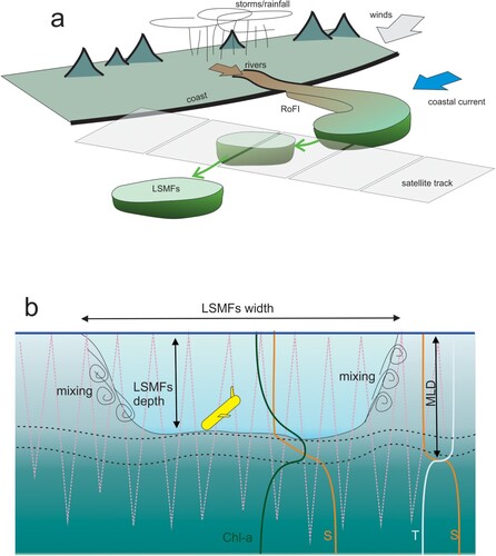
Biological processes can be modulated by ocean state and variability (Simpson and Sharples 2012). The presence of LSMFs promotes stable stratification, shoaling of the mixed layer depth, and inhibits vertical mixing (Figure 1), thus impacting on light and nutrient availability within LSMFs. Lévy et al. (2018) suggest that vertical stratification associated with LSMFs might limit their influence on biological function. This requires assessment of the range of vertical structures possible in LSMFs. In addition, this interplay of vertical stratification, mixing and light with horizontal boundaries in scale influences biological community structure.

Identifying the conditions that lead to the formation of LSMFs requires an understanding of the competition between horizontal and vertical stratification and stability. LSMFs have recently been identified in the Greater Cook Strait region in Aotearoa New Zealand (Jhugroo et al. 2020). Although the system is dominated by strong wind and tidal forcing, weak-to-moderate LSMFs were evident throughout the annual cycle (Figure 2). Offshore advection and lifetime of LSMFs are further modulated by the strength of a coastal barotropic current. LSMFs can be considered as an evolution into the submesoscale of a Region of Freshwater Influence (ROFI), with the latter more closely associated with near-field river source dynamics (Simpson 1997).

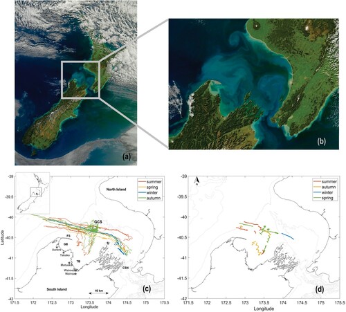
Figure 2. A, True colour image of New Zealand and B, Greater Cook Strait. True colour image obtained by NASA's Aqua MODIS satellite for 29 April 2011; available on NASA's earth observatory. C, Greater Cook Strait showing all glider tracks with a New Zealand map inset and D, glider locations during all sampled LSMFs. Line colour indicates seasonal affiliation of each glider survey and LSMF on C and D, respectively. For glider surveys that spanned over two seasons, the line colour for seasonal affiliation was chosen depending on which season the glider spent most days sampling. GCS: Greater Cook Strait, CSN: Cook Strait Narrows, GB: Golden Bay, TB: Tasman Bay, FS: Farewell Spit, SI: Stephen Island. Grey stars indicate geographical locations of Aorere, Takaka, Motueka, Waimea and Wairoa River gauges.

As LSFMs are primarily a result of salinity anomalies, nearly three quarters of LSMFs (73%) do not exhibit a surface temperature signal (Jhugroo et al. 2020). This means LMSFs are not regularly detectable by satellite observations and so related quantities of phytoplankton biomass and timing of peak biomass can also be underestimated (Lévy et al. 2018). Emerging satellite technologies (e.g. SWOT) are observing higher spatial and temporal submesoscale dynamics. However, subsurface biophysical properties will continue to be difficult to quantify remotely.

Here, we investigate the seasonal variability in the physical and biological characteristics of LSMFs using both in-situ ocean glider data and satellite observations. Ocean gliders, with their ability to collect many hundreds of profiles in a single mission, with multiple sensors, provide a significant increase in data richness with which to examine questions relating to coastal salinity and association biological response. However, with such large, rich datasets come the complex challenge of interpreting the data in the context of motivating questions. A multi-year biophysical dataset was used to examine the following: How do the biophysical characteristics of LSMFs vary seasonally? Is there year-to-year differences in LSMFs productivity for each season? How does the presence of high rainfall weather events influence LSMF occurrence, extent and productivity? Section 2 provides details of the regional setting, while methods and analysis are outlined in Section 3. Seasonal and event variability of LSMFs and associated responses of subsurface chlorophyll-a are examined in Section 4. LSMF dynamics for typical forcing and ex-tropical cyclone events were discussed in Section 5 to provide a perspective of the role salinity-induced submesoscale features in coastal seas.

2. Regional setting: Greater Cook Strait

Greater Cook Strait (Te Moana o Raukawa) is the shelf sea between the North and South Islands of Aotearoa New Zealand (Figure 2). It comprises Golden Bay, Tasman Bay, South Taranaki Bight and the Narrows (Figure 2C). The 135-km-wide western entrance reduces to a 24-km-wide section (The Narrows) in the south east region of Greater Cook Strait. Water depths typically vary from 40 to 150 m, but shoal to less than 40 m in the coastal bays of Golden and Tasman Bays. Westwards of Farewell Spit water depths exceed 150 m. Strong wind-driven and tidal currents dominate the Greater Cook Strait region (Hadfield and Stevens 2020; Stevens C 2014; Stevens CL 2018; Walters et al. 2010).

Aotearoa New Zealand is a high-standing oceanic island, its rivers are short and steep (Carey et al. 2002) and many carry large sediment loads (New Zealand Conservation Authority 2011). Mean annual discharges from the numerous small mountainous rivers in the region span 120 to 900 m${}^3$ s${}^{-1}$ (Cornelisen et al. 2011; Milliman and Syvitski 1992; Sutton and Hadfield 1997). However, rivers can be highly variable in flow with, at times, large flood discharges relative to their catchment size due to latitude, climate and mountainous relief. Prior to entering Greater Cook Strait many of the LSMF are generated in Golden and Tasman Bays. Density variations in these co-joined bays are modified by freshwater inputs and temperature gradients from river inflows. Each coastal bay has contributions from two main rivers: the Aorere and Takaka Rivers into Golden Bay and the Motueka and Waimea/Wairoa Rivers into Tasman Bay (Figure 2C) -- which was the regional focus of the overarching Sustainable Seas National Science Challenge project that supported the field activity. Circulation dynamics in Golden and Tasman Bays is typically weak ($\sim 30$ cm/s) and dominated by wind and tidal flows (Chiswell et al. 2019). The presence of estuarine circulation indicates the importance of buoyancy inputs for understanding this coastal system.

LSMFs in Greater Cook Strait are advected offshore by a combination of river water saturation in the coastal bays, residual tidal flows, and strong northwards winds (Jhugroo et al. 2020). In this setting, LSMFs can interact with, and be entrained into, the d'Urville Current which dominates subtidal transport in Greater Cook Strait (Chiswell et al. 2015; Stevens CL et al. 2019). The d'Urville Current fluctuates in strength over a range of temporal frequencies and it is primarily fed by the northward flowing Westland Current. Weather-band variations (5–20 day periods) in wind stress from south-westerly and westerly winds modulate the d'Urville Current (Shirtcliffe et al. 1990; Stanton 1976), and associated coastal-trapped waves (Cahill et al. 1991). With north-westerly winds, the Westland Current may reverse and flow southwards down the West Coast. Consequently, the strength and direction of the d'Urville Current in Greater Cook Strait change with regional wind direction and subtidal flows (Harris TFW 1990; Stevens C 2014).

3. Data and methods

3.1. Ocean glider observations

Nine ocean glider surveys were completed in Greater Cook Strait from 2015 to 2018 (Figure 2C, O'Callaghan and Elliott 2020). The average glider track spanned ${40}^{\circ }75$ S, ${174}^{\circ }49$ E to ${39}^{\circ }91$ S, ${171}^{\circ }90$ E and covered over 500 km (horizontally). In each survey the glider traversed from east to west and then returned to its original deployment location. Initially the surveys (SI: 3, 4, 6, 9 and 11) were launched near Cook Strait Narrows (Figure 2). However, for these missions the ocean glider would spend multiple days trying to overcome strong tidal currents near the Narrows to get westward. Later survey deployments (SI: 12, 15, 18 and 19) were launched from Tasman Bay to maximise observations across the Greater Cook Strait shelf sea.

Buoyancy-driven ocean gliders sample in a triangle waveform way resulting in two vertical profiles for each dive cycle. We examined 38,686 glider profiles from nine surveys between November 2015 and 2018 (Table 1). A total of 10,067 glider profiles were sampled in summer, 4873 in autumn, 921 in winter and 22,825 in spring. Deployment conditions meant there was a sampling bias with more data in spring and least in winter. A continuous annual cycle of all four seasons was captured between autumn 2017 and autumn 2018 (Figure 3C and D). On average, each dive cycle comprised six profiles which took two hours and covered a horizontal distance of 2.5 km. This translated to a temporal resolution of $\sim 20$ minutes and a spatial resolution of $\sim 0.4$ km between each water column profile.

Figure 3. River flow timeseries of Aorere (blue), Takaka (grey), Motueka (orange), Waimea (purple) and Wairoa (green) Rivers, and satellite (black) and glider (red) SST timeseries for A, 2015, B, 2016, C, 2017 and D, 2018. Stars indicate dates on which LSMFs were sampled by glider; green stars for LSMFs sampled inside Golden and Tasman bays and black stars for LSMFs sampled outside the bays.

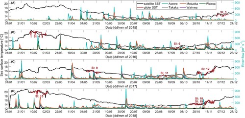
Table 1. Glider survey index, number of profiles sampled, start and end dates, seasonal affiliation, and number of LSMFs sampled for each glider survey completed in Greater Cook Strait.

Survey index	No. of profiles	Duration (days)	Start date	End date	Season	No. of LSMFs
3	2494	21	29.11.2015	19.12.2015	Spring-summer	0
4	3259	28	04.02.2016	02.03.2016	Summer	2
6	2877	24	15.09.2016	08.10.2016	Spring	2
9	3419	25	04.05.2017	28.05.2017	Autumn	2
11	3597	30	22.08.2017	20.09.2017	Winter-spring	3
12	4804	31	30.10.2017	29.11.2017	Spring	4
15	5813	33	04.02.2018	05.03.2018	Summer-autumn	9
18	6059	42	18.10.2018	28.11.2018	Spring	1
19	6364	42	18.10.2018	28.11.2018	Spring	1

Teledyne Webb Research Slocum G2 gliders used over the 3-year period were equipped with Seabird (conductivity temperature depth) CTD sensor, Aanderaa Oxygen Optode and Wet Labs Environmental Characterisation Optics (ECO) ‘puck’, that measured chlorophyll-a fluorescence, backscatter (at 470, 532, 660 and 700 nm) and chromophoric dissolved organic matter (CDOM). Temperature, conductivity, and pressure data were sampled at 0.5 Hz, and subsequently processed to remove spikes. Data were averaged in vertical bins of 1 m. Glider data processing was completed using the SOCIB glider toolbox (https://github.com/socib/glider_toolbox) (Jhugroo et al. 2020; Troupin et al. 2015) and includes correction for the thermal lag error for the unpumped CTD unit, which is standard on Slocum gliders (Garau et al. 2011).

3.1.1. Identifying low-salinity submesoscale features (LSMFs)

We used Salinity $\le 34.75$ PSU to define the maximum depth of an observed LSMF (vertical scale) for each profile. This fixed threshold was selected so as to consistently isolate as many features as possible. The mean LSMF depth of each feature was then calculated from all associated profiles. Similarly, mean mixed layer (MLD) of each LSMF was calculated from all associated profiles. LSMF depths and mixed layer depths of LSMFs were then all grouped into seasons. Further details of methods used to identify LSMFs are described in Jhugroo et al. (2020).

Mixed layer depth (MLD) was defined as the depth at which density becomes 0.125 kg m${}^{-3}$ denser than that at the ocean surface. This definition of MLD generally coincides with the seasonal thermocline (Chiswell 2011) and was introduced by Chiswell et al. (2013) while investigating the climatology of chlorophyll-a in the southwest Pacific Ocean. Due to the sampling strategies used for the glider missions, a vehicle would not always reach the surface and surface density was calculated as the mean over the upper 5 m from glider observations. At times, as the LSMF moved away from the source, gliders sampled either the edge or were outside of LSMFs, depending on currents and tides which modified the glider's path. Sampled glider transects are thus not always observing the largest gradients in the LSMF.

3.2. Vertical and lateral buoyancy gradients

Density stratification (or degree of stability) was characterised by calculation of the buoyancy frequency (sometimes known as Brunt–Väisälä frequency) squared: $N^2=-(g/{\rho }_0)(\mathrm{\partial \rho }/\mathrm{\partial z})$ where g = 9.81 m s${}^{-2}$ is the acceleration due to gravity, ${\rho }_0=1027$ kg m${}^{-3}$ is the reference density and ρ is the potential density. The along-track lateral buoyancy gradient ($M^2$) was calculated as the difference between mixed layer buoyancy (b) on consecutive glider profiles. This requires the mixed layer buoyancy be calculated as $b=g(1-\rho /{\rho }_0)$, with ρ being the mixed layer density. The ‘balanced Richardson number’, a measure of horizontal buoyancy gradient against the vertical stratification, was then calculated as $R{i}_b=(N^2{f}^2)/M^4$ where f is the Coriolis parameter and $M^2$ is the horizontal buoyancy gradient. Ri${}_b$ provides a criterion to indicate the likely occurrence of submesoscale processes (Biddle and Swart 2020; Thomas et al. 2013). As Ri${}_b$ approaches unity, or is smaller than 1 (when horizontal buoyancy gradients are larger than vertical buoyancy gradients), it indicates that destabilising submesoscale processes may occur (Biddle and Swart 2020; Thomas et al. 2013), resulting in mixed layer baroclinic instabilities and fronts.

3.3. Chlorophyll-a fluorescence quenching correction

Chlorophyll-a concentration (Chl-a) was used as a proxy of phytoplankton biomass under non-limiting environmental conditions. Chl-a values from glider observations exhibited strong light-dependent depressions each day resulting from non-photochemical quenching processes. The Chl-a from all glider missions was corrected for quenching before analysis and interpretation. While in-vivo fluorescence provides a proxy for Chl-a pigment concentration, it is sensitive to physiological downregulation under incident irradiance (fluorescence quenching; Morrison 2003; Thomalla et al. 2017, 2018). Existing methods from the literature have corrected for quenching (Behrenfeld and Boss 2003; Biermann et al. 2015; Hemsley et al. 2015; Sackmann et al. 2008; Xing et al. 2012; Swart et al. 2015). However, these methods require certain assumptions to be made that were not valid for all seasons and so requires an adaptive correction.

Quenching corrections followed the methodology provided by Thomalla et al. (2018). First, day and night profiles of Chl-a and $b_{\mathrm{bp}700}$ were partitioned according to times of local sunrise and sunset. Night profiles were averaged to create a single mean profile of Chl-a and $b_{\mathrm{bp}700}$. The vertical extent of daytime quenching (quenching depth) was determined as the depth minimum of the difference between mean night and day Chl-a within the euphotic zone (1% light depth). A preceding night's profile was used to correct the following day's quenched daytime profiles. Quenching depth was calculated as the point that marked the steepest gradient from the maximum difference in the surface (5 m) to the five smallest absolute differences and points where the difference intercepts 0. A third night profile was created as the mean ratio between Chl-a and $b_{\mathrm{bp}700}$. This third profile was then multiplied by the day $b_{\mathrm{bp}700}$ profile from the quenching depth to the surface to correct for quenching. Although quenching was observed in all seasons, it was more prominent in months when daylight hours were longer (not shown). Minimal quenching was observed during the winter months.

3.4. Satellite observations

The sea surface temperature (SST) distribution was obtained from a single-sensor multi-satellite level 3S SST product for a 144-hour period (day and night time composite), derived using observations from Advanced Very High-Resolution Radiometer (AVHRR) instruments on NOAA polar-orbiting satellites (available from 1981 onwards). Given the number of cloudy days in the region, this dataset had the best co-location of comparable data products. It is provided as a 0.02${}^{\circ }\times$ 0.02${}^{\circ }$ (2 km) cylindrical equidistant projected map over the region 144-hour average of all the highest available quality SSTs that overlap with that cell, weighted by the area of overlap. Remotely sensed SST values are skin temperature of the water body. SST timeseries was computed by choosing the mean value along a track that cuts through Greater Cook Strait spanning ${173}^{\circ }0$E to ${173}^{\circ }6$E. The sea surface chlorophyll (SSC) data used is a level 3M $9\times 9$-km 8-days composite product (available at https://oceancolor.gsfc.nasa.gov/). Similar to SST, SSC was extracted along a track that cuts through Greater Cook Strait comparable to an averaged glider mission track.

3.5. Wind and river discharges

Remote Sensing Systems Cross-Calibrated Multi-Platform (CCMP, V2) is a 6-hourly ocean wind product on 0.25 degree grid. Version 2.0 is available online at www.remss.com/measurements/ccmp and was accessed on 8 June 2020. The V2 CCMP processing combines Version-7 RSS radiometer wind speeds, QuikSCAT and ASCAT scatterometer wind vectors, moored buoy wind data and ERA-Interim model wind fields using a Variational Analysis Method. Wind time series for analysis was extracted for three locations: on land (${41}^{\circ }13$S, ${172}^{\circ }63$E), in the coastal bays (${40}^{\circ }63$S, ${173}^{\circ }13$E) and in the middle of Greater Cook Strait (${40}^{\circ }38$S, ${173}^{\circ }63$E).

Each coastal bay has freshwater contributions from two main rivers: the Aorere and Takaka Rivers discharge into Golden Bay and the Motueka and Waimea/Wairoa rivers discharge into Tasman Bay. The Wairoa River flows north for 45 kilometres before combining with the Wai-iti River to form the Waimea River. The combined rivers then flow into Tasman Bay. Gauged data of daily river flows for the five rivers above were obtained from NIWA and Tasman District Council for the period 2015 to 2018. The geographic locations of each river gauge are shown in Figure 2C.

4. Results

Four years of SST, river flow and LSMF temperatures are synthesised in Figure 3, Tables 2 and 3. There is both year-to-year variability in river flows, as well as inherent peakedness of river flows overlaid on the seasonal cycles in temperature. Against this seasonal context, we describe results relating to the detection of the LSMFs, how various LSMF properties vary with season, and the relationship between the glider in-situ data at depth and that measured at the surface by satellite.

Table 2. Seasonal SST ranges as observed from satellite and glider the period 2015–2018. Note that summer range computations comprise months December, January and February and therefore overlap between 2 years (e.g. Summer 2015 would comprise December 2015, January 2016 and February 2016).

Year	Platform	Autumn SST [${}^{\circ }$C]	Winter SST [${}^{\circ }$C]	Spring SST [${}^{\circ }$C]	Summer SST [${}^{\circ }$C]
2015	Satellite	15.4–19.4	12.5–15.8	12.7–14.5	14.6–21.3
	Glider				13.7–21.2
2016	Satellite	14.8–19.6	12.8–15.1	12.8–15.0	14.5–17.9
	Glider	19.0–19.6		12.2–14.1
2017	Satellite	15.3–17.7	13.1–15.4	13.1–18.3	12.4–21.1
	Glider	14.4–16.5	12.4–13.4	12.8–18.0	18.2–21.3
2018	Satellite	14.9–20.2	13.2–15.2	13.1–15.9
	Glider	18.5–20.6		13.5–16.2

Table 3. LSMF number (○: summer, ⊗: autumn, •: winter, ★: spring), geographical location, glider survey index (SI), sampling dates, number of profiles sampled during each LSMF, mean and standard deviation of LSMF depth, mean and standard deviation of mixed layer depth (MLD) during each LSMF and maximum chlorophyll-a concentration measured during each LSMF. LSMFs are numbered in chronological order.

LSMF No.	Location	SI	Date	Year	no. of profiles	LSMF depth [m]	MLD [m]	Max Chl-a [mg m${}^{-3}$]
1${}^{\circ }$	Farewell Spit	4	Feb, 5	2016	75	8.6 ± 2.7	7.3 ± 1.3	7.9
2${}^{\circ }$	Farewell Spit	4	Feb, 22–24	2016	139	15.4 ± 4.7	18.6 ± 4.7	2.6
3${}^{\star }$	Greater Cook Strait	6	Sep, 24–25	2016	147	31.6 ± 3.4	29.5 ± 1.5	4.4
4${}^{\star }$	Greater Cook Strait	6	Oct, 1–3	2016	275	12.1 ± 5.3	16.0 ± 6.4	3.4
5${}^{\otimes }$	Greater Cook Strait	9	May, 16–18	2017	431	22.4 ± 8.9	28.0 ± 5.1	2.1
6${}^{\otimes }$	Farewell Spit	9	May, 21–22	2017	113	22.2 ± 7.2	17.0 ± 6.1	1.6
7${}^{\bullet }$	Stephens Island	11	Aug, 30–31	2017	156	32.3 ± 5.1	29.0 ± 2.9	3.5
8${}^{\star }$	Farewell Spit	11	Sep, 3–4	2017	159	14.7 ± 4.8	22.0 ± 3.5	1.5
9${}^{\star }$	Greater Cook Strait	11	Sep, 10–11	2017	76	17.6 ± 4.1	21.0 ± 4.9	4.0
10${}^{\star }$	The bays	12	Oct, 30–31	2017	128	21.9 ± 8.1	9.0 ± 2.1	3.0
11${}^{\star }$	Greater Cook Strait	12	Oct, 31 -- Nov, 1	2017	270	11.8 ± 4.6	7.0 ± 2.2	2.8
12${}^{\star }$	Greater Cook Strait	12	Nov, 4–5	2017	248	28.1 ± 6.2	25.0 ± 4.8	3.7
13${}^{\star }$	The bays	12	Nov, 26–29	2017	715	24.6 ± 5.8	9.0 ± 4.0	3.9
14${}^{\circ }$	The bays	15	Feb, 5–6	2018	320	20.2 ± 13.5	28.0 ± 6.9	3.3
15${}^{\circ }$	Greater Cook Strait	15	Feb, 15–16	2018	238	6.9 ± 2.3	6.0 ± 2.0	3.0
16${}^{\circ }$	Farewell Spit	15	Feb, 18–19	2018	151	9.9 ± 3.6	11.0 ± 3.9	3.7
17${}^{\circ }$	Farewell Spit	15	Feb, 20	2018	47	7.3 ± 2.3	15.5 ± 6.4	2.3
18${}^{\circ }$	Farewell Spit	15	Feb, 24–25	2018	111	28.3 ± 6.0	27.0 ± 3.4	1.5
19${}^{\otimes }$	The bays	15	Mar, 1	2018	15	2.5 ± 0.5	10.0 ± 1.5	1.2
20${}^{\otimes }$	The bays	15	Mar, 1–2	2018	89	3.5 ± 1.2	8.0 ± 1.5	1.3
21${}^{\otimes }$	The bays	15	Mar, 2	2018	117	6.6 ± 2.9	12.0 ± 4.4	3.4
22${}^{\otimes }$	The bays	15	Mar, 3–5	2018	654	17.5 ± 8.5	7.0 ± 2.5	4.3
23${}^{\star }$	Greater Cook Strait	18	Oct, 24–26	2018	371	13.3 ± 10.6	16.0 ± 4.8	3.3
24${}^{\star }$	Greater Cook Strait	19	Nov, 7–9	2018	309	15.3 ± 3.3	17.0 ± 3.2	4.3

4.1. River discharge variability and ex-tropical cyclone extrema

River flows are inherently highly event-driven and the variability in the resulting oceanic buoyancy inputs at the coastal margin underpins LSMFs development. Aorere and Motueka Rivers had the highest river discharges into the coastal bays compared to Takaka, Waimea and Wairoa Rivers (Figure 3 and Table 4). In 2015 and 2016, Aorere River had the highest contribution in river discharge into the bays with annual-mean river flows of 60.0 m${}^3$ s${}^{-1}$ and 83.9 m${}^3$ s${}^{-1}$ respectively. In 2017 and 2018, Motueka River had the highest contribution with annual-mean river flows of 68.6 m${}^3$ s${}^{-1}$ and 70.3 m${}^3$ s${}^{-1}$ respectively. Seasonally, river discharge was highest in Austral winter compared to other seasons for all five rivers (Table 4). The two larger rivers, Aorere and Motueka, experienced their lowest discharge in summer while the three smaller rivers, Takaka, Waimea and Wairoa, had discharge minima during spring (Table 4).

Table 4. Seasonal mean of river flow for each river discharging into Golden and Tasman Bays over the period 2015–2018.

	Summer river flow [m${}^3$ s${}^{-1}$]	Autumn river flow [m${}^3$ s${}^{-1}$]	Winter river flow [m${}^3$ s${}^{-1}$]	Spring river flow [m${}^3$ s${}^{-1}$]
Aorere	59.44	69.24	87.72	63.63
Takaka	29.17	32.71	45.31	27.26
Motueka	51.73	62.44	88.69	64.05
Waimea	20.93	21.46	27.09	17.35
Wairoa	18.74	17.82	21.05	14.27

However, two ex-tropical cyclones affected Greater Cook Strait during February 2018. Maximum intensity of ex-tropical cyclones Fehi and Gita on the coastal system occurred on 1 February and 20 February 2018 respectively. Rainfall associated was characterised as above normal (120–149% of average) or well above normal ($>149$% of average) across central New Zealand during February (Monthly Climate Summary 2018). Rainfall totals near Golden and Tasman Bays were 300–400% of the monthly normal (Monthly Climate Summary 2018). Post ex-tropical cyclone Fehi during the first week of February 2018, Aorere River had the highest river flow, followed by Takaka River (Table 4).

4.2. Detection of LSMFs

Observations from glider surveys identified 24 persistent LSMFs (Table 3, Figure 4). Seasonally, there were 7 LSMFs in summer, 6 in autumn, 1 in winter and 10 in spring. The total number of profiles sampled during LSMFs for each season were 1081 in summer, 1419 in autumn, 156 in winter and 2698 in spring. Geographically, seven LSMFs were observed north of Farewell Spit, nine in Greater Cook Strait, one near Stephens Island and seven in Golden and Tasman Bays. LSMFs were observed in all seasons and in every survey, with the exception of the November–December 2015 glider survey (Survey 3, Figure 4A). More LSMFs were also observed during the summer 2018 glider survey (Figure 4G). The LSMFs were observed within the top 50 m of the water column profiles, indicating that these features are not restricted to the surface. Twenty of the LSMFs were detected after increased river flows (Figure 3), leaving four LSMFs observed in the absence of direct riverine inputs. LSMF 23 was more saline than most other LSMFs, while LSMFs 10 and 13 were sampled in Golden and Tasman bays. This suggests that some of the detected LSMFs could be a result of long residence times as opposed to a direct initiation from increased river flows.

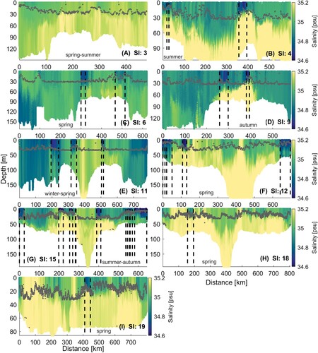
Figure 4. A–I, Salinity transects for nine glider surveys in Greater Cook Strait (SI = survey indices). Start and end of LSMFs as identified from the glider data (see Section 3.1.1) are highlighted by black dashed lines in each transect. Mixed layer depth is overlayed as grey scatter for each survey. Additional details are listed in Tables 1 and 3.

In Greater Cook Strait, when river inflows were significant and northwards wind strength was weak, the lag between river flow and measured LSMF offshore was largest (∼2–3 weeks, e.g. Figure 5B and D). When river flows exceeded 600 m${}^3$ s${}^{-1}$, LSMFs did not require external drivers (e.g. wind or tide) to be advected offshore. For strong winds and large river inflows, wind enhances offshore advection of LSMFs and the lag timescale between river flow and observed LSMFs was relatively short (e.g. Figure 5A and C). Figures 5E and G show the alternate response of LSMFs when river flows are $<600$ m${}^3$ s${}^{-1}$ and strong winds persist. In the presence of cyclones, increased wind strength and increased precipitation lead to large quantities of buoyant river water being advected offshore much faster. Smaller lags between river flow and offshore LSMFs occur after extreme events ( Figures 5J and L).

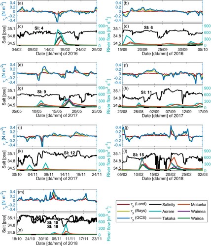
Figure 5. A,B,E,F,I,J,M, Time series of wind stress over land (red), Golden and Tasman Bays (yellow) and Greater Cook Strait (blue) for the length of each glider surveys 4, 6, 9, 11, 12, 15, 18 and 19 respectively. C,D,G,H,K,L,N River flow timeseries of Aorere (blue), Takaka (grey), Motueka (orange), Waimea (purple) and Wairoa (green) Rivers over the period of each glider survey. C,D,G,H,K,L,N Glider salinity timeseries at 8 m for each glider survey respectively (black line). C,D,G,H,K,L,N Dots on the time-axis scale indicate dates on which LSMFs were sampled by glider; green dots for LSMFs sampled inside Golden and Tasman bays and black dots for LSMFs sampled outside the bays.

4.3. Seasonal variability of LSMFs

Figure 7 shows that LSMF temperature signals tend to follow the seasonal trend; warmer in summer and colder in winter. LSMF seasonal characteristics were compared to ambient shelf conditions (Figure 6). Typically, LSMFs tend to be characterised by higher temperatures than the seasonal means for each season, with the difference being more pronounced in summer and autumn.

Figure 6. Seasonal mean of all profiles (black) and LSMF profiles (blue) of temperature (first column), salinity (second column), density (third column), CDOM (fourth column) and chlorophyll-a concentration (last column). Shaded regions represent standard deviation around each corresponding mean profile.

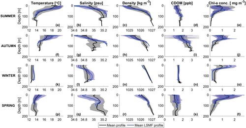
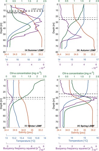
Figure 7. Profiles of salinity (orange), Chl-a (green), temperature (blue), buoyancy frequency squared (purple) for A, summer 2017–18, LSMF 16, B, autumn 2017, LSMF 5, C, winter 2017, LSMF 7 and D, spring 2017, LSMF 12. Grey and black dashed lines indicate mean LSMF depth and mixed layer depth respectively. Averaging was performed over A, 151 profiles during LSMF 16, B, 431 profiles during LSMF 5, C, 156 profiles during LSMF 7 and D, 248 profiles during LSMF 12. Note that temperature scale was adjusted in each subplot due to seasonal variability.

4.3.1. Summer

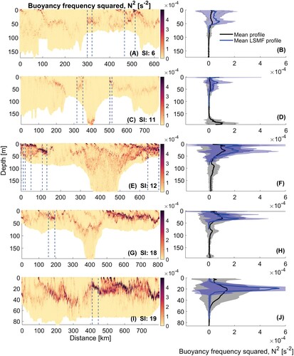
Summer LSMFs depths were shallower compared to other seasons (Figure 7), with median depth 10 m, but also had the most variability with LSMF depth between 0 and 37 m. In summer, MLD of LSMFs had median 13 m and varied in the range 5–35 m. Variability in MLD of LSMFs was large in summer, with high temperatures resulting in strong stratification with N${}^2$ reaching ${10}^{-3}$ s${}^{-2}$ ( Figures 8A and C). In open ocean conditions, submesoscale motions are often weaker in summer when MLDs are shallow, yet we observed numerous LSMFs during summer. Of note, Greater Cook Strait is a shallow shelf region persistently impacted by tidal straining, strong winds, residual tidal currents, upwelling and diurnal cooling. Moreover, Somavilla et al. (2017) have shown that surface warming is not definitively linked to a more stratified ocean with shallower mixed layers.

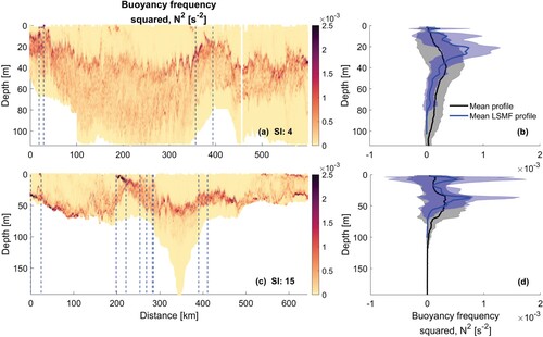
Figure 8. A,C, Buoyancy frequency squared transects for glider surveys in summer. Start and end of summer LSMFs as sampled by glider denoted by dashed lines. B,D, Mean of all profiles for each summer glider survey (black) and summer LSMF profiles (blue) of buoyancy frequency squared within each survey, with shaded regions representing standard deviation around the mean.

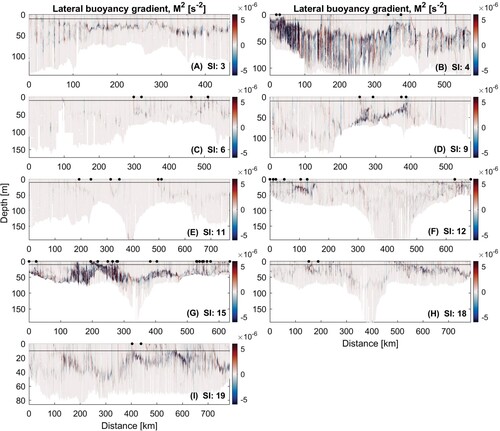
Lateral buoyancy gradients observed in summer were stronger than the other seasons (Figure 9B and G), promoting submesoscale activity. Summer LSMFs had the strongest lateral buoyancy gradients with mean M${}^2$ on the order of ${10}^{-6}$ s${}^{-2}$ at the fronts on the edges of LSMFs ( Figures 9B, D and G). More LSMFs and generally less saline waters in the bays were observed in February–March 2018 (SI:15, Figure 4G). Summer also saw subsurface Chl-a maxima and higher variability in ambient shelf salinity.

Figure 9. A–I, Lateral buoyancy gradients for each glider survey. Start and end of each LSMF as sampled by glider denoted by black dots. Grey solid line indicates the depth to which density was interpolated horizontally across profiles with missing shallow values, due to the glider diving pattern.

Significant year-to-year variability was evident across the observed summers in both LSMFs and ambient shelf sea. Summer 2017–18 was much warmer (Figure 3D) than other summers over the period 2015–2018 due to the La Niña event (2017–18) as reported by Monthly Climate Summary (2018). A marine heatwave was large and persistent, while three ex-tropical cyclones affected New Zealand coastlines (Monthly Climate Summary 2018). February 2018 was an anomalous summer with above average rainfall and SST anomalies of up to 5${}^{\circ }$C.

4.3.2. Autumn

Ocean preconditioning by ex-tropical Cyclones Fehi and Gita skewed the LSMFs observed by a glider during survey 15 in Autumn. These weather events induced shallower MLDs, and more outliers in MLD of LSMFs in autumn. LSMFs during autumn exhibited high temperatures, higher variability in ambient shelf salinity, and stratification N${}^2$ reaching values $>5\times {10}^{-4}$ s${}^{-2}$. MLD of LSMFs were shallower but highly variable in autumn compared to other seasons. In terms of biological response, surface Chl-a maxima and high variability in CDOM were observed.

4.3.3. Winter

There was only one winter survey over the 2015–2018 period which, while it has implications for the interpretation of seasonality of LSMFs, it still provides valuable information on winter LSMFs. The winter LSMFs had no temperature differential and it had a 20 m deeper LSMF depth and MLD (Figure 7C). It was also characterised by an increase in surface Chl-a compared to ambient waters and consistent CDOM. Stratification in winter was, as expected, weaker than other seasons, and an order of magnitude weaker than summer stratification, with N${}^2<2\times {10}^{-4}$ s${}^{-2}$. Winter LSMFs extended much deeper into the subsurface, with median depth 32 m, and had the least variability (22–48 m). A consequence was the deepest MLD was also observed in a winter LSMF (Figure 7). Furthermore, winter lateral buoyancy gradients were generally weaker ( Figures 9B and G), in winter with mean M${}^2$ on the order of ${10}^{-8}$ s${}^{-2}$, small compared to other LSMFs. However, the gradient were still identifiable (Figure 9E). In comparison to other seasons, the winter survey observed weaker vertical and horizontal gradients. In addition it revealed how the presence of an LSMF can considerably alter the ambient stratification and stabilise the water column dominating the system during a period of pre-existing weak gradients. This can sustain local primary production during a period when MLD were deepest and frequency of extreme upwelling is low (Chiswell et al. 2016).

4.3.4. Spring

Spring LSMFs had median depths of 20 m, but varied from the surface to 39 m (Figure 12A). Mean lateral gradients of spring LSMFS had observed M${}^2$ on the order of ${10}^{-7}$ s${}^{-2}$ at the fronts (Figure 9C–I). In terms of biological processes spring typically supported subsurface Chl-a maxima. Glider surveys also straddled the seasons (at the beginning, end or in the middle of a season) and revealed that intra-seasonal stratification variability is also apparent amongst LSMFs. For example, stratification is weaker at the beginning of spring in September compared to end of spring in November (Figure 10C and E).

Figure 10. A,C,E,G,I, Buoyancy frequency squared transects for glider surveys in spring. Start and end of spring LSMF as sampled by glider denoted by dashed lines. B,D,F,H,J, Mean of all profiles for entire glider surveys (black) and LSMF profiles (blue) of buoyancy frequency squared, with shaded regions representing standard deviation around the mean.

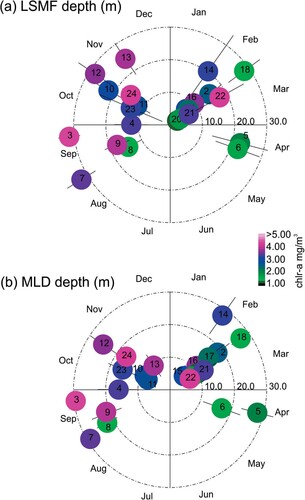
Figure 12 provides a synthesis of LSMF depth and mixed layer depths for all seasons with their Chl-a level, while at the same time illustrating the gaps in seasonal coverage. Both the LSMF and MLD values result in consistent seasonal distributions but with clear event-to-event differences in LSMF and MLD.

4.4. Comparisons of in-situ and remote observations

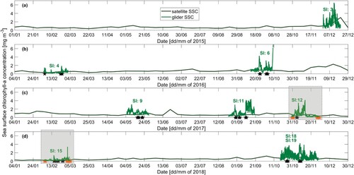
Satellites SST and SSC were compared to gliders SST and SSC over the period 2015–2018 (Figure 3) to place the glider measurements in a broader, continuous context, while the seasonal SST ranges are reported in Table 2. The relatively warm range in autumn 2018 is because glider profiles were sampled at the beginning of autumn in March 2018, when the ocean was warmed from summer 2017 to 2018. Summers 2015–2016 and 2017–2018 were warmer than summer 2016–2017 by $\sim {3.3}^{\circ }$C. Winter SST ranges were similar throughout the 2015–2018 period. In 2017, SST range was the smallest in autumn while SST range was the largest in spring compared to other years. Satellite and glider SSC were generally low and compared well in summer 2015–2016 and summer 2017–2018 (Surveys 4 and 15; Figure 11B and D).

Figure 11. Satellite and glider sea surface chlorophyll (SSC) timeseries for A, 2015, B, 2016, C, 2017 and D, 2018. Surface value of Chl-a for glider observations was taken as the mean Chl-a value of top 8 m due to glider's diving pattern. Stars indicate dates on which LSMFs were sampled by glider; orange stars for LSMFs sampled inside Golden and Tasman bays and black stars for LSMFs sampled outside the bays. C,D, Shaded boxes highlight the two scenarios chosen for satellite and glider sea surface chlorophyll comparison.

Greater Cook Strait satellite observations are close to weekly temporal resolution. Generally satellite SST and glider SST compared well at the 6-day period, confirming that satellite is a reliable platform for SST variability analysis. However, localised variability captured by the glider during events such as upwelling or presence of LSMF, was not seen in satellite SST and SSC. This is because temporal and spatial resolution were different for the satellite products and gliders. As such, for the satellite SST product, much of the variability is averaged over space (geographical line spanning ${173}^{\circ }0$E to ${173}^{\circ }6$E; $\sim 50$ km) and time (144 hours). Similarly, the satellite SSC 9-km 8-day composite product is an average over space and time (Figure 11). Glider SST and SSC varied locally in space and time while satellite SST and SSC, as plotted on Figure 3, represent a mean over a transect comparable to an averaged glider track.

4.5. Surface versus subsurface chlorophyll-a in LSMFs

Subsurface Chl-a maxima in LSMFs was observed during spring and summer, while winter and autumn Chl-a maxima were evident at the surface. To examine the different data streams, two scenarios of surface and subsurface LSMF Chl-a were compared: (1) when satellite and glider SSC compared well for LSMF 16 in summer 2017–18 (SI: 15) and (2) when satellite and glider SSC were different for LSMF 12 in spring 2017 (SI: 12). In both scenarios, subsurface Chl-a was higher than surface Chl-a (Figure 7A and D). These two glider surveys were selected as PAR was available, which permitted robust quenching correction of Chl-a observations. Glider Chl-a measurements were averaged over 5813 profiles during survey 15 and over 4804 profiles during survey 12, while the satellite product is a 9-km 8-day composite and was evaluated as a mean over a geographical location for this study. The spatial averaging the implies an underestimate in Chl-a should be expected from the remotely sensed product.

5. Discussion

LSMFs are ubiquitous throughout the annual cycle in Greater Cook Strait. The impact of LSMFs on baroclinic variability and stratification varies with season and the associated seasonality in river discharges. Extreme weather events are overlaid on seasonal dynamics which significantly modulate wind stress, ocean temperatures and tidal straining (Figure 1). Geographically, LSMFs were detected in four main regions: Farewell Spit, directly north of the coastal bays in Greater Cook Strait, Stephens Island (eastern side of Greater Cook Strait) and the coastal bays (Figure 2D). Potential mechanisms responsible for this geographical spread are:

(1)	Strength of residual flows in the coastal bays (Chiswell et al. 2019).
(2)	Quantities of riverine inputs and relative contributions from each river, noting that Aorere and Motueka have the biggest river contributions in the coastal bays (Figure 3).
(3)	Wind strength and direction (Chiswell et al. 2019; Jhugroo et al. 2020).
(4)	Presence and strength of the coastal d'Urville Current (Jhugroo et al. 2020).

5.1. LSMFs seasonal variability

Seasonality of river flows from small mountainous rivers highlights winter discharges are typically greater than the other three seasons (Goñi et al. 2013; Oosterbaan 1994). Similar conditions were prevalent in Greater Cook Strait whereby river flows was higher in winter (Figure 3, Table 4). These results suggest higher freshwater flow is likely to lead to increased occurrence of LSMFs in winter, albeit as shorter-lived events due to amplified wind mixing. Glider surveys toward the end of autumn and at the beginning of spring already favour these characteristics for winter LSMFs.

Spring, summer and autumn LSMFs were statistically well sampled. During these three seasons, LSMFs were generally 1–2${}^{\circ }$C warmer than the seasonal mean (Figures 6A,F,K,P). Fresher and warmer LSMFs were more evident in summer and autumn. SST could potentially be used as an indicator for LSMFs in these seasons. However, due to the spatial structure and ephemeral nature of LSMFs, they are often unresolved in composite satellite products since variability is smoothed out in the averaged-data or simply not observed (Figure 3). Satellite products are also impacted by cloud cover. Moreover, the summer and autumn LSMFs in this study are skewed by the increased occurrence of LSMFs during February 2018 and March 2018. Summer 2017–2018 was much warmer than summer 2015–16 and 2016–17 as that was the last time there was a La Niña event (Monthly Climate Summary 2018). The event also coincided with a marine heatwave and three ex-tropical cyclones near New Zealand coastlines (Monthly Climate Summary 2018) with subsequent increases in vertical temperature and salinity gradients.

Few studies have observed the annual and seasonal variability of the MLD and their implications for primary productivity from hydrographic profiles (e.g. Condie and Dunn 2006; d'Ortenzio et al. 2005; Guo et al. 2017; Kara et al. 2003). In this study, the seasonality in vertical structure of eddies at the submesoscale was investigated. Generally, MLD of LSMFs and LSMF depths do not always coincide. MLD was calculated from density, which is also temperature dependent, whereas LSMF depth solely depends on salinity gradients. In winter, there is less temperature variability (Figure 6K), and as a result, LSMF depths and MLD of LSMFs were more comparable (Figure 12). However, this does not hold true for summer and early autumn when temperature contributions to density are higher.

Figure 12. Synthesis of seasonal variability results showing A, LSMF depth and B, mixed layer depth. The realisations are scaled by colour representing the chlorophyll-a and the radial bar reflects the variability in each realisation.

The effects of stratifying, de-stratifying and re-stratifying events from mesoscale eddies on modulating the MLD have been examined by Stevens C et al. (2011), Bachman et al. (2017) and Gaube and Moulin (2019). Vertical extent of mixing depends on stratification, but also on wind-driven divergence and buoyancy losses. These mechanisms can compensate for and outpace the effects of ocean warming and increasing stratification on MLD (Somavilla et al. 2017). LSMFs create sustained lateral and vertical gradients in salinity in Greater Cook Strait, which in turn impact density stratification over the continental shelf region (Jhugroo et al. 2020). LSMF-induced stratification and its erosion, including their strength, timing, and relative contributions of salinity and temperature were found to be variable over different seasons. In summer and beginning of autumn, there is much stronger stratification compared to winter (Figure 8). As the ocean warms closer to summer, this trend in stratification stands out from this study.

Broadly, during summer the upper ocean is very stable due to heating leading to warmer surface temperatures and strong vertical gradients (Somavilla et al. 2017). The strong gradients are further amplified during marine heatwaves. Regularly, during warmer months, double stratification maxima were observed (e.g. Figures 8C, D and 10E, F). In these instances, one stratification maximum was observed near-surface and another one in the subsurface. These were caused by the near-surface temperature stratified layer and subsurface salinity stratified layer respectively. The addition of freshwater from LSMFs makes the upper ocean even more buoyant and stable, and harder to mix and destabilise. Stronger drivers are required to destabilise and mix the water column.

5.2. Biophysical connections in LSMFs

The lag between river discharge events and appearance of measured LSMFs offshore was found to vary between 2 and 27 days (Figure 5). This lag was dependent on factors such as amount of river flow, wind strength, residual tidal flow and presence of extreme events such as cyclones or marine heatwaves. Seasonality of the system can amplify or dampen each of these forcing mechanisms. February is usually the warmest and driest month of the year in New Zealand, while July the coldest and wettest (Monthly Climate Summary 2018). As a result, river discharge tends to be higher during winter and lower in summer. This is common in temperate regions (Lancelot and Muylaert 2011). Jhugroo et al. (2020) reported that LSMFs are advected out of the coastal bays by a combination of river water saturation in the bays, residual northward tidal flows, and strong northwards wind in the bays. Wind can enhance advection of LSMFs for 38% of the time in spring (Jhugroo et al. 2020). The time lag range of 2–27 days provides an indicative timescale for nutrient cycling in LSMFs as they advect seawards from the land-sea boundary. Understanding causal relationships between riverine nutrient supply to coastal and oceanic waters is important for determining ecosystem responses and time frames (Justić et al. 1993).

Subsurface Chl-a maxima development often occurs in stratified coastal waters which are significant for global biogeochemical cycling and trophic budgets (Barnett et al. 2019). Better understanding of subsurface Chl-a maxima dynamics and their controls in shelf seas is required for global trophic budgeting efforts to realistically represent the range of ecosystem behaviours. During warmer months, water masses in this shallow shelf sea warm faster creating a temperature stratified layer near the surface. MLD follows the near-surface stratification peak as it is calculated from density. The subsurface Chl-a maximum layer was observed closer to the salinity stratified layer at the base of LSMFs. Subsurface Chl-a maxima were observed in late summer 2018 (e.g. Figure 7A) and spring 2017 LSMFs (e.g. Figure 7D). LSMFs during these two seasons (summer and spring) are characterised by temperature gradients increasing stratification near the surface while salinity gradients modified subsurface increase stratification in the subsurface (Figure 7). It is worth noting that LSMFs are considered to have been sampled at different stages of their evolution from the land-sea boundary. Since LSMFs start off near the coastline and are advected well offshore by the time they are observed with glider surveys, a subsurface Chl-a maximum is an expected feature of stratified systems. This is likely due to evolution of the surface layer nutrient environment over time. This finding emphasises the role of LSMFs on stratification and the biological response in austral spring and summer. Observations of subsurface Chl-a maxima are particularly valuable since efforts, to date, have examined phytoplankton blooms either in horizontal surface variability or depth-integrated Chl-a, ignoring potential changes in vertical structure (Chiswell et al. 2015).

5.3. Do high rainfall weather events influence LSMF occurrence?

With rivers being a major factor spawning LSMF it is important to consider future projections. Up until recently there has been no detectable change in the frequency of extreme weather events in long-term trends for the west coast of Aotearoa New Zealand. However, extreme events are becoming warmer (Chiswell and O'Callaghan 2021).

Previous studies have shown that many small mountainous rivers are affected by periodic to aperiodic intense precipitation events such as monsoonal activity, La Niña and El Niño phases of the El Niño-Southern Oscillation (ENSO), tectonic activity and tropical cyclonic activity (Goldsmith et al. 2008). The presence of extreme events resulting in cyclones, increased rainfall and thus, river discharge, led to more frequent and fresher LSMFs in Greater Cook Strait (Figure 4G). Typically, the summer season is when LSMFs would be less frequent due to lower rainfall (Monthly Climate Summary 2018) and relatively minimal river discharges (Table 4).

Rainfall associated with ex-tropical cyclones translating southwards from the tropical Pacific fuelled by warmer oceans is changing summer discharges around Aotearoa New Zealand. After ex-Tropical Cyclone Fehi during the first week of February 2018, Golden Bay was more impacted than Tasman Bay due to high discharges from Aorere and Takaka Rivers. After ex-Tropical Cyclone Gita, both bays were impacted by high discharges from Motueka, Aorere and Takaka Rivers. Throughout the year, Aorere and Motueka Rivers have the highest discharges into the bays (Figure 3 and Table 4). However, this study found that Takaka River is more responsive to extreme events, with its discharge comparable to Aoerere and Motueka after the 2018 cyclones. Examples of other small mountainous rivers vulnerable to extreme events include Taiwan rivers (Goldsmith et al. 2008; Kao et al. 2011) and Galabre River in the Rhône River catchment (Navratil et al. 2011).

A distinctive characteristic of small mountainous rivers is that the movement of water and associated material from land to the coastal ocean is event-dominated and occurs on time scales of hours to days (Wheatcroft et al. 1997, 2010). Discharge peaks often coincide with specific coastal oceanic conditions, such as elevated wave energy or winds from a certain direction (Harris CK et al. 2005). For example, this study demonstrated that when river flow is strong enough and northwards wind strength is weak, the lag between river flow and measured LSMF offshore is largest (Figure 5). A minimum threshold of 600 m${}^3$ s${}^{-1}$ is required for LSMFs to advect offshore without external drivers. Wind enhances offshore advection of LSMFs, reducing the lag between river flow and measured LSMFs. Presence of cyclones lead to increased wind strength and increased precipitation which causes large quantities of buoyant river water being advected offshore much faster ( Figures 5J and L).

5.4. Conclusion

Over 38,000 CTD profiles from nine ocean glider missions enable a shift in perspective to look at event-based impacts of rainfall on stratification and phytoplankton in a shelf sea region of Aotearoa New Zealand. Autonomous technology complemented remote sensed data to provide a significant boost in data density and knowledge of mean and extreme discharge events across seasons, which generated LSMFs and subsurface Chl-a. Following the LSMFs showed the buoyancy flux evolved to drive upper ocean submesoscale variability and enable a criterion to be developed for production of LSMFs. While there are sufficient data to enable a broad description of the seasonal variability of LSMFs, additional glider surveys in winter, and in a wider range of locations, would enable greater understanding about the transition from winter to spring and associated biological dynamics ahead of the spring bloom.

Acknowledgments

KJ thanks Stefan Jendersie and Rafael Costa Santana for valuable inputs and discussions. The authors thank Fiona Elliott for her contribution to glider-related field work, and also acknowledge the help of Nelson fishing charters in glider deployments and recoveries. KJ and JMOC collected the data. KJ processed and analysed the data, and wrote the initial manuscript based on her PhD work. KJ, JMOC and CLS contributed to interpretation of the results. JMOC and CLS finalised the manuscript. All authors read and approved the submitted version.

Data availability statement

Glider data are publicly available through the SEANOE data depository (O'Callaghan and Elliott 2020). The SST product is available via the Australian Ocean Data Network (AODN) portal under the Integrated Marine Observing System (IMOS) (https://portal.aodn.org.au/search). Further information on the product and its processing is available at https://catalogue-imos.aodn.org.au/geonetwork/srv/eng/metadata.show?uuid=34110d06-707b-4f73-970e-9b38e9fcb7da. SSC data available at https://oceancolor.gsfc.nasa.gov/. Remote Sensing Systems Cross-Calibrated Multi-Platform (CCMP) 6-hourly ocean vector wind analysis product available online at www.remss.com/measurements/ccmp. Gauge measurements of daily river flow were obtained from NIWA and Tasman District Council.

Disclosure statement

No potential conflict of interest was reported by the author(s).

Additional information

Funding

This research was funded by Sustainable Seas Stressor Footprints Project 4.2.2, Marsden Fund Projects 17-NIW-010 and 21-NIW-024, and NIWA Strategic Science Investment Fund (SSIF) Flows and Productivity Programme. River flow data for Aorere at Devils Boots (site 52003) is funded by NIWA and for Takaka at Kotinga (site 52901), Motueka at Woodmans Bend (site 57015), Waimea at Tasman District Council Nursery (site 57523) and Wairoa at Gorge 2 (site 57525) are funded by Tasman District Council and MBIE Marine Science SSIF Platform[OCOF2301].

References

- Bachman SD, Taylor J, Adams K, Hosegood P. 2017. Mesoscale and submesoscale effects on mixed layer depth in the Southern Ocean. J Phys Oceanogr. 47:2173–2188. doi: 10.1175/JPO-D-17-0034.1.
- Barnett ML, Kemp AE, Hickman AE, Purdie DA. 2019. Shelf sea subsurface chlorophyll maximum thin layers have a distinct phytoplankton community structure. Cont Shelf Res. 174:140–157. doi: 10.1016/j.csr.2018.12.007.
- Behrenfeld MJ, Boss E. 2003. The beam attenuation to chlorophyll ratio: an optical index of phytoplankton physiology in the surface ocean? Deep Sea Res Part I Oceanogr Res Pap. 50:1537–1549. doi: 10.1016/j.dsr.2003.09.002.
- Biddle L, Swart S. 2020. The observed seasonal cycle of submesoscale processes in the Antarctic marginal ice zone. J Geophys Res Oceans. 47. doi: 10.1029/2019JC015587.
- Biermann L, Guinet C, Bester MN, Brierley A, Boehme L. 2015. An alternative method for correcting fluorescence quenching. Ocean Sci. 11:83–91. doi: 10.5194/os-11-83-2015.
- Cahill ML, Middleton JH, Stanton BR. 1991. Coastal-trapped waves on the west coast of South Island, New Zealand. J Phys Oceanogr. 21:541–557. doi: 10.1175/1520-0485(1991)021¡0541:CTWOTW¿2.0.CO;2.
- Carey AE, Nezat CA, Lyons WB, Kao S -J, Hicks DM, Owen JS. 2002. Trace metal fluxes to the ocean: the importance of high-standing oceanic islands. Geophys Res Lett. 29:14–1. doi: 10.1029/2002GL015690.
- Chiswell SM. 2011. Annual cycles and spring blooms in phytoplankton: don't abandon Sverdrup completely. Mar Ecol Prog Ser. 443:39–50. doi: 10.3354/meps09453.
- Chiswell SM, Bostock HC, Sutton PJ, Williams MJ. 2015. Physical oceanography of the deep seas around New Zealand: a review. N Z J Mar Freshw Res. 49:286–317. doi: 10.1080/00288330.2014.992918.
- Chiswell SM, Bradford-Grieve J, Hadfield MG, Kennan SC. 2013. Climatology of surface chlorophyll a, autumn-winter and spring blooms in the southwest Pacific Ocean. J Geophys Res Oceans. 118:1003–1018. doi: 10.1002/jgrc.20088.
- Chiswell SM, Calil PH, Boyd PW. 2015. Spring blooms and annual cycles of phytoplankton: a unified perspective. J Plankton Res. 37:500–508. doi: 10.1093/plankt/fbv021.
- Chiswell SM, O'Callaghan JM. 2021. Long-term trends in the frequency and magnitude of upwelling along the West Coast of the South Island, New Zealand, and the impact on primary production. N Z J Mar Freshw Res. 55(1):177–198. doi: 10.1080/00288330.2020.1865416.
- Chiswell SM, Stevens CL, Macdonald HS, Grant BS, Price O. 2019. Circulation in Tasman-Golden Bays and Greater Cook Strait, New Zealand. N Z J Mar Freshw Res. 55(1):223–248. doi: 10.1080/00288330.2019.1698622.
- Chiswell SM, Zeldis JR, Hadfield MG, Pinkerton MH. 2016. Wind-driven upwelling and surface chlorophyll blooms in Greater Cook Strait. N Z J Mar Freshw Res. 51(4):465–489. doi: 10.1080/00288330.2016.1260606.
- Condie SA, Dunn JR. 2006. Seasonal characteristics of the surface mixed layer in the Australasian region: implications for primary production regimes and biogeography. Mar Freshw Res. 57:569–590. doi: 10.1071/MF06009.
- Cornelisen CD, Gillespie PA, Kirs M, Young RG, Forrest RW, Barter PJ, Knight BR, Harwood VJ. 2011. Motueka River plume facilitates transport of ruminant faecal contaminants into shellfish growing waters, Tasman Bay, New Zealand. N Z J Mar Freshw Res. 45:477–495. doi: 10.1080/00288330.2011.587822.
- d'Ortenzio F, Iudicone D, de Boyer Montegut C, Testor P, Antoine D, Marullo S, Santoleri R, Madec G. 2005. Seasonal variability of the mixed layer depth in the Mediterranean Sea as derived from in situ profiles. Geophys Res Lett. 32:L12605. doi: 10.1029/2005GL022463.
- Fox-Kemper B, Ferrari R, Hallberg R. 2008. Parameterization of mixed layer eddies. Part I: theory and diagnosis. J Phys Oceanogr. 38:1145–1165. doi: 10.1175/2007JPO3792.1.
- Garau B, Ruiz S, Zhang WG, Pascual A, Heslop E, Kerfoot J, Tintoré J. 2011. Thermal lag correction on Slocum CTD glider data. J Atmosph Ocean Technol. 28:1065–1071. doi: 10.1175/JTECH-D-10-05030.1.
- Gaube P, Moulin AJ. 2019. Mesoscale eddies modulate mixed layer depth globally. Geophys Res Lett. 46:1505–1512. doi: 10.1029/2018GL080006.
- Goldsmith ST, Carey AE, Lyons WB, Kao S -J, Lee T -Y, Chen J. 2008. Extreme storm events, landscape denudation, and carbon sequestration: Typhoon Mindulle, Choshui River, Taiwan. Geology. 36:483–486. doi: 10.1130/G24624A.1.
- Gommenginger C, Chapron B, Hogg A, Buckingham C, Fox-Kemper B, Eriksson L, Soulat F, Ubelmann C, Ocampo-Torres F, Nardelli BB, et al. 2019. SEASTAR: a mission to study ocean submesoscale dynamics and small-scale atmosphere-ocean processes in coastal, shelf and polar seas. Front Mar Sci. 6:457. doi: 10.13140/RG.2.2.20415.61601.
- Goñi MA, Hatten JA, Wheatcroft RA, Borgeld JC. 2013. Particulate organic matter export by two contrasting small mountainous rivers from the Pacific Northwest, USA. J Geophys Res Biogeosci. 118:112–134. doi: 10.1002/jgrg.v118.1.
- Guo M, Xiu P, Li S, Chai F, Xue H, Zhou K, Dai M. 2017. Seasonal variability and mechanisms regulating chlorophyll distribution in mesoscale eddies in the South China Sea. J Geophys Res Oceans. 122:5329–5347. doi: 10.1002/jgrc.v122.7.
- Hadfield MG, Stevens CL. 2020. A modelling synthesis of the volume flux through Cook Strait. N Z J Mar Freshw Res. 55(1):65–93. doi: 10.1080/00288330.2020.1784963.
- Harris CK, Traykovski PA, Geyer WR. 2005. Flood dispersal and deposition by near-bed gravitational sediment flows and oceanographic transport: a numerical modeling study of the Eel River shelf, Northern California. J Geophys Res Oceans. 110:C09025. doi: 10.1029/2004JC002727.
- Harris TFW. 1990. Greater cook strait: form and flow, DSIR marine and freshwater. https://books.google.co.uk/books/about/Greater_Cook_Strait.html?id=BeeAAAAAMAAJ&pgis=1.
- Hemsley VS, Smyth TJ, Martin AP, Frajka-Williams E, Thompson AF, Damerell G, Painter SC. 2015. Estimating oceanic primary production using vertical irradiance and chlorophyll profiles from ocean gliders in the North Atlantic. Environ Sci Technol. 49:11612–11621. doi: 10.1021/acs.est.5b00608.
- Jaeger GS, Mahadevan A. 2018. Submesoscale-selective compensation of fronts in a salinity-stratified ocean. Sci Adv. 4:e1701504. doi: 10.1126/sciadv.1701504.
- Jhugroo K, O'Callaghan J, Stevens CL, Macdonald HS, Elliott F, Hadfield MG. 2020. Spatial structure of low salinity submesoscale features and their interactions with a coastal current. Front Mar Sci. 7:867. doi: 10.3389/fmars.2020.557360.
- Justić D, Rabalais NN, Turner RE, Wiseman Jr WJ. 1993. Seasonal coupling between riverborne nutrients, net productivity and hypoxia. Mar Pollut Bull. 26:184–189. doi: 10.1016/0025-326X(93)90620-Y.
- Kao S-J, Huang J, Lee T, Liu C, Walling D. 2011. The changing rainfall–runoff dynamics and sediment response of small mountainous rivers in Taiwan under a warming climate, Sediment Problems and Sediment Management in Asian River Basins (IAHS Publ 349).
- Kara AB, Rochford PA, Hurlburt HE. 2003. Mixed layer depth variability over the global ocean. J Geophys Res Oceans. 108:3079. doi: 10.1029/2000JC000736.
- Lancelot C, Muylaert K. 2011. 7.02 Trends in estuarine phytoplankton ecology. In: Mclusky D, Wolanski E, editors. Treatise on estuarine and coastal science. 1st ed. Massachusetts (USA): Academic Press Waltham; p. 5–15.
- Lévy M, Franks PJ, Smith KS. 2018. The role of submesoscale currents in structuring marine ecosystems. Nat Commun. 9:4758. doi: 10.1038/s41467-018-07059-3.
- Mahadevan A. 2019. Submesoscale processes. In: Cochran JK, Bokuniewicz HJ, Yager PL, Editors. Encyclopedia of ocean sciences. 3rd ed. London (UK): Academic Press.
- Milliman JD, Syvitski JP. 1992. Geomorphic/tectonic control of sediment discharge to the ocean: the importance of small mountainous rivers. J Geol. 100:525–544. doi: 10.1086/629606.
- Monthly Climate Summary. 2018. New Zealand climate summary for February 2018, NIWA. https://niwa.co.nz/sites/niwa.co.nz/files/Climate_Summary_February_2018_Final.pdf.
- Morrison JR. 2003. In situ determination of the quantum yield of phytoplankton chlorophyll a fluorescence: a simple algorithm, observations, and a model. Limnol Oceanogr. 48:618–631. doi: 10.4319/lo.2003.48.2.0618.
- Navratil O, Esteves M, Legout C, Gratiot N, Nemery J, Willmore S, Grangeon T. 2011. Global uncertainty analysis of suspended sediment monitoring using turbidimeter in a small mountainous river catchment. J Hydrol. 398:246–259. doi: 10.1016/j.jhydrol.2010.12.025.
- New Zealand Conservation Authority. 2011. Protecting New Zealand's Rivers, New Zealand Conservation Authority, Wellington. https://www.doc.govt.nz/about-us/statutory-and-advisory-bodies/nz-conservation-authority/publications/protecting-new-zealands-rivers/.
- O'Callaghan J, Elliott F. 2020. Ocean glider observations in Greater Cook Strait, New Zealand. SEANOE. doi: 10.17882/76530.
- Oosterbaan R. 1994. Frequency and regression analysis of hydrologic data. Part I: frequency analysis. Chapter 6. In: Ritzema HP, editor. Drainage principles and applications. Wageningen, The Netherlands: Publication 16, International Institute for Land Reclamation and Improvement (ILRI).
- Sackmann B, Perry M, Eriksen C. 2008. Seaglider observations of variability in daytime fluorescence quenching of chlorophyll-a in Northeastern Pacific coastal waters. Biogeosci Discuss. 5:2839–2865.
- Shirtcliffe TG, Moore MI, Cole AG, Viner AB, Baldwin R, Chapman B. 1990. Dynamics of the Cape Farewell upwelling plume, New Zealand. N Z J Mar Freshw Res. 24:555–568. doi: 10.1080/00288330.1990.9516446.
- Simpson JH. 1997. Physical processes in the ROFI regime. J Mar Syst. 12:3–15. doi: 10.1016/S0924-7963(96)00085-1.
- Simpson JH, Sharples J. 2012. Introduction to the physical and biological oceanography of shelf seas. Cambridge University Press. doi: 10.1017/cbo9781139034098.
- Somavilla R, González-Pola C, Fernández-Diaz J. 2017. The warmer the ocean surface, the shallower the mixed layer. How much of this is true? J Geophys Res Oceans. 122:7698–7716. doi: 10.1002/jgrc.v122.9.
- Stanton BR. 1976. Circulation and hydrology off the west coast of the South Island, New Zealand. N Z J Mar Freshw Res. 10:445–467. doi: 10.1080/00288330.1976.9515629.
- Stevens C. 2014. Residual flows in Cook Strait, a large tidally dominated strait. J Phys Oceanogr. 44:1654–1670. doi: 10.1175/JPO-D-13-041.1.
- Stevens C, Ward B, Law C, Walkington M. 2011. Surface layer mixing during the SAGE ocean fertilization experiment. Deep Sea Res Part II Top Stud Oceanogr. 58:776–785. doi: 10.1016/j.dsr2.2010.10.017.
- Stevens CL. 2018. Turbulent length scales in a fast-flowing, weakly stratified strait: Cook Strait, New Zealand. Ocean Sci. 14:801–812. doi: 10.5194/os-14-801-2018.
- Stevens CL, O'Callaghan JM, Chiswell SM, Hadfield MG. 2019. Physical oceanography of New Zealand/Aotearoa shelf seas: a review. N Z J Mar Freshw Res. 51(5):6–45. doi: 10.1080/00288330.2019.1588746.
- Sutton P, Hadfield M. 1997. Aspects of the hydrodynamics of Beatrix Bay and Pelorus Sound, New Zealand. N Z J Mar Freshw Res. 31:271–279. doi: 10.1080/00288330.1997.9516764.
- Swart S, Thomalla SJ, Monteiro PM. 2015. The seasonal cycle of mixed layer dynamics and phytoplankton biomass in the Sub-Antarctic Zone: a high-resolution glider experiment. J Mar Syst. 147:103–115. doi: 10.1016/j.jmarsys.2014.06.002.
- Thomalla SJ, Moutier W, Ryan-Keogh TJ, Gregor L, Schütt J. 2018. An optimized method for correcting fluorescence quenching using optical backscattering on autonomous platforms. Limnol Oceanogr Methods. 16:132–144. doi: 10.1002/lom3.v16.2.
- Thomalla SJ, Ogunkoya AG, Vichi M, Swart S. 2017. Using optical sensors on gliders to estimate phytoplankton carbon concentrations and chlorophyll-to-carbon ratios in the Southern Ocean. Front Mar Sci. 4:1–19. doi: 10.3389/fmars.2017.00034.
- Thomas LN, Taylor JR, Ferrari R, Joyce TM. 2013. Symmetric instability in the Gulf Stream. Deep Sea Res Part II Top Stud Oceanogr. 91:96–110. doi: 10.1016/j.dsr2.2013.02.025.
- Troupin C, Beltran JP, Heslop E, Torner M, Garau B, Allen J, Ruiz S, Tintoré J. 2015. A toolbox for glider data processing and management. Methods Oceanogr. 13:13–23. doi: 10.1016/j.mio.2016.01.001.
- Walters RA, Gillibrand PA, Bell RG, Lane EM. 2010. A study of tides and currents in Cook Strait, New Zealand. Ocean Dyn. 60:1559–1580. doi: 10.1007/s10236-010-0353-8.
- Wheatcroft RA, Goñi MA, Hatten JA, Pasternack GB, Warrick JA. 2010. The role of effective discharge in the ocean delivery of particulate organic carbon by small, mountainous river systems. Limnol Oceanogr. 55:161–171. doi: 10.4319/lo.2010.55.1.0161.
- Wheatcroft RA, Sommerfield CK, Drake DE, Borgeld JC, Nittrouer CA. 1997. Rapid and widespread dispersal of flood sediment on the northern California margin. Geology. 25:163–166. doi: 10.1130/0091-7613(1997)025¡0163:RAWDOF¿2.3.CO;2.
- Xing X, Claustre H, Blain S, D'Ortenzio F, Antoine D, Ras J, Guinet C. 2012. Quenching correction for in vivo chlorophyll fluorescence acquired by autonomous platforms: a case study with instrumented elephant seals in the Kerguelen region (Southern Ocean). Limnol Oceanogr Methods. 10:483–495. doi: 10.4319/lom.2012.10.483.