Composition and spatial structure of dwarf shrub heath in Norway

ABSTRACT

Detailed descriptions of individual vegetation types shown on vegetation maps can improve the ways in which the composition and spatial structure within the types are understood. The authors therefore examined dwarf shrub heath, a vegetation type covering large areas and found in many parts of the Norwegian mountains. They used data from point samples obtained in a wall-to-wall area frame survey. The point sampling method provided data that gave a good understanding of the composition and structure of the vegetation type, but also revealed a difference between variation within the vegetation type itself (intra-class variation) and variation resulting from the inclusion of other types of vegetation inside the map polygons (landscape variation). Intra-class variation reflected differences in the botanical composition of the vegetation type itself, whereas landscape variation represented differences in the land-cover composition of the broader landscape in which the vegetation type was found. Both types of variation were related to environmental gradients. The authors conclude that integrated point sampling method is an efficient way to achieve increased understanding of the content of a vegetation map and can be implemented as a supporting activity during a survey.

EDITORS:

• Kerstin Potthoff, Catriona Turner

KEYWORDS:

• intra-class variation
• point sampling
• shrub heath
• vegetation map
• vegetation type

Introduction

A vegetation map is a simplified representation of the physical surface of the earth with respect to plant cover. Vegetation mapping is a descriptive process whereby the land surface is divided into partitions and each part is classified according to the composition and structure of the vegetation. Additionally, vegetation mapping is used as a tool in conservation planning (Ferrier 2002), natural resource management (Thackway et al. 2007), documentation and monitoring of changes in nature (Dramstad et al. 2002; Ihse 2007; Ståhl et al. 2011), ecological modelling (Bryn et al. 2013), and as a general data source for many research programmes (Peet & Roberts 2012).

The interpretation strategy used to create a vegetation map consists of two steps. The first step is the partition of the land surface into observation units. This can be done as a detailed point sample survey such as the Braun-Blanquet approach (Westhoff & Van Der Maarel 1978), by field-based wall-to-wall mapping (Keeler-Wolf 2007), or by remote sensing (Yu et al. 2006). The second step is the characterization of the vegetation found at each location. This is usually done using a predefined classification system with a fixed set of classes; in this article, the classes are called ‘vegetation types’.

The description of the vegetation types in the classification system can be based on physiognomic, floristic, geographical or ecological indicators, or on a combination of two or more of these indicators (Box 1981; Küchler & Zonneveld 1988; Kent 2012). The simplest concept of vegetation type is based on physiognomy alone. This implies that the classes are defined in terms of the general physical structure and appearance of the vegetation (Whittaker & Beard 1978; Werger & Sprangers 1982; Mucina 1997).

Classification systems designed for wall-to-wall mapping and less labour-intensive point observations are usually based on the concept of plant communities, wherein vegetation patterns in a landscape are defined by the presence, composition and dominance of particular species (Kent & Coker 1992). The approach requires that plant communities can be identified and separated by indicator species or groups of species that appear to be ecologically similar (Box & Fujiwara 2005). This explains a shortcoming of remote sensing as a tool for more detailed land cover inventories. Remote sensors do not identify indicator species directly, but instead rely on the interpretation of spectral reflectance in order to identify vegetation and land cover types, which are sometimes linked to dominant species, such as tree species in forests (Ørka et al. 2013).

Natural phenomena, such as vegetation composition, generally have fuzzy boundaries and they can be conceptualized as more or less continuous (Couclelis 1992). The outline of a vegetation type is represented on a map by a subjectively defined boundary based on expert judgment (Painho 1995). Furthermore, mapping always involves generalization. Generalization is a geometric interpretation and simplification of reality (Weibel & Dutton 1999), and the spatial resolution (i.e. the degree of detail) (Goodchild 2011) is a constraint that determines the conceptual simplification processes involved in the classification of the locations on a vegetation map. The result is a simplified representation of the real world, determined by the definition of the different vegetation classes and the cartographic scale of the map. Hence, vegetation mapping, whether field-based or done by remote sensing, will always result in broad classes encompassing many species and exhibiting some kind of intra-class variation between locations.

Using a finer geometric resolution in vegetation mapping may allow for a change of classification system, such that the improved spatial details are reflected by more detailed vegetation types. This would result in an increased number of vegetation types and the types would become more homogeneous (Stohlgren et al. 1997). Thus, the use of more detailed data in an examination of the composition and content of vegetation types can enable a fuller understanding of a vegetation map and its classification system.

In Norway, dwarf shrub heath is a common vegetation type, with considerable variation in composition and structure (Rekdal & Larsson 2005). The vegetation type has limited economic value and has received very little attention in environmental studies due to its common occurrence and lack of conspicuous qualities. However, it constitutes a large part of the Norwegian landscape. A better understanding of dwarf shrub heath is therefore a prerequisite for sustainable management and resource use in the mountains of Norway.

The purpose of this article is to examine the variation within the areas classified as dwarf shrub heath by using more detailed information about the vegetation in combination with environmental gradients. Data from the area frame survey of land cover and outfield land resources in Norway – the ‘Norwegian land cover and land resources of the outfields’ (Areal regnskap for utmark, abbreviated to AR18X18) (Strand 2013) – were used as a ‘test bed’. The survey combines a wall-to-wall mapping of vegetation types with point sampling of detailed vegetation subtypes in the same area. Our hypothesis is that the broad vegetation type dwarf shrub heath used in vegetation mapping can be broken down into a number of subtypes. We expect that these subtypes are related to environmental gradients. We also assume that the subtypes can be observed and measured using integrated point sampling during our survey, thus providing a cost-effective way to improve vegetation maps with more detailed statistical information about the composition and structure of the vegetation classes.

Materials and methods

Study area

The study area is the entire Norwegian mainland and the islands along the coastline. The area covers c.324 000 km², between 5–30° E and 58–72° N. The vegetation on the Norwegian mainland is diverse, and variation on a regional scale is influenced by two main environmental gradients: a south–north gradient ranging over almost 15° in latitude, and an oceanic–continental gradient. Local variation is determined by geology, soil, topography, hydrology and other environmental conditions (Moen 1998).

Dwarf shrub heath

In our study, we used the definition of the vegetation type dwarf shrub heath given by Rekdal & Larsson in their guide to vegetation mapping (Rekdal & Larsson (2005). Dwarf shrub heath is typically associated with oligotrophic and intermediate nutritious ground and with moderate water supply. The vegetation type is generally poor in terms of biodiversity (Rekdal & Larsson 2005). The main vegetation structure is a field stratum dominated by dwarf birch (Betula nana), bilberry (Vaccinium myrtillus), crowberry (Empetrum nigrum) and wavy hairgrass (Avenella flexuosa), and a ground stratum dominated by Hylocomium splendens (Rekdal & Larsson 2005). Common species in dwarf shrub heath are listed in Appendix 1, although other species can occur sporadically.

Vegetation mapping systems

AR18X18 uses a systematic sampling method, which has shown to be efficient in situations where autocorrelation is present (Aune-Lundberg & Strand 2014; McGarvey et al. 2015). Primary Statistical Units (PSUs) covering 0.9 km² (1500 × 600 m) are located at the intersections of an 18 × 18 km grid mesh covering the entire Norwegian mainland, giving a total of 1081 PSUs in the survey. A wall-to-wall vegetation map of each PSU was compiled according to the system for vegetation and land cover mapping at intermediate scale (1: 20,000–1:50,000) (abbreviated VK50) (Rekdal & Larsson 2005). The VK50 nomenclature consists of 45 vegetation types and 9 other land cover types, and operates with a minimum mapping unit (MMU) of 1000 m² for rare or especially important vegetation types and 5000 m² for common types (Strand 2013). The description of the vegetation classes is mainly based on physiognomy, as it appears from dominant species or species groups, and secondly by characteristic species. Only polygons classified as dwarf shrub heath were extracted from the data and used in our study. The material thus consisted of data from 272 PSUs where the vegetation type has been found.

A more detailed description of the vegetation was obtained from 10 additional Secondary Statistical Unit (SSU) points located inside the PSU. Land cover at the SSU points was recorded using the detailed description system for vegetation in Norway published by Fremstad (1997). The hierarchical system has 24 main groups, divided into 137 classes at an intermediate level, and 379 classes at the most detailed level. The observations at the SSU points in AR18X18 used the intermediate level, with 137 classes.

A subset of 33 of the 137 classes describing the SSU points was located inside dwarf shrub heath polygons. In the subset, 4 classes occurred frequently and the remaining 29 occurred too infrequently to allow proper statistical interpretation, and were therefore grouped into 5 broader classes. The resulting set of nine detailed ‘vegetation subtypes’, which are based on and to some extent generalized from Fremstad (1997), are listed in Table 1. Three of the subtypes (R2, S2 and S3) are subtypes of dwarf shrub heath in a botanical sense. The remaining six subtypes represent other types of vegetation found inside the dwarf shrub heath polygons.

Table 1. Description, number and percentage of Secondary Statistical Unit (SSU) points in dwarf shrub heath polygons; the subtypes are based on, or generalized from the detailed description system for vegetation in Norway (Fremstad 1997); subtypes defined as dwarf shrub heath in Rekdal & Larsson’s guide for vegetation mapping using the VK50 system (Rekdal & Larsson 2005) are shaded grey

Fremstad subtypes	Number	Per cent	Description
Loiseleuria procumbens – lichen/bryophyte subtype (R1)	35	4.8	Ridge vegetation type found on very exposed areas with little or no snow coverage during wintertime
Betula nana – Empetrum nigrum coll. subtype (R2)	67	9.2	Present in exposed mountainous areas with thin or unstable snow coverage; very low shrub layer (0.1–0.3 m) of Betula nana and a field cover of different heath species
Juniperus communis – Betula nana heath (S2)	149	20.4	Present in snow-rich low alpine mountains, with sloping terrain; the dominating vegetation is low-growing shrubs, grass and plants with low nutrition demand, covered by a 0.5–1 m shrub layer of juniper (Juniperus communis) and Betula nana
Vaccinium myrtillus – Phyllodoce caerulea and Empetrum nigrum coll. heath (S3)	290	39.7	Mostly located in snow-rich low alpine mountains, with sloping terrain, on oligotrophic soil; the dominating vegetation is low-growing shrubs and grass composed of plants with low nutrition demand
Mire	20	2.7	Different subtypes of peat bogs and fens, spanning from poor ombrotrophic bog to extremely rich fen; vegetation formed around springs is also included in this group; includes Fremstad subtypes J2, J3, K1, K2, K3, K4, L2, L4, M2, M3, N1 and N2
Forest	37	5.1	Low alpine areas typically include patches of birch forest with variable understories; includes Fremstad subtypes A2, A3, A4, A5 and C2
Snowbed	46	6.3	Exists in convex terrain and on lee sides with especially thick snow coverage, both with late snow melt; includes Fremstad subtypes T1, T2 and T4
Special heath and meadow vegetation	24	3.3	Different, infrequently occurring subtypes of open heath, moor and grassland; includes Fremstad subtypes S1, S4, S5, S6, S7, G, H3 and X1
Boulder field and exposed bedrock	28	3.8	Sparsely vegetated areas, mainly with mosses or lichens, or not vegetated at all; includes Fremstad subtype R7
Not defined/Water	34	4.7	SSU points located in water or with invalid coding
Total	730	100

Environmental data

The south–north and oceanic–continental gradients are important factors that influence the vegetation composition through, for example, variation in temperature and precipitation (Nilsen & Moen 2009; De Frenne et al. 2013). A continuous model for regional environmental variation in Norway has been developed by Bakkestuen et al. (2008). The model has a resolution of 1 × 1 km, and is based on a principal components analysis (PCA) using 54 different climatic, topographic, hydrological and geological variables. These model data were used as input data for the south–north and oceanic–continental gradients.

Axis 1 from the PCA analysis can be interpreted as primarily the oceanic–continental gradient. In our analysis, the variable was called ‘Sections’ and encoded on a continuous scale ranging from approximately −0.5 (oceanic) to + 0.5 (continental). The most important environmental variables explaining the variation on this axis (i.e. those with highest factor loadings) were snow cover and the Conrad Continentality Index (Conrad 1946). The second axis in the model can be interpreted as the south–north gradient. This variable was called ‘Zones’ in our analysis and encoded on a continuous scale ranging from approximately −0.6 (alpine) to + 0.5 (nemoral). The most important factors that explain this gradient (highest factor loadings) are the average temperatures in June, July and August.

The Sections gradient variable can be divided into five categories following Moen’s classification (Moen 1998): (1) strongly oceanic, (2) clearly oceanic, (3) weakly oceanic, (4) transitional section, and (5) weakly continental. The Zones gradient variable can similarly be divided into five categories: (1) boreonemoral, (2) south boreal, (3) middle boreal, (4) north boreal, and (5) alpine (Moen 1998).

The two environmental gradients – the oceanic–continental gradient and the south–north gradient (respectively ‘Sections’ and ‘Zones’ in our study), are available as spatial data sets (in raster format, provided by the Norwegian Biodiversity Information Centre, Artsdatabanken). The continuous variables were used in the statistical analysis, while the simplified categories were used to support the interpretation and visualization of the results.

Statistical analyses

The environmental information for each SSU sample point was obtained by GIS overlay with the source data for the information. The environmental variables were calculated by taking the average value for the SSU points with similar subtypes inside each PSU. This was done in order to avoid implicit weighing of locations, due to the variable number of SSU points on each PSU combined with the possible effect of spatial autocorrelation between the SSUs.

One-way ANOVA with weighted means used to examine the differences between the subtypes of dwarf shrub heath with respect to the environmental gradients. A pairwise t-test of the difference in mean values, using the Bonferroni correction of the p-value, was computed for the subtypes identified as statistically significant by the ANOVA tests. Finally, a linear discriminant analysis (LDA) was carried out to identify the linear combination of the environmental gradients that best discriminate between the subtypes. LDA calculates the linear combination of the independent variables that leads to maximum group separation (McLachlan 2004). In our case, the LDA calculated the linear combination of the environmental variables leading to maximum subtype separation. LDA is often used for modelling and prediction of group membership, but we used it to examine how well the combination of the environmental gradients could explain the differences between the subtypes. The largest coefficient (using absolute values) identifies the discriminant that contributes most to the separation of the subtypes (Morrison 1969). We used the coefficients from the first linear discriminant for this purpose.

ANOVA as well as the LDA were first carried out using all nine vegetation subtypes in the material, in order to examine the cartographic class dwarf shrub heath. The same two tests were then repeated for the three subtypes of dwarf shrub heath vegetation alone, in order to examine their composition.

Box plots were used for descriptive statistics. A box plot allows visual comparison of the subtypes inside dwarf shrub heath with respect to environmental gradients. This was done by producing one box plot for each environmental gradient, with boxes representing the distribution of the environmental gradient for the individual vegetation subtypes.

Results

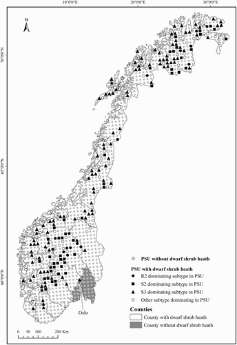
As members of the team responsible for implementing AR18X18, we had access to unpublished results that show dwarf shrub heath is the most common vegetation type in the low alpine region in Norway. It can also be found in open or deforested areas below the forest line. Based on the results we accessed from AR18X18, the estimated coverage of dwarf shrub heath is c.12% of the total Norwegian mainland and 24.7% of the mountain areas. Dwarf shrub heath is found in 15 of the 19 counties in Norway (Fig. 1).

Fig. 1. Distribution of the AR18X18 grid throughout Norway; the dominating vegetation type is decided by the highest number of Secondary Statistical Unit (SSU) points in each Primary Statistical Unit (PSU); R2: Betula nana – Empetrum nigrum coll. subtype. S2: Juniperus communis – Betula nana heath; S3: Vaccinium myrtillus – Phyllodoce caerulea heath and Empetrum nigrum coll. heath

A mixture of nine different vegetation subtypes was found inside dwarf shrub heath polygons. Three of the subtypes were subtypes of dwarf shrub heath vegetation. These made up 69.3% of the observations at the SSU points. The six subtypes that represented other vegetation subtypes made up the remaining 30.7% of the observations. The most frequent subtype in dwarf shrub heath was Vaccinium myrtillus – Phyllodoce caerulea heath and Empetrum nigrum coll. heath (S3), found on 39.7% of the SSU points. The second and third most frequent subtype was Juniperus communis – Betula nana heath (S2) and Betula nana – Empetrum nigrum coll. subtype (R2), respectively found on 20.4% and 9.2% of the SSU points. The representation of the other subtypes inside dwarf shrub heath polygons is listed in Table 1.

The results of the ANOVA test carried out first with all nine subtypes and subsequently with only the three subtypes R2, S2 and S3 are shown in the columns headed ‘F-values’ and ‘p-values’ in Table 2. The difference between the subtypes was significant (p < 0.05) for the mean values of both environmental gradients in both cases (Table 2).

Table 2. The F-values and the P-values from the one-way ANOVA test (8 and 441 df) for Sections and Zones, and the coefficient values from the first linear discriminant

Environmental variable	F-value	P-value	LD1*
All subtypes
Sections	13.4120	0.0000	0.5810
Zones	6.0976	0.0000	0.1500
Defined subtypes (R2, S2 and S3)
Sections	30.9160	0.0000	-0.4985
Zones	14.0980	0.0000	0.1139

Note: * Linear discriminant 1

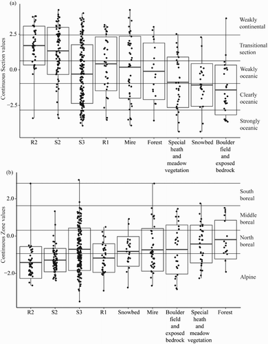
LDA, was carried out with the gradient variables, first using all nine subtypes and thereafter using only the three subtypes defined as dwarf shrub heath. The scores of the gradients (shown in column LD1 in Table 2) indicate that the oceanic–continental gradient represented as Sections is the most important for separating the subtypes inside dwarf shrub heath.

The box plot of section values for the subtypes shows that S2 and R2 have mean values situated in the transitional section of the oceanic–continental gradient, and standard deviation reaching up to the weakly continental section (Figure 2a). The boulder field and exposed bedrock and snowbed subtypes have mean values in the clearly oceanic section of this gradient, while the remaining subtypes have means in the weakly oceanic section. The pairwise t-test along this gradient shows a significant difference (p < 0.01) between S2 and R2 on one hand, and S3, special heath and meadow vegetation, snowbed and boulder field and exposed bedrock on the other hand (Appendix 2a). With respect to the zonal gradient, dwarf shrub heath is mainly found in the part of the gradient characterized as alpine and north boreal zones, as expected for a mountainous vegetation type. The mean zonal value of R2, S2 and R1 is in the alpine zone, while the other subtypes have a mean zonal value in the north boreal zone (Figure 2b). S3 has a distribution reaching across all of the zones. The results of the pairwise t-test showed a significant difference between sites, with R2 and S2 and sites with the subtypes S3, special heath and meadow vegetation and forest (Appendix 2b).

Fig. 2. Box plot with mean and ± SD of the distribution of the different subtypes in dwarf shrub heath according to the environmental gradients; a) Sections; b) Zones (representing principal components PC1 and PC2 in Bakkestuen et al. 2008); R1: Loiseleuria procumbens – lichen/bryophyte subtype; R2: Betula nana – Empetrum nigrum coll. subtype. S2: Juniperus communis – Betula nana heath; S3: Vaccinium myrtillus – Phyllodoce caerulea heath and Empetrum nigrum coll. heath

Discussion

One objective of our study was to examine the variation in areas classified as dwarf shrub heath. The results revealed two different kinds of variation. The first kind is variation in terms of subtypes of the botanical vegetation type dwarf shrub heath. The second kind is variation in terms of other vegetation subtypes appearing inside the polygons classified as dwarf shrub heath on the map (see Fig. 1). The discussion will be organized accordingly. In the following, we first discuss the composition of the dwarf shrub heath in terms of subtypes of this vegetation type. Thereafter, we discuss the variation within the map units classified as dwarf shrub heath, including the variation caused by inclusion of other vegetation subtypes. Finally, we discuss how these findings can be used in the development of vegetation surveys and mapping systems.

Subtypes of dwarf shrub heath

The botanical vegetation type dwarf shrub heath is composed of three subtypes – R2, S2 and S3 (Fremstad 1997; Rekdal & Larsson 2005) – and the variation showed strongest coherence with the oceanic–continental gradient. This gradient is thought to be a key determinant for vegetation composition in Norway (Moen 1998; Bakkestuen et al. 2008). One exception is alpine tundra vegetation in Northern Norway, where microclimatic conditions are the most important factor (Löffler & Pape 2008). R2 and S2 were typically transitional and continental subtypes. S3 had a wide geographical distribution, but tended to favour oceanic locations. Along the zonal gradient, R2 and S2 were the most alpine subtypes, whereas S3 was found in more boreal locations. The combination of the two gradients showed R2 as slightly more continental and alpine than S2. R2 typically made up the more barren locations in the alpine zone within dwarf shrub heath.

The descriptions of the subtypes in the Fremstad classification system are expert assessments reflecting regional climatic variants (Fremstad 1997). The findings from our study support the expert judgments reflected in the definition of the subtypes.

The inclusion of six additional, alien vegetation subtypes inside dwarf shrub heath polygons was an effect of the cartographic generalization involved in vegetation mapping, which we discuss in further detail below. This variation can also be interpreted in terms of landscape appearance. It shows the type landscape of which dwarf shrub heath forms a part. The subtype R1, as an example, is present in and around dwarf shrub heath in the alpine and north boreal areas. The subtype showed some coherence with R2 and S2, but was less distinctly divided from S3.

The remaining landscape subtypes – mire, forest, special heath and meadow vegetation, snowbed, and boulder field and exposed bedrock – showed stronger coherence with S3 than with R2 and S2. Mean values were located in the weakly or clearly oceanic areas and in the north boreal zone. In general, the oceanic regions showed a greater diversity of subtypes inside dwarf shrub heath. This was probably due to more fragmentation of the ‘Sections’ and ‘Zones’ along the coastal areas of Norway.

The subtypes special heath and meadow vegetation and mire, demonstrate the existence of patches influenced by small-scale topographic differences, microclimatic conditions, special soil conditions or culturally influenced areas (i.e. grazing land) in the typical dwarf shrub heath. These groups are composed of very different vegetation types. Mire showed a broad distribution regarding both Sections and Zones and was found from the oceanic to the continental regions, as well as from boreal to alpine sites. Special heath and meadow vegetation was more common in the oceanic areas, but with outliers in other regions.

The subtype snowbed inside dwarf shrub heath is mainly observed in the oceanic areas, especially in the north boreal and alpine oceanic regions, which are known to be the main regions for snowbeds in Norway (Fremstad 1997). As expected, the subtype forest was most frequent in north and middle boreal areas.

Boulder field and exposed bedrock are occasionally found inside dwarf shrub heath in the oceanic areas, particularly in the north boreal and alpine zone. Typical locations are exposed coastal areas and the transitional section between the low alpine and middle alpine areas, where the vegetation cover becomes more scattered.

The results of the analysis indicated that the gradients are influential with respect to the distribution of subtypes of dwarf shrub heath, but they do not provide sufficient information to enable separation of the majority of the subtypes based on the environmental gradients alone. We therefore hypothesize that local variation in terms of, for example, microclimate, topography and micro-scale geology, are also significant. However, the available data did not allow for further investigation of this assertion.

Map generalization of dwarf shrub heath

The variations recognized as intra-class variation and landscape variation can be interpreted and explained using elements from geographic information science (GIS). One such explanation is linked to the classification process. Classification is a conceptual simplification whereby rich and complex vegetation is characterized using a nomenclature consisting of a limited set of classes (Mucina 1997; Peet & Roberts 2012). A second explanation is linked to the geometrical simplification known as map generalization, whereby fuzzy boundaries are drawn as simplified lines on a map (Painho 1995; Weibel & Dutton 1999). The result of these two processes is a combination of conceptual and geometrical simplification that leads to unrecognized variation within the sampling classes.

An additional cartographic concept concerned with readability is relevant here. Even when it is possible to draw a crisp border between vegetation types, the border may be too complex for the map. It is therefore necessary to simplify the polygons when narrow vegetation corridors are present or the distribution of the vegetation types constitutes patterns that are too complex for map visualization (Shea & McMaster 1989). It is also impossible to capture observations with small acreage (small-scale variation in nature), due to the chosen minimum mapping unit size (Stohlgren et al. 1997).

Uncertainty in vegetation classification

In addition to classification and generalization, misclassification of vegetation types and spatial displacement of boundaries can affect the accuracy of a vegetation map (Cherrill & McClean 1995). Large surveys such as AR18X18 are carried out by field crews. Considerable effort is made to harmonize the crew members’ perceptions of the vegetation types, but different understandings of the classification scheme can exist with respect to the fuzzy transitions between classes and for areas without a distinct plant composition.

Misclassification is a major concern when classifying vegetation (e.g. Cherrill & McClean 1999a; 1999b; Hearn et al. 2011). Therefore, only highly experienced personnel were used as field crew in the initial phase of AR18X18. The vegetation types in the VK50 system can also be considered as relatively distinct (Rekdal & Larsson 2005). The number of class identification errors concerning the interpretation of the SSU points, using the more detailed vegetation mapping system developed by Fremstad (1997), is probably more frequent than identification errors linked to the VK50 classes, since the interpretation of the more detailed Fremstad classification system requires more botanical knowledge. The system also has a relatively large number of subtypes, many with similar species compositions, which makes misidentification more common. Further research is needed to identify the extent of identification errors linked to the use of the two mapping systems.

Location error of the PSUs is considered negligible because several sources (i.e. GPS, orthophotos and topographic maps) were used to secure the correct locations. However, location error of the SSUs could occur due to poor use or inaccuracy of the handheld GPS.

Further perspectives

Our study demonstrated the feasibility of combining a fairly simple and cost-effective point sampling survey with a broader wall-to-wall vegetation survey. Although demonstrated with data from a national sampling survey, the method is equally applicable in a complete wall-to-wall survey of any area where variation in the mapping classes is expected. Relevant examples could be a national park or an administrative area.

Wall-to-wall mapping surveys are expensive, and the expenses increase as the classification system becomes more detailed. From our professional experience, the cost per area unit for wall-to-wall mapping using the detailed Fremstad system is around five times as high as the cost of using the less detailed VK50 system. Furthermore, detailed classification systems are more demanding with respect to harmonization of the field crew (Strand 1996; Strand et al. 2002). The hybrid approach using a simple but sufficient classification system for the wall-to-wall survey and strengthening the survey with a point sample of more detailed observations is a feasible compromise. In this article, we have demonstrated that this combination is workable, such that the point survey can significantly increase the knowledge available from a wall-to-wall survey and also provide useful summaries of the errors involved.

An example of when the combined approach could be used is the new classification system recently introduced for use in the environmental sector in Norway: Natur i Norge (NiN) (Halvorsen 2011; Halvorsen et al. 2015). NiN is a hierarchical system with several levels of detail. It is currently used for wall-to-wall mapping of small protected areas. A cost-efficient use for large areas (e.g. national parks) could involve a less detailed level of the system for wall-to-wall mapping and a more detailed level for an accompanying point survey in the study area. However, it is important that the point sampling is carried out as a survey with known statistical properties and valid randomization.

In our study, we set out to examine the areas mapped as dwarf shrub heath in the national survey of land cover and outfield land resources. The population was thus defined as areas assigned to this particular vegetation class and enabled us to document two kinds of variation: the intra-class variation of the vegetation class, and the landscape variation attributed to cartographic generalization. A different useful approach would be to examine all of the sample points from the survey, including those located in map units classified as vegetation types other than dwarf shrub heath. Such an approach could provide information about the possible statistical bias in the area estimate based on the wall-to-wall survey. More importantly, the approach describes the composition of the entire population (as opposed to the individual mapping classes) with respect to the detailed classes. The difference between the two methods is that, in our study, the selection of the sample points used described the variation among the mapping units classified as dwarf shrub heath. Using all sample points throughout the entire region that has been mapped would provide a more complete description of the composition of the vegetation.

The sampling strategy adopted for AR18X18 was a constraint in our study. Only 10 SSU points were available inside each PSU. An even more limited number of SSU points was available when just one of the VK50 vegetation types was examined. Nevertheless, our approach still turned out to be an applicable and cost-effective way of giving a more detailed description of dwarf shrub heath in Norway. Moreover, combining the data with environmental gradients known to influence the vegetation distribution contributed to a better understanding of the vegetation type. However, having a dataset with a much larger number of SSU points inside the PSU and possibly classified according to a more detailed nomenclature than Fremstad (1997), would have provided better options for analysing the distribution of dwarf shrub heath, or other vegetation types. A methodological study could be conducted to identify the optimal approach to survey data collection and examination of intra-class variation in vegetation types using real world data. Different sample sizes and sampling strategies should be tested, taking into account spatial autocorrelation, in order to provide a basis for analysis of how the description of, for example, dwarf shrub heath, varies with the different designs. More SSU points inside each vegetation type would have allowed for a more complex analysis of the dataset with respect to how the vegetation types correlated with the environmental variables. An approach could be to perform a mixed multinomial modelling procedure, or to analyse such a dataset by performing a canonical correlation analysis (ter Braak & Smilauer 2002), provided that the number of sample points inside each PSU is large enough to characterize the amount of each class as a continuous variable.

Conclusions

Dwarf shrub heath in Norway is a broad vegetation type composed of a number of subtypes. Our study has shown that the variation in dwarf shrub heath is linked to environmental gradients. It was possible to use existing area frame survey data when examining intra-class variation in this vegetation types. The method was cost-effective and gave a good description of the vegetation type, but with some limitations. The study revealed two different dimensions of variation. The first dimension was the expected intra-class variation in terms of a regional variation in dwarf shrub heath subtypes. The second dimension was the inclusion of other vegetation subtypes inside dwarf shrub heath polygons, showing how dwarf shrub heath is intermixed with several vegetation types within the landscape. The latter dimension was linked to the classification system and the map generalization process. Both kinds of variation were associated with explanatory environmental gradients, and the oceanic-continental gradient was seen as the most important factor in the distribution of the defined subtypes.

Acknowledgements

We are particularly grateful to Per K. Bjørklund, Anders Bryn, and two anonymous reviewers for providing valuable comments on an earlier draft of this article and to Gregory Taff for linguistic corrections to an earlier version of the manuscript. The study on which this article is based was fundeded by the Norwegian Institute of Bioeconomy Research (NIBIO).

Appendix 1. Common species found in dwarf shrub heath defined by the VK50 system for vegetation mapping at intermediate scale (1:20,000 – 1:50,000) (Rekdal & Larsson 2005); species common in areas with high precipitation are marked with *

Character and lead species	Other common species
Betula nana	Anthoxanthum odoratum (L.)
Vaccinium myrtillus	Solidago virgaurea
Empetrum nigrum	Pedicularis lapponica
Avenella flexuosa	Pleurozium schreberi
Cornus suecica*	Cladonia ssp.
Hylocomium splendens	Juniperus communis
Cladonia stellaris	Salix glauca var glauca
	Salix lapponum
	Calluna vulgaris
	Vaccinium vitis-idaea
	Vaccinium uliginosum
	Phyllodoce caerulea
	Nardus stricta*
	Melampyrum pratense
	Lysimachia europaea
	Cetraria islandica
	Stereocaulon paschale (L.)

Appendix 2. Results (p-values) from the pairwise t-test for the different environmental variables; P-values < 0.01 are marked with grey shading; R1: Loiseleuria procumbens – lichen/bryophyte subtype; R2: Betula nana – Empetrum nigrum coll. subtype; S2: Juniperus communis – Betula nana heath; S3: Vaccinium myrtillus – Phyllodoce caerulea heath and Empetrum nigrum coll. heath.

(a) Sections	Mire	R1	R2	S2	S3	Forest	Snowbed	Special heath and meadow vegetation
R1	1	-	-	-	-	-	-	-
R2	0.0068	0.1034	-	-	-	-	-	-
S2	0.057	0.7014	1	-	-	-	-	-
S3	1	1	3.20E-08	5.00E-08	-	-	-	-
Forest	1	1	0.0285	0.1653	1	-	-	-
Snowbed	0.3793	0.1238	6.10E-07	4.70E-06	1	1	-	-
Special heath and meadow vegetation	0.5918	0.1844	2.20E-07	1.50E-06	1	1	1	-
Boulder field and exposed bedrock	0.0219	0.0059	1.20E-09	6.70E-09	0.1628	0.8791	1	1
(b) Zones	Mire	R1	R2	S2	S3	Forest	Snowbed	Special heath and meadow vegetation
R1	1	-	-	-	-	-	-	-
R2	0.06637	1	-	-	-	-	-	-
S2	0.1615	1	1	-	-	-	-	-
S3	1	0.47872	0.00153	0.00155	-	-	-	-
Forest	1	0.03398	0.0008	0.00184	1	-	-	-
Snowbed	1	1	0.77837	1	1	1	-	-
Special heath and meadow vegetation	1	0.08542	0.00092	0.00187	1	1	1	-
Boulder field and exposed bedrock	1	1	0.16905	0.41541	1	1	1	1

References

- Aune-Lundberg, L. & Strand, G.-H. 2014. Comparison of variance estimation methods for use with two-dimensional systematic sampling of land use/land cover data. Environmental Modelling & Software 61, 87–97.
- Bakkestuen, V., Erikstad, L. & Halvorsen, R. 2008. Step-less models for regional environmental variation in Norway. Journal of Biogeography 35, 1906–1922. doi: 10.1111/j.1365-2699.2008.01941.x
- Box, E.O. 1981. Macroclimate and Plant Forms: An Introduction to Predictive Modeling in Phytogeography. The Hauge: Dr W. Junk.
- Box, E.O. & Fujiwara, K. 2005. Vegetation types and their broad-scale distribution. Van Der Maarel, E. & Franklin, J. (eds.) Vegetation Ecology, 455–485. 2nd ed. Oxford: John Wiley & Sons.
- Bryn, A., Dourojeanni, P., Hemsing, L.Ø. & O’Donnell, S. 2013. A high-resolution GIS null model of potential forest expansion following land use changes in Norway. Scandinavian Journal of Forest Research 28, 81–98. doi: 10.1080/02827581.2012.689005
- Cherrill, A. & McClean, C. 1995. An investigation of uncertainty in field habitat mapping and the implications for detecting land cover change. Landscape Ecology 10, 5–21. doi: 10.1007/BF00158550
- Cherrill, A. & McClean, C. 1999a. The reliability of ‘Phase 1’ habitat mapping in the UK: The extent and types of observer bias. Landscape and Urban Planning 45, 131–143. doi: 10.1016/S0169-2046(99)00027-4
- Cherrill, A. & McClean, C. 1999b. Between-observer variation in the application of a standard method of habitat mapping by environmental consultants in the UK. Journal of Applied Ecology 36, 989–1008. doi: 10.1046/j.1365-2664.1999.00458.x
- Conrad, V. 1946. Usual formulas of continentality and their limits of validity. Eos, Transactions American Geophysical Union 27, 663–664. doi: 10.1029/TR027i005p00663
- Couclelis, H. 1992. People manipulate objects (but cultivate fields): Beyond the raster vector debate in GIS. Frank, A.U. & Campari, I. (eds.) Theories and Methods of Spatio-temporal Reasoning in Geographic Space: Lecture Notes in Computer Science, 65–77. Berlin: Springer-Verlag.
- De Frenne, P., Graae, B.J., Rodríguez-Sánchez, F., Kolb, A., Chabrerie, O., Decocq, G., De Kort, H., De Schrijver, A., Diekmann, M., Eriksson, O., Gruwez, R., Hermy, M., Lenoir, J., Plue, J., Coomes, D.A. & Verheyen, K. 2013. Latitudinal gradients as natural laboratories to infer species’ responses to temperature. Journal of Ecology 101, 784–795. doi: 10.1111/1365-2745.12074
- Dramstad, W.E., Fjellstad, W.J., Strand, G.-H., Mathiesen, H.F., Engan, G. & Stokland, J.N. 2002. Development and implementation of the Norwegian monitoring programme for agricultural landscapes. Journal of Environmental Management 64, 49–63. doi: 10.1006/jema.2001.0503
- Ferrier, S. 2002. Mapping spatial pattern in biodiversity for regional conservation planning: Where to from here? Systematic Biology 51, 331–363. doi: 10.1080/10635150252899806
- Fremstad, E. 1997. Vegetasjonstyper i Norge. NINA Temahefte 12. Trondheim: Norsk Institutt for Naturforskning.
- Goodchild, M.F. 2011. Scale in GIS: An overview. Geomorphology 130, 5–9. doi: 10.1016/j.geomorph.2010.10.004
- Halvorsen, R. 2011. Faglig grunnlag for naturtypeovervåkning i Norge – begreper, prinsipper og verktøy. Naturhistorisk museum Rapport 10. Oslo: Naturhistorisk museum, Universitetet i Oslo.
- Halvorsen, R., Bryn, A., Erikstad, L. & Lindgaard, A. 2015. Natur i Norge – NiN: Versjon 2.0.0. Trondheim: Artsdatabanken.
- Hearn, S.M., Healey, J.R., McDonald, M.A., Turner, A.J., Wong, J.L.G. & Stewart, G.B. 2011. The repeatability of vegetation classification and mapping. Journal of Environmental Management 92, 1174–1184. doi: 10.1016/j.jenvman.2010.11.021
- Ihse, M. 2007. Colour infrared aerial photography as a tool for vegetation mapping and change detection in environmental studies of Nordic ecosystems: A review. Norsk Geografisk Tidsskrift–Norwegian Journal of Geography 61, 170–191. doi: 10.1080/00291950701709317
- Keeler-Wolf, T. 2007. The history of vegetation classification and mapping in California. Keeler-Wolf, T., Barbour, M.G. & Schoenherr, A.A. (eds.) Terrestrial Vegetation of California, 1–42. 3rd ed. Berkley: University of California Press.
- Kent, M. 2012. Vegetation Description and Data Analysis: A Practical Approach. Oxford: John Wiley & Sons.
- Kent, M. & Coker, P. 1992. Vegetation Description and Analysis: A Practical Approach. Chichester: John Wiley & Sons.
- Küchler, A.W. & Zonneveld, I.S. 1988. Vegetation Mapping. Dordrecht: Springer.
- Löffler, J. & Pape, R. 2008. Diversity patterns in relation to the environment in alpine tundra ecosystems of Northern Norway. Arctic, Antarctic, and Alpine Research 40, 373–381. doi: 10.1657/1523-0430(06-097)[LOEFFLER]2.0.CO;2
- McGarvey, R., Burch, P. & Matthews, J.M. 2015. Precision of systematic and random sampling in clustered populations: Habitat patches and aggregating organisms. Ecological Applications 26, 233–248. doi: 10.1890/14-1973
- McLachlan, G.J. 2004. Discriminant Analysis and Statistical Pattern Recognition. Hoboken: John Wiley & Sons.
- Moen, A. 1998. Nasjonalatlas for Norge: Vegetasjon. Hønefoss: Statens kartverk.
- Morrison, D.G. 1969. On the interpretation of discriminant analysis. Journal of Marketing Research 6, 156–163. doi: 10.2307/3149666
- Mucina, L. 1997. Classification of vegetation: Past, present and future. Journal of Vegetation Science 8, 751–760. doi: 10.2307/3237019
- Nilsen, L.S. & Moen, A. 2009. Coastal heath vegetation in central Norway. Nordic Journal of Botany 27, 523–538. doi: 10.1111/j.1756-1051.2009.00240.x
- Ørka, H.O., Dalponte, M., Gobakken, T., Næsset, E. & Ene, L.T. 2013. Characterizing forest species composition using multiple remote sensing data sources and inventory approaches. Scandinavian Journal of Forest Research 28, 677–688. doi: 10.1080/02827581.2013.793386
- Painho, M. 1995. The effects of generalization on attribute accuracy in natural resource maps: GIS and generalization. Muller, J.C., Lagrange, J.P. & Weibel, R. (eds.) Methodology and Practice, 194–206. London: Taylor & Francis.
- Peet, R.K. & Roberts, D.W. 2012. Classification of natural and semi-natural vegetation. Van Der Maarel, E. & Franklin, J. (eds.) Vegetation Ecology, 28–70. New York: John Wiley & Sons.
- Rekdal, Y. & Larsson, J.Y. 2005. Veiledning i Vegetasjonskartlegging – M 1:20 000–50 000. NIJOS rapport 05. Ås: Norsk Institutt for Jord og Skogkartlegging.
- Shea, K.S. & McMaster, R.B. 1989. Cartographic generalization in a digital environment: When and how to generalize. American Society for Photogrammetry and Remote Sensing (eds.) Auto-Carto 9: Ninth International Symposium on Computer-Assisted Cartography, Baltimore, Maryland, April 2–7, 56–67. Falls Church, VA: American Society for Photogrammetry and Remote Sensing & American Congress on Surveying and Mapping. ISBN-10: 0944426557
- Ståhl, G., Allard, A., Esseen, P.-A., Glimskär, A., Ringvall, A., Svensson, J., Sundquist, S., Christensen, P., Torell, Å., Högström, M., Lagerqvist, K., Marklund, L., Nilsson, B. & Inghe, O. 2011. National inventory of landscapes in Sweden (NILS)—scope, design, and experiences from establishing a multiscale biodiversity monitoring system. Environmental Monitoring and Assessment 173, 579–595. doi: 10.1007/s10661-010-1406-7
- Stohlgren, T.J., Chong, G.W., Kalkhan, M.A. & Schell, L.D. 1997. Multiscale sampling of plant diversity: Effects of minimum mapping unit size. Ecological Applications 7, 1064–1074. doi: 10.1890/1051-0761(1997)007[1064:MSOPDE]2.0.CO;2
- Strand, G.-H. 1996. Detection of observer bias in ongoing forest health monitoring programmes. Canadian Journal of Forest Research 26, 1692–1696. doi: 10.1139/x26-191
- Strand, G.-H. 2013. The Norwegian area frame survey of land cover and outfield land resources. Norsk Geografisk Tidsskrift–Norwegian Journal of Geography 67, 24–35. doi: 10.1080/00291951.2012.760001
- Strand, G.-H., Dramstad, W. & Engan, G. 2002. The effect of field experience on the accuracy of identifying land cover types in aerial photographs. International Journal of Applied Earth Observation and Geoinformation 4, 137–146. doi: 10.1016/S0303-2434(02)00011-9
- ter Braak, C.J.F. & Smilauer, P. 2002. CANOCO Reference Manual and CanoDraw for Windows User’s Guide: Software for Canonical Community Ordination (Version 4.5). Wageningen: Biometris.
- Thackway, R., Lee, A., Donohue, R., Keenan, R.J. & Wood, M. 2007. Vegetation information for improved natural resource management in Australia. Landscape and Urban Planning 79, 127–136. doi: 10.1016/j.landurbplan.2006.02.003
- Weibel, R. & Dutton, G. 1999. Generalising spatial data and dealing with multiple representations. Geographical Information Systems 1, 125–155.
- Werger, M.J.A. & Sprangers, J.T.C. 1982. Comparison of floristic and structural classification of vegetation. Vegetatio 50, 175–183. doi: 10.1007/BF00364111
- Westhoff, V. & Van Der Maarel, E. 1978. The Braun-Blanquet approach. Whittaker, R.H. (ed.) Classification of Plant Communities, 287–399. The Hague: Junk.
- Whittaker, R. & Beard, J. 1978. The physiognomic approach. Whittaker, R.H. (ed.) Classification of Plant Communities, 33–64. Dordrecht: Springer.
- Yu, Q., Gong, P., Clinton, N., Biging, G., Kelly, M. & Schirokauer, D. 2006. Object-based detailed vegetation classification with airborne high spatial resolution remote sensing imagery Photogrammetric Engineering & Remote Sensing 13, 799–811. doi: 10.14358/PERS.72.7.799