Seeking commonalities of community resilience to natural hazards: A cluster analysis approach

ABSTRACT

The aim of the study on which the article is based was to identify groups of communities with similar resilience profiles, using Norwegian municipalities as a case. The authors used a set of socioeconomic and environmental indicators as measures of municipalities’ resilience and performed a cluster analysis to divide the municipalities into groups with similar multivariate resilience signatures. The results revealed six groups of municipalities that, apart from their unique combinations of indicator scores, featured certain spatial patterns, such as an “urban cluster” with urbanized municipalities and a “suburban cluster” with municipalities concentrated around major cities. The authors conclude that municipalities in each of the groups shared aspects that made them either more or less resilient to natural hazards, which could make them potential targets for shared interventions. Additionally, the authors conclude that clustering can be used to identify municipalities with similar resilience features and that could benefit from networking and sharing operational planning as a way to improve their respective communities' resilience to natural hazards.

KEYWORDS:

• cluster analysis
• community capacities
• indicators
• Norway
• resilience measurement

Introduction

Recent quantitative research on vulnerability (Cutter et al. 2003; Holand et al. 2011) and resilience to natural hazards (Cutter et al. 2014; Yoon et al. 2016) has focused on identifying places or communities either most at risk or most resilient to the adverse effects of hazardous events. In most cases, researchers have first compiled a set of indicators based on a theoretical framework and then merged the indicators into a composite index (Cutter et al. 2000; Rød et al. 2015). Thereafter, the resulting index scores have been ranked from least to most vulnerable or resilient and depicted on a map to facilitate visual examination of their geographies.

In this article, we depart from the indexation approach. Instead, we draw upon the pattern analysis in geography research in which various approaches have been used, such as fuzzy classification (Cullum et al. 2017), dynamic patterns (Petschel-Held et al. 1999) and cluster analysis (e.g., Sietz et al. 2011). We employed the latter approach in an attempt to identify commonalities of community resilience to natural hazards. The cluster analysis approach enabled us to divide Norwegian municipalities into groups by exploiting similarities regarding their indicators of resilience to natural hazards. Hence, we were able to discover typical multivariate resilience signatures of the municipalities, namely the patterns embedded in the multidimensional space of the indicators. Rather than forcing the indicators into an abstract index that created distinct resilience scores for each municipality, we reduced data dimensionality and grouped Norwegian municipalities that shared similar resilience profiles into clusters.

From a policy perspective, as considered in earlier research, for example on socio-ecological patterns of farming systems’ vulnerabilities in the African drylands (Sietz et al. 2017), typical multivariate resilience signatures mean that if a group of municipalities exhibits similar challenges regarding certain resilience indicators, such municipalities can potentially benefit from cooperation in designing common interventions and mitigation strategies, rather than executing interventions and adaptation actions independently and individually. Further, such cooperation may result in more effective adaptation efforts and be of value to all who are responsible for mitigation actions.

By employing k-means++ clustering, we identified groups with distinct multivariate resilience signatures and spatial patterns within Norwegian municipalities. We used these groups to address the following research questions:

RQ1: How do the municipalities from various groups differ with regard to their community resilience indicators?

RQ2: What are the spatial patterns of the municipalities that constitute specific groups? Do the groups of municipalities constitute spatially consistent regions or are the municipalities of one cluster scattered throughout Norway?

Background

Community resilience to natural hazards

There is not one precise definition of community resilience. In finding some consensus in the literature, Cutter et al. (2014, 65) propose the following:

Disaster resilience enhances the ability of a community to prepare and plan for, absorb, and recover from, and more successfully adapt to actual or potential adverse events in a timely and efficient manner including the restoration and improvement of basic functions and structures.

This definition is broad enough to be applicable to different hazards and different sectors of society, as well as to different interpretations of what constitutes community.

Given the definitional ambiguity relating to ‘community resilience’, it is not surprising that conceptual frameworks for community resilience are manifold. One of the most influential frameworks was developed by Norris et al. (2008), who see community resilience as a set of networked capacities. Others apply a capitals approach to community resilience, focusing on social capital (Ritchie & Gill 2006; Aldrich 2012; Aldrich & Meyer 2015), community capital (Miles & Chang 2011), or a combination of capitals (Mayunga 2007; Peacock 2010). Also, some authors consider community resilience part of a system, such as the economy (Rose 2004; 2007; Rose & Krausmann 2013) or governance (Tierney 2012) or they link resilience to place-based attributes of the community (Cutter et al. 2008; Frazier et al. 2014). It is evident from the plurality of definitions and conceptual models that community resilience is inherently difficult to measure, as there is no agreement on which model should be used, which characteristics should be included, or which reference group, location, or system should be chosen. Nonetheless, there is increasing interest in measuring community disaster resilience. The growing number of natural hazard threats due to climate change calls for better knowledge not only about exposed and vulnerable locations but also about the resilience capabilities of local communities and their spatial distribution.

Assessment of community resilience

There is no uniform approach to the assessment of community resilience, since implemented assessment strategies depend on the objectives, motivations, and interpretations of the community resilience concept of those who do the assessment. Assessment strategies will differ according to whether resilience is understood as a process, an outcome, or both, whether it is applied to a single community or a larger geographic region, and whether it focuses on one resilience dimension or multiple resilience dimensions. The approaches used thus far fall roughly into three categories: indices, scorecards, and tools (for a systematic discussion of resilience assessment approaches used in the USA, see Cutter 2016).

An index combines a set of indicators into a single metric. Index construction is usually a top-down approach, based on existing quantitative data. When striving for comparability across space or time, indexation is the measurement method of choice. As a result, the number of resilience indices is growing steadily (various resilience indices have been proposed by, e.g., Cutter et al. 2010; 2014; Peacock 2010; Sherrieb et al. 2010; Miles & Chang 2011; Frazier et al. 2014; Burton 2015; Cox & Hamlen 2015; Yoon et al. 2016). However, as argued by Cai et al. (2018), quantitative community resilience measurement approaches typically lack empirical validation and inferential ability. Moreover, they do not reveal concrete adaptation strategies.

Scorecards are used to assess the progress made towards a particular goal by asking questions about the presence or absence of certain attributes and recording them on a scale (e.g. from 1 to 10, from very poor to excellent). A final score can be calculated based on the provided answers. Scorecards are based on qualitative data inputs and are usually intended for localized self-assessments in communities (for an example of a scorecard, see Sempier et al. 2010).

Tools provide ready-made mechanisms for either community self-assessments or the construction of an index, with sample procedures, survey guidelines and/or data inputs. Such mechanisms have been proposed by Pfefferbaum et al. (2013), Twigg (2009), and the UNDP (2014).

The above-described assessment approaches provide either detailed information about the resilience capabilities of local communities (scorecard self-assessments) or single metrics intended to capture overall resilience or resilience dimensions (indices and subindices). Both types of results can be useful for mitigation planning and adaptation planning at different scales—the former at a local scale and the latter allowing for easy comparisons among communities at regional or national scales. However, the results of indexation exercises can be hard to interpret or use in practice, as it is often unclear how the index has been constructed and how certain indicators contribute to the construct. Therefore, decision-makers and practitioners may not understand the resulting indices because they will be too abstract (Bohman et al. 2014). Some authors even warn that indices should not be used to inform policymaking (Barnett et al. 2008).

Cluster analysis offers a compromise and allows us to gain a systematic understanding of resilience at an intermediate level of complexity, between an all-embracing perspective (i.e. the composite indicator approach) and the particularities of individual cases (Sietz et al. 2017). To avoid the reductionist nature of indexation results, yet still allow for comparability between communities, we propose a different approach to community resilience assessment. Rather than seeking to identify the most or least resilient communities, we aim to identify clusters of municipalities—ideally, geographically consistent ones—with similar multivariate signatures in terms of community resilience. Although we focused on Norwegian municipalities in our study, other administrative divisions than municipalities can be used, if their multivariate characteristics are available.

The clusters of municipalities, which have similar multivariate signatures, correspond to what Sietz et al. (2017) call archetypes and consist of “peer” communities that can benefit from the sharing of knowledge and experiences. If certain municipalities feature shortcomings regarding specific resilience indicators, then interventions and mitigation strategies may be executed for the whole group, rather than for individual municipalities. To identify these groups with similar resilience signatures, our approach employs cluster analysis. The method ensures that, on the one hand, the groups consist of municipalities that are as similar as possible according to their resilience indicator values, but, on the other hand, the groups are as different as possible from other groups.

Cluster analysis and its use for geographic data

As a method, clustering groups the most similar multivariate data entities into classes. Since clustering helps to reveal underlying structures in multivariate geographic data it is applied for different purposes in various geographic subdisciplines. For instance, in physical geography, it has been used to differentiate regions based on their climate parameters such as daily precipitation and temperature (Leuprecht & Gobiet 2010) or to identify regional climate change patterns (Mahlstein & Knutti 2010). By contrast, in social and economic geography clustering serves as a valuable tool to, for example, detect crime hot spots (Grubesic & Murray 2001), study spatiotemporal patterns of neighborhood socioeconomic change in cities (Delmelle 2016), create homogeneous groupings of geographic areas with regard to similar exposure to the risk of insurance losses (Jennings 2008), and to investigate socio-ecological patterns of farming systems’ vulnerability in African drylands in order to examine the potential for sustainable agricultural intensification (Sietz et al. 2017). Furthermore, as reported by Lam et al. (2016), k-means clustering has been employed with discriminant analysis in the resilience inference measurement (RIM) model in order to derive resilience rankings, thus enabling validation and inference. Mihunov et al. (2018) used RIM to identify four variables representing the social, economic, agriculture, and health sectors as the main resilience indicators.

Furthermore, clustering can play a valuable role in research on climate change adaptation. Due to global climate change, it is expected that natural hazards will become more frequent and severe, including in the Nordic countries (Rød et al. 2015). In this context, cluster analysis can be used to investigate whether Norwegian municipalities can be grouped according to their similarity across a set of community resilience indicators and whether the resulting groups would have a spatial pattern forming spatially consistent regions. However, as in all clustering exercises, uncertainty exists with regard to the appropriate number of clusters and the justification of the identified clusters. Therefore, in any cluster analysis, emphasis should be placed on the meaningfulness of the cluster selection; clusters should not be arbitrary or artificial (OECD-JRC 2008).

Study data

The set of indicators of community resilience selected for the clustering procedure used in our study was originally compiled by Scherzer et al. (2019), who used it to construct a community resilience index for Norway. Their initial indicator selection was guided by previous studies of vulnerability and community resilience (Cutter et al. 2010; Flanagan et al. 2011; Tate 2012; Cutter et al. 2014; Singh-Peterson et al. 2014; Burton 2015; Cox & Hamlen 2015). More than 100 variables were initially collected for all 428 Norwegian municipalities for the year 2014. Following conceptual considerations and statistical analysis, the number of variables was then reduced to a final set of 47 variables (for a detailed account of the indicator selection process including justifications, see Scherzer et al. 2019). Short definitions and summary statistics relating to the included variables are listed in Table 1.

Table 1. List of variables used in the cluster analysis and their summary statistics

No.	Variable	Short name	Source	Mean	Std. Dev.	Min.	Max.
Social resilience (8 indicators):
1	Percent of the population that is of working age (16–66 years)	WORKING_AGE	SSB	64.64	2.07	58.46	71.62
2	Cars per 1,000 persons	CARS	SSB	524.74	55.53	257.67	719.22
3	Broadband Internet subscriptions per 1,000 persons	INTERNET	SSB	322.82	51.41	114.80	723.63
4	Percent of households that are NOT single-parent households	NOT_SINGLE_PARENT	SSB	94.87	1.09	91.12	98.57
5	Percent of the population that is NOT dependent on social assistance	NOT_ASSISTANCE	SSB	97.47	1.05	90.89	100.00
6	Psychologists per 1,000 persons (mental health)	PSYCHOLOGISTS	SSB	0.35	0.75	0.00	6.77
7	Physicians per 1,000 persons (general health)	DOCTORS	SSB	1.72	2.74	0.00	26.69
8	Gender Equality Index	GENDER_INDEX	SSB	0.67	0.04	0.56	0.79
Economic resilience (7 indicators):
9	Percent of the labor force that is employed	EMPLOYED	SSB	97.51	1.01	92.88	99.55
10	Percent of women in the workforce	FEMALE_EMPLOYED	SSB	76.92	3.67	66.30	88.80
11	Percent of employed persons NOT working in primary industry or tourism	EM_NOT_PRIMARY	SSB	85.60	7.10	46.48	97.68
12	Ratio of large to small businesses (in terms of employees: large >100, small <10)	RATIO_LS_BUSINESSES	SSB	0.01	0.01	0.00	0.11
13	Commercial establishments/enterprises per 1,000 persons	ENTERPRISES	SSB	73.98	18.12	36.37	172.98
14	Lending institutions per 1,000 persons	BANKS	SSB	1.62	1.35	0.00	11.79
15	Turnover per capita retail sales	TURNOVER_RETAIL	SSB	58463.61	28030.63	8027.00	208395.00
Institutional resilience (4 indicators):
16	Net operating expenditure, fire and accident protection per capita	FIRE_ACC_SPEND	SSB	976.57	617.12	307.00	8453.00
17	Net operating surplus as a percentage of gross operating revenues	NET_OP_SURPLUS	SSB	1.24	3.14	-9.00	18.20
18	Mean distance in meters from denser settlement areas to nearest county capital**	DIST_COUNTY_CAP*	Kartverket	61897.20	44563.44	545.54	215380.50
19	Percent of employed persons working in public administration, defense, social security or municipal activities:	EM_MUN_PUBLIC	SSB	29.19	8.63	13.16	86.78
Infrastructure & housing resilience (9 indicators):
20	Fire, police, ambulance stations, and shelters per 1,000 people	RESPONSE	Kartverket	0.35	0.53	0.00	4.74
21	Mean distance in meters from denser settlement areas to the nearest fire or police station**	DIST_FIRE_POLICE*	Kartverket	8992.77	9749.16	1.00	68739.58
22	Mean distance in meters from denser settlement areas to nearest hospital (with emergency services)**	DIST_HOSPITAL*	Kartverket	35281.56	26283.12	1565.50	176593.70
23	Traffic accidents per 1,000 persons	ACCIDENTS*	SSB	1.11	0.80	0.00	6.66
24	Length of major road network in km	ROAD_KM	Kartverket	169.17	98.93	5.68	659.85
25	Length of railway network in km	RAILWAY_KM	Jernbaneverket	9.95	17.78	0.00	101.00
26	Mean distance in meters from denser settlement areas to the nearest airport**	DIST_AIRPORT*	Kartverket	48164.71	33764.10	1368.64	152769.90
27	Percent of employed persons working in public utilities (electricity, water, waste, transportation, communication)	EM_UTILITIES	SSB	7.22	4.95	0.60	43.60
28	Percent of the population living in urban areas	URBAN_POP	SSB	53.34	27.24	0.00	99.14
Community capital (10 indicators):
29	Percent of employed persons working in creative class occupations (i.e., architects, engineers, and scientific researchers)	EM_CREATIVE	SSB	19.89	5.35	7.23	40.34
30	Research & development firms per 1,000 persons	RD_FIRMS	SSB	3.96	2.29	0.00	14.01
31	Places of worship per 1,000 persons	WORSHIP	Kartverket	2.72	1.98	0.19	10.83
32	Museums, libraries, zoos, and botanical gardens per 1,000 persons	MUSEUMS	Kartverket	2.17	2.87	0.00	20.04
33	Sports facilities per 1,000 persons	SPORTS	Kartverket	2.62	2.33	0.00	15.69
34	Parliamentary elections voter turnout (Percent of voting age population)	VOTER_TURNOUT	SSB	76.98	3.75	65.10	91.10
35	Cinemas, youth centers, and clubs per 1,000 persons	CLUBS	SSB	8.63	7.95	0.00	48.39
36	Kindergartens (child care services) per 1,000 persons	CHILD_CARE	SSB	1.39	0.52	0.42	4.74
37	Broadcasters per 1,000 persons (access to information)	BROADCAST	SSB	0.27	0.45	0.00	4.21
38	Absolute in- and out-migration as a percentage of population	MIGRATION*	SSB	10.43	2.96	4.46	20.60
Environmental resilience (9 indicators):
39	Percent land area that is NOT in a flood/storm surge zone	NOT_FLOOD_AREA	NVE	96.36	3.02	79.73	100.00
40	Percent land area that does NOT contain impervious surfaces	NOT_IMPERVIOUS	CORINE	77.06	22.57	9.72	100.00
41	Percent land area that is NOT in landslide zones	NOT_SLIDE_AREA	NVE	95.66	5.86	69.64	100.00
42	Percent of land area that is NOT covered by water bodies (rivers and lakes)	NOT_WATER	Kartverket	94.58	3.53	69.86	99.93
43	Percent land area that serves as natural flood buffer (e.g., wetland, swamp, marsh, mangrove, sand, dune)	NAT_BUFFER	CORINE	18.14	13.79	0.00	60.05
44	Percent land area that is developed open space	DEV_OPENSPACE	CORINE	0.45	1.56	0.00	21.15
45	Percent land area that is arable (cultivated) land	ARABLE_LAND	CORINE	11.59	13.71	0.00	83.27
46	5-year average number of loss-causing extreme weather events (number of NNP payouts for storm, slide, surge, and flood are used as a proxy)	HAZARDS_5YRS*	NNP	32.33	41.87	0.40	403.80
47	Agricultural holdings per 1,000 persons	AG_HOLDINGS	SSB	21.93	18.85	0.00	93.93

Notes: * reverse-scaled variable to match the theoretical orientation of the other variables; ** ln-transformed variable; SSB – Statistics Norway, NVE – Norwegian Water Resources and Energy Directorate, Kartverket – Norwegian Mapping Authority, NNP – Norwegian Natural Perils Pool, CORINE – Coordination of information on the environment, program by the European Commission

Prior to conducting the cluster analysis, we min-max transformed all variables to range from 0 to 1 and reverse-scaled a number of variables to match the theoretical orientation of the other variables.¹ As Scherzer et al.’s study was based on the Baseline Resilience Indicators for Communities (BRIC) developed by Cutter et al. (2014), they adopted the six resilience subdomains described in the original BRIC study (Scherzer et al. 2019). The same variables and subdomains were used in our study. Each municipality thus featured 47 variables divided into the six resilience subdomains: (1) social, (2) economic, (3) institutional, (4) infrastructure & housing, (5) community capital, and (6) environmental.

The social resilience subdomain (1) captures general characteristics of the population that would increase the ability of the population to handle difficult situations or crises. For example, people of working age (WORKING_AGE in Table 1) are generally considered better able to help themselves and others than are children or the elderly. Social resilience is further strengthened by adequate access to physical health care providers (DOCTORS) and mental health care providers (PSYCHOLOGISTS), as well as by good access to transport (CARS) and communication (INTERNET).

The economic resilience subdomain (2) portrays the health and vitality of the local economy. Indicators that represent the general economic vitality of the community include the overall employment rate (EMPLOYED) and the per capita retail turnover (TURNOVER_RETAIL). One key aspect of a functioning economy in any setting is access to financial resources (BANKS). In a crisis, large enterprises are often better able to absorb shocks and to bring in resources from outside the community through business networks (RATIO_LS_BUSINESSES). However, the primary sector and the tourism industry (EM_NOT_PRIMARY) are usually impaired and people working in these sectors are prone to job loss.

Institutional resilience (3) relates to aspects that may influence the governance of community disaster resilience positively. Its two financial indicators reflect the overall financial health of the municipality (NET_OP_SURPLUS) and the resources attributed to fire and accident prevention (FIRE_ACC_SPEND). Proximity to a county capital (DIST_COUNTY_CAP) can aid communities in securing both support from decision-makers and resources for recovery. Moreover, communities with a high percentage of people working in the public sector for governmental institutions, the army, or municipal activities (EM_MUN_PUBLIC) are generally best placed to attract political support and economic resources in times of crisis.

The infrastructure & housing resilience subdomain (4) mainly relates to qualities of the infrastructure system that will facilitate response and resupply during emergencies, such as proximity to the nearest hospital (DIST_HOSPITAL) or fire and police stations (DIST_FIRE_POLICE), as well as to road safety (ACCIDENTS) or employment in public utilities (EM_UTILITIES). In the study by Scherzer et al. (2019), housing resilience was only marginally captured through the proportion of the population living in an urban setting (URBAN_POP).²

Community capital (5) includes people’s involvement in local organizations, such as sports groups (SPORTS) or youth clubs (CLUBS), as the social networks created through active community involvement often provide informal safety nets of help and support during crisis and recovery. Community capital also captures sources of innovation within the community (EM_CREATIVE, RD_FIRMS), as being able to “think outside the box” can be crucial when dealing with an unexpected situation. Furthermore, it contains indicators that represent valuable community resources, such as childcare services (CHILD_CARE) and information providers (BROADCAST).

Lastly, environmental resilience (6) captures absorptive aspects of the environment, such as natural flood buffers (NAT_BUFFER). It also includes areas not prone to certain types of hazards, such as floods (NOT_FLOOD_AREA), and a community’s previous experiences of natural hazards (HAZARDS_5YRS). As the ability to produce food can be critical in times of crisis, environmental resilience for Norway includes two indicators relating to agricultural production (ARABLE_LAND and AG_HOLDINGS).

Methods

To partition Norwegian municipalities into clusters, we formulated a systematic workflow that consisted of a four-step methodology (Fig. 1). First (Step 1), we performed a spatially constrained cluster analysis based on 47 indicators and limited group membership to geographically contiguous municipalities. In the parallel Step 2, we performed clustering in non-spatial attribute spaces. In both steps, we preliminarily mapped all resulting divisions (i.e., groupings resulting from cluster analysis) and checked them, both with Moran’s I index of spatial autocorrelation and with minimum variation within clusters. While Moran’s I was chosen because it helps to determine the spatial relationships between features (Fotheringham et al. 2000), low within-cluster variance means high between-cluster variance (Kaufman & Rousseeuw 2009). Therefore, we examined within-cluster sums of squares (WCSS) and looked for the division with minimum WCSS. We used these two measures in Step 3 to select one division in each clustering approach. From the two selected divisions, we next selected one for further analysis in which we mapped the final clustering and analyzed its geography. Finally, in Step 4, a reorderable matrix (Bertin 1967) was used to inspect the resulting division for the multivariate signatures of its clusters.

Fig. 1. The clustering process applied in the study

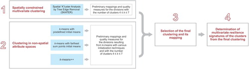
Step 1: spatially constrained multivariate clustering

For the spatially constrained multivariate clustering, we used Spatial ‘K’luster Analysis by Tree Edge Removal (SKATER). Here, we briefly report on its outcomes (for a full description, see Supplementary Appendix 1).

For this study reported in this article, we intentionally limited the number of clusters to seven to ensure data comprehension and explanation. According to Miller’s law (Miller 1956), mapping more than seven classes may be a demanding task in terms of data interpretation. Therefore, we focused on examining four divisions that had between four and seven clusters. Next, to gain better insights into the four divisions resulting from the SKATER clustering, we iteratively calculated the total WCSS to identify the division with minimum variation within clusters. The resulting values were similar (for more details, see Supplementary Appendix 1).

Step 2: clustering in non-spatial attribute spaces

Clustering and seeding technique

For the clustering in non-spatial attribute spaces, we employed k-means. The method is designed to partition a set of n multidimensional data items (in our case, 428 Norwegian municipalities), where each item is a d-dimensional real vector, into k (≤ n) sets, where k is the number of clusters and d is the number of dimensions (in our case, the 47 resilience indicators). Each k-means algorithm is initialized by seeding (i.e., by selecting initial centroids). Seeding is of utmost importance to any type of k-means clustering because different seeding techniques result in different clustering outcomes. For this reason, in our study, we experimented with three seeding techniques: predefined initial means, farthest sum points initial means, and k-means++. Whereas the first two techniques are more exact, the third is commonly used in k-means clustering.

For our first seeding technique, predefined initial means, we identified the resilience indicator that had the highest average correlation coefficient with the remaining 46 resilience indicators included in the analysis, which was “percent of the population living in urban areas” (URBAN_POP). We then sorted all municipalities in ascending order according to that variable and created k nearly equal partitions by taking the first N/k observations for the first group (where N was the number of municipalities and k the number of clusters), the second N/k observations for the second group, and so on. Finally, we used the centroids of those groups as the initial centroids for the k-means clustering process.

The second seeding technique, farthest sum points initial means, randomly chooses the first initial municipality as the centroid and then repeatedly selects the “farthest” municipality by the sum of distances to already chosen centroids. We ran this technique multiple times with all possible first initial centroids (hence, one run for each of the 428 Norwegian municipalities) and selected the division with the highest performance regarding the quality measure, which was minimum variation within clusters (minimum sums of the squared error).

Lastly, our third seeding technique, k-means++ (Arthur & Vassilvitskii 2007), picks out the first centroid (i.e., municipality) at random from the data points to be clustered, and then each subsequent centroid is chosen from the remaining data points (municipalities), with the probability proportional to its squared distance from the point’s closest existing cluster center. Once initial centroids have been identified, the standard k-means algorithm is executed. However, since different rounds of k-means++ for the same data commonly produce different divisions, we performed five computation sessions, each with 10,000 runs of k-means++. In each computation session, we selected the division with the highest performance regarding the minimum variation within clusters. Although the five sessions resulted in five different divisions, they differed only to a minor extent. We therefore compared how municipalities were classified in the four divisions with four, five, six, and seven clusters (Table 2) and did the final assignment based on the following rule: if a given municipality was assigned at least three times to the same cluster in the five divisions, the municipality was assigned to that cluster. However, this rule did not work for the clustering with seven groups, since two municipalities were assigned to the same cluster only twice. Therefore, for that clustering, we repeated the computation session to obtain an extra classification and to assign a cluster to the two municipalities.

Table 2. Classification of municipalities in five computation sessions, each with multiple runs of the k-means++ clustering

	Number of municipalities assigned to the same cluster in five computation sessions
k	5 times	4 times	3 times
4	413 (96%)	15 (4%)	–
5	425 (99%)	–	3 (1%)
6	417 (97%)	8 (2%)	3 (1%)
7	357 (83%)	20 (5%)	51 (12%)

Number of clusters

For each of the seeding techniques, we repeatedly examined the resulting clusters. Moreover, we checked configurations with various cluster numbers. However, for certain divisions, we obtained clusters with only a few elements. Therefore, as with the SKATER clustering (Step 1), we intentionally limited the number of clusters and performed the analysis with four, five, six, and seven clusters. Despite the different seeding techniques and the growing number of clusters, the geographies reflected across the divisions featured similar spatial patterns. The summarized evolution of the k-means clustering process is shown in Fig. 2, in which the maps show the geographies of the divisions resulting from the k-means clustering by seeding technique and number of clusters. In almost all divisions, there is a clear divide between the south and north of Norway. Moreover, there are clearly visible clusters consisting of urban municipalities such as Oslo, Trondheim, and Bergen.

Fig. 2. Evolution of the clustering process with four, five, six, and seven clusters identified through k-means clustering with three different seeding techniques: predefined initial means, farthest sum points initial means, and k-means++

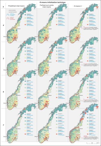
For the divisions with four and five clusters, the distributions of municipalities across the clusters in particular seeding techniques are quite similar, whereas differences become more pronounced for the divisions with six and seven clusters. Particularly distinct are the divisions with six and seven clusters resulting from k-means initiated by farthest sum points initial means. Furthermore, some clusters feature very few municipalities.

Since we could not determine the “best” division resulting from the k-means clustering from visual examination of the maps in Fig. 2, total WCSS was again calculated for all divisions. Moreover, although spatial contiguity was not forced in the k-means, we searched for the clustering that was characterized by the best spatially grouped pattern. Accordingly, for all examined divisions, we also calculated Moran’s I index with the inverse distance (Euclidean distance, row standardization) used to determine spatial relationships between objects. The highest Moran’s I index was observed for the divisions with seven clusters (0.57) and six clusters (0.56), while the lowest WCSS (1780.64) was found for the division with six clusters, both resulting from k-means++ (highlighted in bold in Table 3). This means that the division featured the lowest variability of the observations within clusters; it minimized the within group dispersion and maximized the between-group dispersion. The six-cluster division also performed well regarding the number of municipalities assigned to the same cluster in all five sessions of the k-means++ clustering process. As shown in the far right-hand column in Fig. 2, only 11 municipalities in the division were classified differently during the five sessions. That was the second-best result, after the division with five clusters with only three differently classified municipalities (Table 2).

Table 3. Moran’s I indices and within-cluster sum of squares (WCSS) for the divisions obtained from k-means with predefined initial means, farthest sum points initial means, and k-means++

k	k-means with predefined initial means				k-means with farthest sum points initial means				k-means++
	Global Moran’s I statistic			Total within-cluster sum of squares (WCSS)	Global Moran’s I statistic			Total within-cluster sum of squares (WCSS)	Global Moran’s I statistic			Total within-cluster sum of squares (WCSS)
	Moran’s I index	Z-Score	p		Moran’s I index	Z-Score	p		Moran’s I index	Z-Score	p
4	0.30	14.66	0.000	1785.16	0.37	18.10	0.000	1785.03	0.36	17.65	0.000	1784.55
5	0.32	15.56	0.000	1783.58	0.37	18.13	0.000	1781.36	0.54	26.53	0.000	1783.07
6	0.43	21.26	0.000	1782.02	0.41	20.01	0.000	1783.31	0.56	27.47	0.000	1780.64
7	0.23	11.46	0.000	1781.68	0.21	10.27	0.000	1781.82	0.57	27.99	0.000	1781.38

Step 3: selection of the final clustering and its mapping

To select the final clustering for the further analysis, we considered two options: the “best” divisions from the SKATER clustering and the “winners” of the k-means divisions (Fig. 2). We used Moran’s I index and WCSS to select the final clustering. We also considered the number of municipalities in the clusters, as low differences in terms of municipality counts facilitate data comprehension.

With regard to the SKATER clustering, the division with four clusters performed best in terms of Moran’s I index of spatial autocorrelation (0.95, F = 46.44, p < 0.001), while the highest WCSS score was observed for the division with seven clusters (Supplementary Appendix 1). However, the Moran’s I indices for the k-means++ divisions with seven and six clusters were also respectable (0.57, F = 27.99, p < 0.001 and 0.56, F = 27.47, p < 0.001, respectively). The k-means++ division with six clusters performed best with regard to WCSS, as it had the lowest WCSS score in all checked divisions resulting from both SKATER and k-means. Furthermore, the k-means++ division with six clusters performed better than did the SKATER divisions, considering the more balanced number of municipalities in clusters. It also had fewer municipalities without certain classification compared with the k-means++ division with seven clusters.

The SKATER results were influenced by the imposed neighborhood relationship constraint and were thus not solely dependent on the municipalities’ similarities in terms of their resilience indicator values. Hence, certain areas (e.g., big cities, mountainous municipalities), despite often being similar with respect to their socioeconomic and area resource characteristics, were assigned to different groups because they did not fulfill the spatial contiguity requirement. Considering the imposed constraint and the fact that k-means++ performed reasonably well compared with the SKATER divisions, we judged the k-means++ results more suitable for further analysis than other considered divisions and therefore chose it for our final clustering.

To examine the geographies of the selected final clustering, we mapped its six clusters jointly and individually. The individual maps highlighted the distinct spatial patterns of the clusters. In addition, we dissected the clusters with regard to the number of municipalities, size (area and population), and area resource classification.

Step 4: determination of multivariate resilience signatures of clusters

To gain insights into the multivariate characteristics of the clusters, we determined their multivariate resilience signatures. To identify and visualize the signatures, we used Jacques Bertin’s reorderable matrix (Bertin 1967). The matrix is an analysis and visualization method for the exploration of multidimensional data by encoding the matrix’s cell values visually and using the matrix’s reordering mechanism to group similar rows and columns. The method has been reconsidered by Perin et al. (2014), who have developed the web application Bertifier that enables users to create tabular visualizations from data (Perin et al. n.d.).

First, we calculated the clusters’ mean values for all 47 resilience indicators (Supplementary Appendix 2). Next, we assigned each cluster ranks, based on the following rule: the higher the mean value of a cluster, the higher the assigned rank (Supplementary Appendix 2). The rankings were then imported into the Bertifier web application. We used Bertifier to visualize the ranks using Bertin’s matrix: for each indicator, the clusters were encoded to range from no symbol, which corresponded to the lowest rank, to the biggest symbol (a square), which corresponded to the highest rank; the intermediate clusters were encoded with circles. Bertifier was next used to reorder the matrix to find distinct patterns embedded in the graphically encoded indicator ranks. The patterns in the matrix’s columns reflected the multivariate resilience signatures of the clusters. Next, differences between the multivariate signatures of the clusters were explored. We also calculated the overall ranks of the resilience subdomains (i.e., social, economic, institutional, infrastructure & housing, community capital, and environmental) by adding their respective indicators’ ranks.

Results: examination of the geographies and multivariate resilience signatures of one cluster division

The geographies of the k-means++ clustering with six clusters

The six groups of municipalities resulting from the selected k-means++ clustering are shown summarized in Fig. 3.³ Clusters F and A, which represented antipodal regions in Norway (Fig. 4) included the fewest municipalities, whereas the most numerous clusters were C and D. With regard to territory, with the exception of Clusters E and F, which were the smallest and almost equal in terms of territory, the remaining clusters differed considerably. The largest cluster, which also had the highest number of municipalities, was C (Fig. 4). The differences in terms of population were even bigger. While less than 2% of the population lived in the least populated cluster, A, more than 50% of Norwegian citizens lived in the most populated cluster, F. The largest cluster, C, was home to only 4% of the population. Hence, the two least inhabited clusters were A and C, which had similar proportions of population to territory (population density).

Fig. 3. Summary of the six groups of Norwegian municipalities resulting from the six-group k-means++ clustering

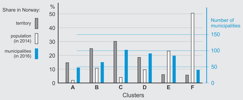
Fig. 4. Norwegian municipalities clustered on the basis of their similarities in terms of their community resilience indicators

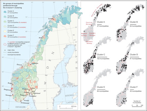
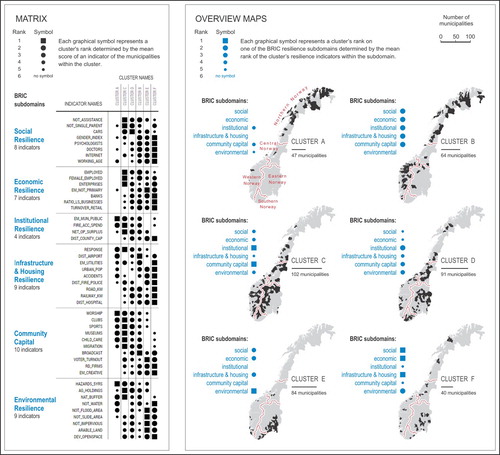
Although certain clusters were characterized by well-shaped spatial patterns (Fig. 4), their division did not fit specific regions and only the northernmost and the least populated cluster, A, encompassed municipalities that were mostly located in Northern Norway; only 4 of its 47 municipalities were located elsewhere. In turn, the 64 municipalities of Cluster B were more scattered than those in Cluster A. Nevertheless, most of them were concentrated in Northern Norway (22) and Western Norway (35). Municipalities belonging to Cluster C were scattered throughout the whole country, but most of them were concentrated in the country’s inland area in south-west Norway. Similarly, municipalities in Cluster D were scattered throughout the whole country. Lastly, the two last clusters, E and F, were the most specific of all clusters: they covered the least territory but were the most populated clusters. Cluster E constituted the most spatially consistent region, as it mainly comprised municipalities concentrated around the capital, Oslo, in the south-east. However, its municipalities were also concentrated around several Norwegian cities along the coast, such as Kristiansand, Stavanger, Haugesund, Bergen, Ålesund, and Trondheim (see the map to the left in Fig. 4). Whereas Cluster E could be described as a suburban cluster, Cluster F was urban, and corresponds to the major urbanized areas in Norway, including the biggest urban settlements in the north, Bodø and Tromsø.

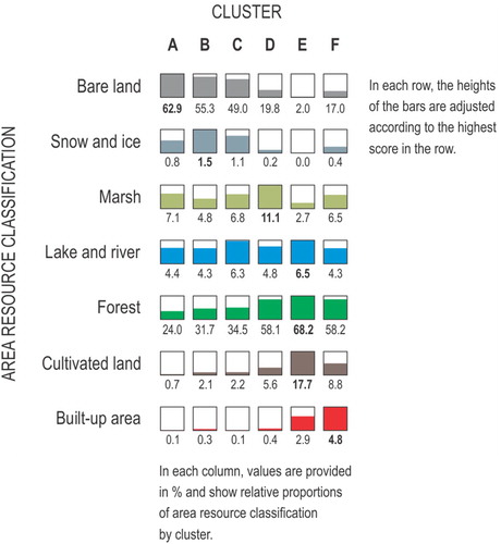
To elicit further how land cover types defined the clusters, we examined the cluster division with regard to the official area resource classification used by the Norwegian Institute of Bioeconomy Research (Solberg et al. 2019). The classification includes criteria for vegetation, natural drainage and cultural impact. We calculated the shares of various area resource types in each cluster. Figure 5 depicts the relative proportions between clusters. The geographies of the six clusters were well reflected in the shares. For example, Cluster C consisted of many mountainous municipalities across the whole country, most of them with exposed and elevated areas. Its area therefore featured higher shares of bare land, snow, and ice than did Cluster D’s area. By contrast, the latter cluster (D) — also scattered throughout Norway — consisted of many lower lying municipalities and therefore Cluster D contained a higher share of marsh and forest. Cluster E, which comprised municipalities concentrated around the biggest cities, featured the highest share of forest and cultivated land, whereas Cluster F, which had urbanized municipalities, had the highest share of built-up area.

Fig. 5. Relative proportions of area resource classification by cluster

Multivariate resilience signatures

Reorderable matrix

The matrix in Fig. 6 summarizes the resilience indicators of the final clusters. In the matrix, the clusters (columns) are graphically encoded by the resilience indicators (rows); the latter are grouped into the six community resilience subdomains. The symbols represent each cluster’s rank for the specific indicator (row), determined by the mean score on the indicator of the municipalities in the cluster. The ranks range from no symbol (blank), which indicates the lowest rank (the lowest mean score), to the square symbol that depicts the highest rank (the highest mean score). Each cluster is thus assigned an individual multivariate signature composed of a set of graphical symbols. To facilitate visual examination and, most importantly, to highlight differences between clusters, we reordered the matrix’s columns and rows (within subdomains). For each cluster, we also calculated an overall rank for each subdomain (based on the sum of ranks) (shown next to the overview maps in Fig. 6).

Fig. 6. The multivariate signatures of the six groups of municipalities found similar in terms of their resilience to natural hazards

Multivariate resilience signatures of clusters

The two geographically antipodal clusters, A and F, were classified oppositely in the matrix (Fig. 6). Their antipodal nature applied to all six subdomains (i.e., if one cluster featured higher performance relative to other clusters in one subdomain, the other cluster featured the opposite). Hence, Clusters A and F differed not only because of their geographic distance and population density, but also because of their socioeconomic and environmental characteristics.

In most subdomains, Cluster A featured the lowest performance. Its overall ranking was the lowest with regard to the social, economic, and infrastructure & housing resilience subdomains. In total, it scored lowest on 21 out of 47 resilience indicators. However, for three indicators, Cluster A scored highest of all clusters. On average, municipalities within Cluster A had higher proportions of the labor force working in public administration and services, including the defense sector (EM_MUN_PUBLIC), compared with municipalities in other clusters. Additionally, there were more religious institutions per 1,000 persons (WORSHIP), and fewer loss-causing natural hazard events in the 5-year period prior to 2014 (HAZARDS_5YRS).

Cluster B featured relatively higher performance than other clusters in five of the six subdomains. The only exception was the environmental resilience subdomain, for which it scored poorest among all clusters. Overall, it scored poorest on only two indicators: (1) percentage of the land area not prone to landslides (NOT_SLIDE_AREA), indicating that municipalities within the cluster were somewhat landslide prone (due to a substantial share of bare land, snow, and ice; see Fig. 5); and (2) proximity to fire and police stations (DIST_FIRE_POLICE), indicating that the mean distances to public safety providers from urbanized settlements (tettsteder) within the cluster were greater than the distances within other clusters. Cluster B also had the highest performance on two indicators: proximity to airports (DIST_AIRPORT), and the number of broadcasters per 1,000 persons.

Overall, Cluster C scored highest in the institutional resilience and community capital subdomains. On an individual indicator basis, it was diverse, as it had the highest performance on 15 indicators and the lowest performance on 7 indicators. In the social resilience subdomain, municipalities within Cluster C had on average a smaller proportion of their population dependent on social assistance (NOT_ASSISTANCE) and fewer single-parent households (NOT_SINGLE_PARENT). On a negative note, there seemed to be a lack of medical professionals (DOCTORS), and a smaller proportion of the population was of working age. In the economic resilience subdomain, Cluster C municipalities portrayed higher average employment rates (EMPLOYED) than did municipalities within other clusters, as well as a higher average rate of female labor force participation (FEMALE_EMPLOYED), and a greater number of enterprises per 1,000 persons (ENTERPRISES). However, they featured the lowest performance relative to other clusters with regard to employment outside the primary sector and tourism, which indicated that many people depended on those sectors for their livelihoods.

The high score of Cluster C in the institutional resilience subdomain was supported by two financial indicators: municipal spending on fire and accident prevention (FIRE_ACC_SPEND) and municipal net operating surplus (NET_OP_SURPLUS). In the infrastructure & housing resilience subdomain, Cluster C did not fare too well: on average, it was the least urbanized cluster (URBAN_POP), with the greatest distances to airports (DIST_AIRPORT). However, it had the highest performance on one indicator: on average, there were more fire, police, ambulance stations, and shelters per 1,000 persons (RESPONSE) in the cluster than in any other cluster. In the community capital subdomain, Cluster C’s best overall rank was driven by the five highest scoring indicators and one high scoring indicator. On average, municipalities in the cluster had higher performance relative to other clusters with regard to cultural and community services, such as religious institutions (WORSHIP), youth clubs (CLUBS), sports facilities (SPORTS), museums (MUSEUMS), and childcare institutions (CHILD_CARE) per 1,000 persons, as well as with regard to in-migration and out-migration (MIGRATION), thus indicating it had a more stable population compared with other clusters. In the environmental resilience subdomain, Cluster C municipalities on average had more agricultural holdings per 1,000 persons (AG_HOLDINGS) and more land area covered by natural flood buffers (NAT_BUFFER), such as marshes, than did municipalities in other clusters. However, the municipalities were also more prone to flooding (NOT_FLOOD_AREA) on average and had more water bodies and rivers (NOT_WATER) compared with other clusters.

Cluster D was a “midfielder” in terms of overall and individual indicator ranks. Overall, it had neither the lowest nor the highest performance in any subdomain. It had the highest mean score for cars per 1,000 persons (CARS), but it featured the highest mean score for traffic accidents (ACCIDENTS).⁴ Cluster D had on average the lowest performance on the gender equality index (GENDER_INDEX).

Overall, Cluster E (the “suburban cluster”) was the “winner” in the environmental subdomain, but the “loser” in the institutional resilience and community capital subdomains. It ranked first in six indicators, mostly in the environmental resilience subdomain, and last in eight indicators, mostly in the community capital subdomain. Cluster E’s excellent performance in the environmental resilience subdomain was due to four indicators, for which it scored highest, and one indicator, for which it scored fairly high. Municipalities within this cluster were on average less prone to flooding (NOT_FLOOD_AREA) and landslides (NOT_SLIDE_AREA), had smaller areas covered by impervious surfaces (NOT_IMPERVIOUS), and had larger areas dedicated to agricultural production (ARABLE_LAND) and classified as developed open space (DEV_OPENSPACE) compared with municipalities in other clusters. However, Cluster E municipalities ranked last in natural flood buffers (NAT_BUFFER).

In the infrastructure & housing resilience subdomain, it became evident that a relatively larger part of the population of Cluster E lived in urban settlements (URBAN_POP) compared with in other clusters. Cluster E municipalities scored highly on road safety (ACCIDENTS), as they had fewer accidents per 1,000 persons than did other cluster municipalities. They also scored highly on proximity to fire and police stations (DIST_FIRE_POLICE) and hospitals (DIST_HOSPITAL). However, municipalities in Cluster E seemed to lack adequate funding for accident and fire prevention (FIRE_ACC_SPEND) as they had the lowest performance with regard to that resilience indicator. In the community capital subdomain, Cluster E had the lowest performance relative to other clusters with regard to childcare institutions (CHILD_CARE) and cultural resources such as museums (MUSEUMS). In addition, it ranked last with regard to in-migration and out-migration (MIGRATION), thus indicating a degree of fluctuation within the population. However, it had a higher performance relative to other clusters with regard to sources of innovation (RD_FIRMS, EM_CREATIVE) and the highest performance with regard to voter turnout (VOTER_TURNOUT), which indicates a highly educated and politically engaged population. Not surprisingly, in the economic resilience subdomain, Cluster E excelled in having a large part of its labor force working outside the primary sector and tourism (EM_NOT_PRIMARY). Moreover, there were fewer people working in public utilities (EM_UTILITIES) and other public services (EM_MUN_PUBLIC) compared with other clusters. In the social resilience subdomain, Cluster E has only one poorest indicator; on average, its municipalities had more single-parent households (NOT_SINGLE_PARENT) than municipalities in other clusters.

Lastly, Cluster F (the “urban cluster”) ranked first in the social, economic, and infrastructure & housing resilience subdomains, and second in the environmental resilience subdomain. It outperformed all other clusters by ranking highest on 20 of 47 indicators and second highest on a further 8 indicators. In the social resilience subdomain, it scored highest on access to healthcare services (DOCTORS, PSYCHOLOGISTS), access to communication (INTERNET), gender equality (GENDER_INDEX), and working age population (WORKING_AGE). In the economic resilience subdomain, there were on average more enterprises (ENTERPRISES) and banks (BANKS) per 1,000 persons located in Cluster F than in the other clusters. There were also more large enterprises (RATIO_LS_BUSINESSES), a higher retail turnover per capita (TURNOVER_RETAIL), and fewer people working in the primary sector and tourism (EM_NOT_PRIMARY).

In terms of institutional resilience, Cluster F did not do very well. Although the cluster scored highest with regard to proximity to county capitals (DIST_COUNTY_CAP), which is not surprising given that it contained many county capital municipalities, it scored lowest with regard to municipal net operating surplus (NET_OP_SURPLUS), which was an indicator of the financial health of the municipality. In the infrastructure & housing resilience subdomain, Cluster F was the clear “winner,” as it scored highest on seven out of nine indicators. It had higher performance relative to other clusters regarding all but the physical response capacity (RESPONSE), as on average there were fewer fire, police, and ambulance stations and fewer shelters per 1,000 persons in the cluster than in any other cluster. With regard to the community capital subdomain, Cluster F was similar to Cluster E. As it was home to a highly skilled and politically engaged population, it scored highly on the indicators relating to sources of innovation (RD_FIRMS, EM_CREATIVE) and voter turnout (VOTER_TURNOUT). However, unlike cluster E, it scored highly on broadcasters per 1,000 persons (BROADCAST). Environmentally, Cluster F had a higher performance relative to other clusters on six out of nine indicators. Municipalities in the cluster were less prone to landslides (NOT_SLIDE_AREA) and floods (NOT_FLOOD_AREA), had smaller areas covered by water bodies (NOT_WATER) and impervious surfaces (NOT_IMPERVIOUS), and had more land under agricultural production (ARABLE_LAND) and classified as developed open space (DEV_OPENSPACE).

Discussion

Key findings

Although the k-means++ clustering is free of spatial contiguity constraints, the geographies of the six resulting regions featured relatively well-kept spatial patterns (Fig. 4), and the regions were meaningful and interpretable in the Norwegian context. For example, although scattered throughout Norway, urban municipalities were grouped into the “urban cluster,” F. In turn, the “northern cluster,” A, comprised municipalities that were mostly in the northernmost part of Norway. Another pattern was the concentration of the municipalities from Cluster E around major cities. Those municipalities accompanied Cluster F and were therefore termed the “suburban cluster.” Cluster C comprised many low-populated municipalities along the mountain divide between Western Norway and Eastern Norway.

Municipalities with the highest scores on resilience indicators were grouped mainly in Clusters F and C. The “urban cluster,” F, scored highest on 20 indicators (see the matrix in Fig. 6) and was by far the most resilient cluster in the infrastructure & housing resilience subdomain. In the social resilience subdomain, it scored highest with regard to features typical of urban areas, such as numbers of doctors and psychologists. Finally, from Cluster F’s high scores in the economic resilience subdomain, it is clear that the cluster encompassed wealthy municipalities. In terms of shortcomings, its municipalities had low performance relative to other clusters in terms of community capital and in the institutional resilience subdomain. However, many of the community capital indicators were calculated as per 1,000 persons and could thus have been biased toward rural low-populated municipalities. With regard to the institutional resilience subdomain, many smaller municipalities with fewer people had higher municipal income levels than did more populated urbanized areas (Regjeringen 2018; Pedersen 2018), which affected the two financial indicators in the subdomain. In turn, 15 indicators supported the overall success of municipalities in Cluster C, 7 of which belonged to the institutional resilience and community capital subdomains. The reasons for Cluster F’s low performance in these two subdomains were cluster C’s gains. Four indicators in the community capital subdomain were “per 1,000 persons,” which boosted Cluster C municipalities’ indicator values and subsequent rank assignments. Many of the Cluster C municipalities were wealthy rural municipalities (in terms of municipal income), and some were prosperous tourist destinations for winter sports activities.

Although we did not intend to stigmatize any particular region of Norway, as often is the unintentional result of indexation exercises such as those done by Holand et al. (2011), Rød et al. (2015), and Scherzer et al. (2019), Northern Norway yet again seemed to fare poorest. The northern cluster, A, was ranked lowest in almost half of the considered resilience indicators and in contrast to the “urban cluster,” F, it scored lowest in the social, economic, and infrastructure & housing resilience subdomains. The number and diversity of recognized potential shortcomings in Northern Norway, as highlighted by both this and other studies (Holand et al. 2011; Rød et al. 2015; Scherzer et al. 2019), need further examination. Detailed qualitative research could provide valuable insights into specific issues, which in turn could facilitate local interventions and mitigation strategies.

Practical application

Climate change adaptation may be a challenging task for many Norwegian municipalities, especially for small municipalities with limited human and economic resources. Knowledge of neighboring or nearby municipalities that have similar challenges may make it easier for municipalities to form networks that could promote learning and shared actions towards building more resilient communities.

This raises the question as to how the findings of our clustering exercise could be used in practice. Local decision-makers need to identify their municipalities’ less resilient qualities when facing potentially damaging events and to design strategies to improve them (IFRC 2016). In addition to existing municipal risk and vulnerability analyses,⁵ municipalities with similar resilience characteristics could benefit from exchanging knowledge, even if they are remote and feature different environmental conditions. If a group of municipalities exhibits shortcomings regarding certain resilience indicators, those shortcomings could be investigated across the group and ultimately lead to targeted interventions that could apply to the whole group or parts of the group, rather than to individual municipalities. Possibly, that would result in more effective mitigation efforts, as costly interventions could be implemented simultaneously in a number of municipalities. Moreover, decision-makers and practitioners in the field of disaster preparedness and management could benefit from having an overview of the geographies of regions comprising municipalities with similar resilience signatures, as specific measures could be targeted at groups of geographically near municipalities that have similar needs in terms of certain resilience indicators.

Studies that construct new indices and groupings are frequently conducted at a high level of abstraction, with diverse data aggregated for large areas. Hence, their outcomes often outline the bigger picture, providing an overview at a municipal, regional, or national scale. While findings from such studies may be translated into practical information, they should in most cases serve as starting points for further analysis, especially since most indicators serve as proxies for something else. For example, in the community capital subdomain, the indicators SPORTS, CLUBS, and WORSHIP serve as proxies for certain aspects of community involvement, and low performance on these indicators, such as recorded for Clusters E and F, should not trigger immediate actions to improve them. The indicators themselves are an imperfect choice and the result of data availability constraints. Rather than measuring the numbers of sports facilities, youth clubs, or religious institutions per 1,000 persons, it would have been better to include actual numbers of membership or affiliation for those indicators—data that unfortunately are unavailable. Nonetheless, it may seem a reasonable result that indicators of community involvement were lower in urban areas than in rural areas. However, if the objective is to improve community involvement in urban areas, another study with a different methodology is needed. For example, qualitative methods such as focus groups or interviews could be used to identify operational goals.

Method limitation

It needs to be acknowledged that the indicators, and by extension the resilience dimensions, are often interconnected, statistically and conceptually (for further thoughts on this matter see Scherzer et al. 2019). The indicators and dimensions should therefore not be interpreted in isolation but need to be interpreted considering the entirety of the set of indicators and the wider context of any locality.

Overall, the findings from our study need to be seen within the framing of the original purpose of the data, namely to describe and measure community resilience. Any potential indicator shortcomings need to be evaluated first with regard to the indicator’s intended purpose, efficacy of indicator choice and relation to other indicators, and second with regard to the potential implications for the municipalities. For example, the lowest score for Cluster B on percentage of the land area not prone to landslides (NOT_SLIDE_AREA), meaning Cluster B was fairly landslide prone, was caused by the substantial share of bare land, snow, and ice in the municipalities that constituted the cluster. However, before planning interventions, there is a need to check whether landslide-prone areas are inhabited. In another example, Cluster C had the lowest performance relative to other clusters with regard to employment outside the primary sector and tourism (EM_NOT_PRIMARY). This meant that many people depended on those sectors for their livelihoods, but it does not necessarily mean that interventions were needed.

Conclusions

By exploring the multivariate resilience signatures of the clusters based on their relative strengths or weaknesses on certain indicators, we were able to answer the research question about the differing resilience qualities of the clusters (RQ1). The study revealed four unique and clearly defined clusters (A, C, E, and F), which allowed for a comprehensive interpretation of their community resilience through the unambiguous linking between well-delineated spatial areas and specific resilience signatures. The two remaining clusters, B and D, were thought of as “midfielders,” due to their ambiguity in terms of overall and individual indicator ranks.

With the clustering exercise documented in this study, we have provided suggestions for which municipalities could benefit from forming municipality networks, potentially informing common operational planning toward building more resilient local communities. If a group of municipalities were to score low on a range of indicators, indicating that the municipalities were less resilient than other municipalities, common actions could be undertaken to investigate the shortcomings further, and, if found necessary, shared targeted interventions could be planned and knowledge exchanged. By targeting several municipalities simultaneously, for example those from the “urban cluster” F or those from the “suburban cluster” E, interventions could become more efficient than if they were organized separately in individual municipalities.

The method applied in our study to examine a pre-existing dataset of community resilience indicators fitted well within the body of research in which cluster analysis was employed to reveal patterns in multidimensional geographical data. Importantly, we extended the typical cluster analysis approach by employing Bertin’s reorderable matrix (Bertin 1967) to gain better insights into the outcomes of the clustering exercise. Follow-up studies are needed to verify whether this method, combining a clustering technique with Bertin’s reorderable matrix, is applicable to other datasets (i.e., transferrable to other contexts), especially those involving indicators intended to measure multifaceted concepts.

Lastly, further research is needed on community resilience. Although this concept has already attracted extensive scientific attention, its implications for mitigation actions in Norway have so far been insufficiently studied, especially considering the re-emerging deficiencies of Northern Norway.

Acknowledgements

We are grateful to the editors for inviting excellent referees and to the referees for providing thoughtful comments on earlier versions of the article. We also thank the members of the ClimRes project team (Gunhild Setten, Haakon Lein, Silje Aurora Andresen, and Aleksi Räsänen) as well as Ivar Holand and Per Arne Stavnås for useful discussions on the relevance of the selected indicators. Additionally, we thank the participants of a departmental seminar in which the early steps and the preliminary outcomes of the cluster analysis were presented. Last but not least, we are grateful to Catriona Turner for language editing and for providing us with valuable suggestions on our article.

Additional information

Funding

This work was supported by the project “Climate change, and natural hazards: The geography of community resilience in Norway” (ClimRes), funded by the Research Council of Norway’s KLIMAFORSK program (Grant number NRC 235490). It was also supported by the Research Council of Norway's funding for research stays abroad (Grant number NRC 250028).

Notes

1 All reverse-scaled variables are marked with an asterisk in Table 1.

2 In Norway, an urban settlement can comprise as few as 60–70 buildings inhabited by at least 200 persons if the distance between the buildings does not exceed 50 m, although exceptions may apply (Statistics Norway 2020).

3 We used data from the Norwegian Mapping Authority to calculate the shares of clusters of Norway’s entire territory and data from Statistics Norway to calculate the shares of population.

4 ACCIDENTS is a reverse-scaled indicator serving as a proxy measure of road safety. A high (low) score on this indicator relates to a low (high) average number of traffic accidents per 1,000 persons.

5 All Norwegian municipalities are required to perform a risk and vulnerability analysis (risiko- og sårbarhetsanalyse, ROS).

References

- Arthur, D. & Vassilvitskii, S. 2007. k-means++: The advantages of careful seeding. SODA ‘07: Proceedings of the Eighteenth Annual ACM-SIAM Symposium on Discrete Algorithms, 1027–1035. https://dl.acm.org/doi/abs/10.5555/1283383.1283494 (accessed 1 April 2014).
- Aldrich, D.P. 2012. Building Resilience: Social Capital in Post-Disaster Recovery. Chicago, IL: University of Chicago Press.
- Aldrich, D.P. & Meyer, M.A. 2015. Social capital and community resilience. American Behavioral Scientist 59, 254–269. doi: 10.1177/0002764214550299
- Barnett, J., Lambert, S. & Fry, I. 2008. The hazards of indicators: Insights from the Environmental Vulnerability Index. Annals of the Association of American Geographers 98, 102–119. doi: 10.1080/00045600701734315
- Bertin, J. 1967. Sémiologie Graphique. Paris: Editions Gauthier-Villars.
- Bohman, A., Neset, T.S., Opach, T. & Rød, J.K. 2014. Decision support for adaptive action – assessing the potential of geographic visualization. Journal of Environmental Planning and Management 58, 2193–2211. doi: 10.1080/09640568.2014.973937
- Burton, C.G. 2015. A validation of metrics for community resilience to natural hazards and disasters using the recovery from Hurricane Katrina as a case study. Annals of the Association of American Geographers 105, 67–86. doi: 10.1080/00045608.2014.960039
- Cai, H., Lam, N.S.N., Qiang, Y., Zou, L., Correll, R.M. & Mihunov, V. 2018. A synthesis of disaster resilience measurement methods and indices. International Journal of Disaster Risk Reduction 31, 844–855. doi: 10.1016/j.ijdrr.2018.07.015
- Cox, R.S. & Hamlen, M. 2015. Community disaster resilience and the Rural Resilience Index. American Behavioral Scientist 59, 220–237. doi: 10.1177/0002764214550297
- Cullum, C., Brierley, G., Perry, G.L.W. & Witkowski, E.T.F. 2017. Landscape archetypes for ecological classification and mapping: The virtue of vagueness. Progress in Physical Geography: Earth and Environment 41, 95–123. doi: 10.1177/0309133316671103
- Cutter, S.L. 2016. The landscape of disaster resilience indicators in the USA. Natural Hazards 80, 741–758. doi: 10.1007/s11069-015-1993-2
- Cutter, S.L., Mitchell, J.T. & Scott, M.S. 2000. Revealing the vulnerability of people and places: A case study of Georgetown County, South Carolina. Annals of the Association of American Geographers 90, 713–737. doi: 10.1111/0004-5608.00219
- Cutter, S.L., Boruff, B.J. & Shirley, W.L. 2003. Social vulnerability to environmental hazards. Social Science Quarterly 84, 242–261. doi: 10.1111/1540-6237.8402002
- Cutter, S.L., Barnes, L., Berry, M., Burton, C., Evans, E., Tate, E. & Webb, J. 2008. A place-based model for understanding community resilience to natural disasters. Global Environmental Change 18, 598–606. doi: 10.1016/j.gloenvcha.2008.07.013
- Cutter, S.L., Burton, C.G. & Emrich, C.T. 2010. Disaster resilience indicators for benchmarking baseline conditions. Journal of Homeland Security and Emergency Management 7. doi: 10.2202/1547-7355.1732
- Cutter, S.L., Ash, K.D. & Emrich, C.T. 2014. The geographies of community disaster resilience. Global Environmental Change 29, 65–77. doi: 10.1016/j.gloenvcha.2014.08.005
- Delmelle, E.C. 2016. Mapping the DNA of urban neighborhoods: Clustering longitudinal sequences of neighborhood socioeconomic change. Annals of the American Association of Geographers 106, 36–56. doi: 10.1080/00045608.2015.1096188
- Flanagan, B.E, Gregory, E.W., Hallisey, E.J., Heitgerd, J.L. & Lewis, B. 2011. A social vulnerability index for disaster management. Journal of Homeland Security and Emergency Management 8. doi: 10.2202/1547-7355.1792
- Fotheringham, A.S., Brunsdon, C. & Charlton, M. 2000. Quantitative Geography: Perspectives on Spatial Data Analysis. London: SAGE.
- Frazier, T.G., Courtney M.T. & Dezzani, R.J. 2014. A framework for the development of the SERV model: A spatially explicit resilience-vulnerability model. Applied Geography 51, 158–172. doi: 10.1016/j.apgeog.2014.04.004
- Grubesic, T.H. & Murray, A.T. 2001. Detecting Hot Spots Using Cluster Analysis and GIS. https://www.researchgate.net/profile/Alan_Murray6/publication/228883015_Detecting_Hot_Spots_Using_Cluster_Analysis_and_GIS/links/541d68120cf203f155bf1662.pdf (accessed 1 April 2020).
- IFRC. 2016. World Disasters Report: Resilience: Saving Lives Today, Investing for Tomorrow. Geneva: International Federation of Red Cross and Red Crescent Societies.
- Holand, I.S., Lujala, P. & Rød, J.K. 2011. Social vulnerability assessment for Norway: A quantitative approach. Norsk Geografisk Tidsskrift–Norwegian Journal of Geography 65, 1–17. doi: 10.1080/00291951.2010.550167
- Jennings, P.J. 2008. Using cluster analysis to define geographical rating Territories. [Casualty Actuarial Society (ed.)] 2008 Casualty Actuarial Society Discussion Paper Program: Applying Multivariate Statistical Models, 34–52. https://www.casact.org/pubs/dpp/dpp08/08dpp.pdf (accessed 1 April 2020).
- Kaufman, L. & Rousseeuw, P.J. 2009. Finding Groups in Data: An Introduction to Cluster Analysis. Hoboken, NJ: John Wiley.
- Lam, N.S.N., Reams, M., Li, K., Li, C. & Mata, L.P. 2016. Measuring community resilience to coastal hazards along the northern Gulf of Mexico. Natural Hazards Review 17(1): 04015013. doi: 10.1061/(ASCE)NH.1527-6996.0000193
- Leuprecht, A. & Gobiet, A. (2010). Classification of Precipitation Regions in the Alpine Area Using Cluster Analysis. Scientific Report No. 35-2010. Graz: Wegener Center.
- Mahlstein, I. & Knutti, R. 2010. Regional climate change patterns identified by cluster analysis. Climate Dynamics 35, 587–600. doi: 10.1007/s00382-009-0654-0
- Mayunga, J.S. 2007. Understanding and Applying the Concept of Community Disaster Resilience: A Capital-based Approach. https://www.theisrm.org/documents/Mayunga%20(2007)%20Understanding%20and%20Applying%20the%20Concept%20of%20Community%20Disaster%20Resilience%20-%20A%20Capital-Based%20Aproach.pdf (accessed 1 April 2020).
- Mihunov, V.V., Lam, N.S.N., Zou, L., Rohli, R.V., Bushra, N., Reams, M.A. & Argote, J.E. 2018. Community resilience to drought hazard in the south-central United States. Annals of the American Association of Geographers 108, 739–755. doi: 10.1080/24694452.2017.1372177
- Miles, S.B. & Chang, S.E. 2011. ResilUS: A community based disaster resilience model. Cartography and Geographic Information Science 38, 36–51. doi: 10.1559/1523040638136
- Miller, G.A. 1956. The magical number seven, plus or minus two: Some limits on our capacity for processing information. Psychological Review 63, 81–97. doi: 10.1037/h0043158
- Norris, F.H., Stevens, S.P., Pfefferbaum, B., Wyche, K.F. & Pfefferbaum R.L. 2008. Community resilience as a metaphor, theory, set of capacities, and strategy for disaster readiness. American Journal of Community Psychology 41, 127–150. doi: 10.1007/s10464-007-9156-6
- OECD-JRC. 2008. Handbook on Constructing Composite Indicators: Methodology and User Guide. Paris: OECD.
- Peacock, W.G. (ed.) 2010. Advancing the Resilience of Coastal Localities: Developing, Implementing and Sustaining the Use of Coastal Resilience Indicators: A Final Report. https://www.researchgate.net/profile/Walter_Peacock/publication/254862206_Final_Report_Advancing_the_Resilience_of_Coastal_Localities_10-02R/links/00b7d51feb3e3d0d4a000000.pdf (accessed 1 April 2020).
- Pedersen, O.P. 2018. Her er de rikeste og fattigste kommunene. KommunalRapport. https://kommunal-rapport.no/okonomi/2018/05/her-er-de-rikeste-og-fattigste-kommunene (accessed 11 March 2020).
- Perin, C., Dragicevic, P. & Fekete, J.-D. 2014. Revisiting Bertin’s matrices: New interactions for crafting tabular visualizations. IEEE Transactions on Visualization and Computer Graphics 20, 2082–2091. doi: 10.1109/TVCG.2014.2346279
- Perin, C., Dragicevic, P. & Fekete. J.-D. n.d. Bertifier. https://aviz.fr/bertifier_app/ (accessed 26 February 2019).
- Petschel-Held, G., Block, A., Cassel-Gintz, M., Kropp, J., Lüdeke, M.K.B., Moldenhauer, O., Reusswig, F. & Schellnhuber, H.J. 1999. Syndromes of global change: A qualitative modelling approach to assist global environmental management. Environmental Modelling Assessment 4, 295–314. doi: 10.1023/A:1019080704864
- Pfefferbaum, R.L., Pfefferbaum, B., Van Horn, R.L., Klomp, R.W., Norris, F.H. & Reissman, D.B. 2013. The Communities Advancing Resilience Toolkit (CART): An intervention to build community resilience to disasters. Journal of Public Health Management and Practice 19, 250–258. doi: 10.1097/PHH.0b013e318268aed8
- Regjeringen. 2018. Frie inntekter korrigert for utgiftsbehov. https://www.regjeringen.no/no/tema/kommuner-og-regioner/kommuneokonomi/inntektssystemet-for-kommuner-og-fylkeskommuner/utgiftskorrigerte-frie-inntekter/id547765/ (accessed 11 April 2018).
- Rød, J.K., Opach, T. & Neset, T.-S. 2015. Three core activities toward a relevant integrated vulnerability assessment: Validate, visualize, and negotiate. Journal of Risk Research 18, 877–895. doi: 10.1080/13669877.2014.923027
- Rose, A. 2004. Defining and measuring economic resilience to disasters. Disaster Prevention and Management: An International Journal 13, 307–314. doi: 10.1108/09653560410556528
- Rose, A. 2007. Economic resilience to natural and man-made disasters: Multidisciplinary origins and contextual dimensions. Environmental Hazards 7, 383–398. doi: 10.1016/j.envhaz.2007.10.001
- Rose, A. & Krausmann, E. 2013. An economic framework for the development of a resilience index for business recovery. International Journal of Disaster Risk Reduction 5, 73–83. doi: 10.1016/j.ijdrr.2013.08.003
- Ritchie, L.A. & Gill, D.A. 2006. Social capital theory as an integrating theoretical framework in technological disaster research. Sociological Spectrum 27, 103–129. doi: 10.1080/02732170601001037
- Scherzer, S., Lujala, P. & Rød, J.K. 2019. A community resilience index for Norway: An adaptation of the Baseline Resilience Indicators for Communities (BRIC). International Journal of Disaster Risk Reduction 36: 101107. doi: 10.1016/j.ijdrr.2019.101107
- Sempier, T.T., Swan, D.L., Emmer, R., Sempier, S.H. & Schneider, M. 2010. Coastal Community Resilience Index: A Community Self-Assessment: Understanding How Prepared your Community Is for a Disaster. http://masgc.org/assets/uploads/publications/662/coastal_community_resilience_index.pdf (accessed 5 March 2017).
- Sherrieb, K., Norris, F.H. & Galea, S. 2010. Measuring capacities for community resilience. Social Indicators Research 99, 227–247. doi: 10.1007/s11205-010-9576-9
- Sietz, D., Lüdeke, M.K.B. & Walther. C. 2011. Categorisation of typical vulnerability patterns in global drylands. Global Environmental Change 21, 431–440. doi: 10.1016/j.gloenvcha.2010.11.005
- Sietz, D., Ordoñez, J.C., Kok, M.T.J., Janssen, P., Hilderink, H.B., Tittonell, P. & van Dijk, H. 2017. Nested archetypes of vulnerability in African drylands: Where lies potential for sustainable agricultural intensification? Environmental Research Letters 12, 095006. doi: 10.1088/1748-9326/aa768b
- Singh-Peterson, L., Salmon, P., Goode, N. & Gallina, J. 2014. Translation and evaluation of the baseline resilience indicators for communities on the Sunshine Coast, Queensland Australia. International Journal of Disaster Risk Reduction 10, 116–126. doi: 10.1016/j.ijdrr.2014.07.004
- Solbjørg, E., Heggem, F., Mathisen, H. & Frydelund, J. 2019. AR50 – Arealressurskart i målestokk 1:50 000: Et heldekkende arealressurskart for jord- og skogbruk. NIBIO Rapport Vol. 5, no. 118. https://nibio.brage.unit.no/nibio-xmlui/bitstream/handle/11250/2626573/NIBIO_RAPPORT_2019_5_118.pdf?sequence=2&isAllowed=y (accessed 1 April 2020).
- Statistics Norway. 2020. Tettsteders befolkning og areal, 1. januar 2016. https://www.ssb.no/befolkning/statistikker/beftett/aar/2016-12-06?fane=om (accessed 7 February 2020).
- Tate, E. 2012. Social vulnerability indices: A comparative assessment using uncertainty and sensitivity analysis. Natural Hazards 63, 325–347. doi: 10.1007/s11069-012-0152-2
- Tierney, K. 2012. Disaster governance: Social, political, and economic dimensions. Annual Review of Environment and Resources 37, 341–363. doi: 10.1146/annurev-environ-020911-095618
- Twigg, J. 2009. Characteristics of a Disaster-resilient Community: A Guidance Note. Teddington: DFID Disaster Risk Reduction NGO Interagency Group.
- UNDP 2014. Understanding Community Resilience: Findings from Community-based Resilience Analysis (CoBRA) Assessments. Nairobi: UNDP Drylands Development Centre. http://www.undp.org/content/dam/undp/library/Environment%20and%20Energy/sustainable%20land%20management/CoBRA/CoBRA_Assessments_Report.pdf (accessed 6 March 2017).
- Yoon, D.K., Kang, J.E. & Brody, S.D. 2016. A measurement of community disaster resilience in Korea. Journal of Environmental Planning and Management 59, 436–460. doi: 10.1080/09640568.2015.1016142