Diversity and distribution of landscape types in Norway

ABSTRACT

Norwegian landscapes are changing at an increasingly rapid rate and therefore systematically structured information about observable landscape variation is required for knowledge-based management of landscape diversity. The purpose of the article is to present the first version of a complete, area covering, evidence-based, landscape type map of Norway, simultaneously addressing geoecological, bioecological and land use related variations. The type system used for the mapping is supported by systematically structured empirical evidence. The results of the mapping procedure, including the geographical distribution and descriptive statistics (abundance and areal coverage), are presented for each of the nine identified major landscape types identified based on coarse-scale landform variation. Within six inland and coastal major types, a large number of minor landscape types are defined based on the composition of geoecological, bioecological, and land use related landscape properties. The results provide new insights into the geography of Norwegian marine, coastal and inland landscapes. The authors discuss potential errors, uncertainties and limitations of the landscape type maps, and address the potential value of the new tool for research, management and planning purposes. They conclude that the results of the study might contribute to knowledge-based spatial planning and management of the unique landscape diversity of Norway.

KEYWORDS:

• landscape diversity
• landscape mapping
• landscape type
• Norway

Introduction

Landscape characterisation and mapping in Norway

Norway is widely recognised as a ‘hot spot’ of European landscape diversity (Mücher et al. 2010; Ciglič & Perko 2013), as it comprises an exceptional range of variation in climatic conditions, bedrock, landforms, vegetation, and land use within a relatively small area (Moen 1999; Bakkestuen et al. 2008). In common with most other European countries (Plieninger et al. 2016), landscapes in Norway are changing at an increasingly rapid rate (Eiter & Pothoff 2007). Since the development of land use policies often implies choices between irreconcilable views on the desired utilisation of a landscape, there is a growing demand for planning and management strategies that combine the protection of landscape diversity with sustainable use of landscape resources. Systematically structured information about observable landscape variation is a prerequisite for knowledge-based spatial planning and landscape management (Marsh 2005) and essential for the fulfilment of obligations set by international conventions such as the European Landscape Convention (Council of Europe 2020), which was ratified by Norway in 2004. Moreover, the aim of Norway’s Nature Diversity Act (Ministry of Climate and Environment 2009) is to protect ‘biological, geological and landscape diversity’ and promote conservation and sustainable use of the ‘full range of variation of habitats and landscape types’ throughout the nation. This goal presupposes knowledge about the abundance and spatial distribution of ‘landscape types’.

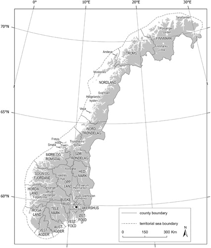
The conceptual idea of assigning landscapes to types is rooted in the tradition of systematic physical geography or ‘landscape geography’, the aim of which is to present and explain typologies of similar landscapes based on their material content (Holt-Jensen 2018). Because processes related to geomorphology, ecology and human land use are tightly intertwined, many landscape elements tend co-vary in predictable and recurrent patterns throughout larger regions (R.G. Bailey 2009). This is exemplified by a mountain plain in Hardangervidda (Buskerud county), which is more similar to a distant mountain plain in Valdresflye (>100 km north-east, in Oppland county) or even in Finnmarksvidda (>1000 km north-east, in Finnmark county) than to any of the valleys surrounding the plain with respect to its content of landforms, ecosystems and other landscape elements (Fig. 1).¹ Accordingly, grouping similar landscapes into types is an effective way to communicate landscape information because affiliation to type alone will provide an extensive amount of information about any individual of that particular type. Since a type in a type system comprises a predictable and ‘normal’ amount of landscape variation, affiliation to type is also a useful reference and a good starting point for assessment of the unique character and properties of individual landscapes (e.g. Phillips 2007).

Fig. 1. Location of counties in 2018 and other places in Norway

The concept of landscape types has been used informally in geographical and ecological literature in Norway since the early 20th century (e.g. Nordhagen 1943; Sømme 2008 [1938]). Earlier landscape type maps are coarse in scale and based on a priori defined key variables rather than systematically structured evidence (e.g. Thorsnes et al. 2009; Erikstad & Blumentrath 2011; Buhl-Mortensen et al. 2015). To date, comprehensive and evidence-based landscape type maps have not been established for Norway. Other national landscape characterisation efforts have followed a regional geographical tradition by identifying and describing the individual character of particular landscape areas (i.e. by identifying landscapes or regions with a high degree of internal similarity). Notable earlier efforts within the regional geographical tradition include interpretative and holistic approaches (e.g. Nordisk Ministerråd 1987; Puschmann 2005), as well as more observer-independent, data-driven methods (e.g. Strand 2011; Krøgli et al. 2015). Geographical landscape analyses at the regional scale have served as a useful framework for several applied purposes (Strand 2011). Nevertheless, these analyses have lacked the thematic and spatial resolution necessary to serve as a relevant knowledge base for land use policies and environmental impact assessments (EIAs) at the local–regional scale (i.e. c.1:50,000) (e.g. Helland et al. 2015). Most governmental guidelines for landscape analysis recommend a mainly value-neutral description of the observable properties of a landscape as a starting point for character, value and suitability assessments based on context-specific criteria (e.g. Helland et al. 2015, Statens vegvesen 2018). To ensure better quality and consistency of general landscape descriptions, several Norwegian scientists have called for a more systematic, observer-independent and repeatable framework as a reference and a knowledge base for a multitude of applied purposes (e.g. Moen 1999; Strand 2011; Erikstad et al. 2015; Krøgli et al. 2015).

EcoSyst – a new framework for systematisation of nature diversity

To meet the need for more detailed, systematic, observer-independent, and area covering information about Norway’s nature’s diversity as required by the Nature Diversity Act, the Norwegian Biodiversity Information Centre (NBIC) started development of the project ‘Nature in Norway’ (NiN) in 2005 (Halvorsen et al. 2016). NiN has since been developed into a universal theoretical framework for systematisation of nature’s diversity, EcoSyst, which simultaneously addresses biotic and abiotic variation across different levels of organisation from ecosystem components to landscapes (Halvorsen et al. 2020).

Since the term ‘landscape’ is understood and applied differently within the disciplines that have landscape as a subject of interest (e.g. geography, geology, geomorphology, ecology, history, archaeology, and landscape architecture (Jones & Stenseke 2011)), any attempt to systematise variation at the landscape level requires a clear definition of the term ‘landscape’. In the EcoSyst framework, landscape is recognised as a separate level of ecological diversity, simultaneously addressing biotic and abiotic variation in heterogeneous areas of kilometres-wide extent (Noss 1990) (see also definitions of key concepts in Appendix 1). The EcoSyst framework addresses the material properties of the landscape, defined as a more or less uniform area characterised by its content of observable, natural and human-induced landscape elements (Halvorsen et al. 2020). ‘Landscape elements’ are defined as ‘natural or human-induced objects or characteristics, including spatial units assigned to types at an ecodiversity level lower than the landscape level, which can be identified and observed on a spatial scale relevant for the landscape level of ecodiversity’ (Halvorsen et al. 2020, 1889). ‘Landscape types’ are defined as reoccurring units more or less uniform areas characterised by their content of observable, natural and human-induced landscape elements (Halvorsen et al. 2020).

As a first step towards a new Norwegian landscape type map based upon EcoSyst principles (Supplementary Appendix S1), a pilot NiN landscape typology was developed for Nordland county (Erikstad et al. 2015). Based on the experience gained from the Nordland pilot, the study area was expanded to encompass the entire country (Simensen et al. 2020a). Based on statistical analyses of landscape variation in a sample of observation units (landscapes) throughout Norway (Simensen et al. 2020a), a tentative, abstract (i.e. non-spatial) landscape typology was established.

However, few patterns in ecology make sense unless viewed in an explicit geographical context (Lomolino et al. 2017). This article answers to the challenge of translating the abstract EcoSyst (NiN) landscape typology of Simensen et al. (2020a) into the first version of a complete, area covering, evidence-based, landscape type map for Norway. We accomplish this aim by applying simple map algebra operations to publicly available geographical data sets with full areal coverage of Norway. Furthermore, we present the results of the mapping, including the geographical distribution and descriptive statistics (abundance and areal coverage) for each of the identified landscape types. Finally, we discuss potential errors, uncertainties and limitations of the landscape type maps and we address the potential value of this new tool for research, management and planning purposes.

Materials and methods

Study area

The studied area spans 57°57′N to 71°11′N and 4°29′E to 31°10′E, which comprises the entire mainland of Norway, including the coastal zone (landscapes with coastline) and marine areas (i.e. completely submerged under marine water). The range of variation in natural conditions found in Norway includes most of the variation found in the circumboreal zone (Bryn et al. 2018), including terrestrial, marine, limnic, and snow and ice ecosystems (Halvorsen et al. 2016). All seven bioclimatic temperature-related vegetation zones commonly recognised in northern Europe, from boreo-nemoral to high alpine, occur in Norway (Bakkestuen et al. 2008). Norway has a high mineral and bedrock diversity, and a high diversity of landforms (Gjessing 1978; Ramberg et al. 2008). The diversity of Norwegian landscapes is enhanced by historical land use such as domestic grazing, outfield fodder collection, heath burning, reindeer husbandry, forestry, and industrial, urban and recreational development (Almås et al. 2004; Hansen & Olsen 2004; Jacobsen & Follum 2008).

Source data

All source data used to derive the landscape type maps were obtained from publicly available geographical data sets with full areal coverage of Norway (Table 1). The basis data consisted of (1) continuous variables (e.g. digital elevation model (DEM)), (2) categorical landscape and land-cover data (e.g. AR 50² land cover types), and (3) point and line data (e.g. buildings and infrastructure). All spatial data were either converted to raster format with a resolution of 100 × 100 m or adapted to this grain size by resampling or rasterisation from vector formats. We obtained the DEM by combining a terrestrial DEM interpolated from 20 m height contour lines (N50 topographic maps³) with a marine DEM (bathymetric data, 50 m resolution). For 275 of the freshwater lakes in the study area, bathymetry data were available from the Norwegian Water Resources and Energy Directorate, while for the remaining freshwater lakes >2 km² we interpolated the bathymetry by inverse distance weighting based on DEM values for the terrestrial surroundings (Supplementary Appendix S6). Finally, terrestrial, marine and freshwater DEMs were combined to a seamless DEM and adapted to 100 m resolution by spatial aggregation (Rød 2015).

Table 1. Baseline input map layer information

Abbreviation	Theme/dataset	Description	Variable category	Original map scale/raster resolution	Data provider
DEM	Digital elevation model (DEM)	The terrain model is a grid model with a resolution (grid size) of 100 × 100 m.	Continuous	20 m interval contour lines	NMA
N50	Topographic map	General purpose topographic map, including land cover (e.g. water, soil type), administrative areas, buildings and facilities, height, restricted areas, transport and communications, and place names	Discrete	1:50,000	NMA
AR50	Land cover	Land Resource Map, scale 1:50,000 The national land resource database (AR) classifies the land cover of mainland Norway according to its suitability for agriculture and natural plant production.	Discrete	1:50,000	NIBR
PF	Potential forest	A high-resolution GIS null model of potential forest expansion following land use changes in Norway, including forest line and boreal heaths	Discrete	25 m	NIBR
ESWM	Wave exposure	Wave index model of the Norwegian coast (Isæus 2004), based on distance to nearest shore, average wind speed and wind frequency	Continuous	25 m	IMR
R_net	Hydrology	River network database, watercourses	Discrete	1:50,000	NVE
GAB	Buildings	The official Norwegian register of buildings and properties registered in the land register	Point data	1:50,000	NMA

Notes: NMA – Norwegian Mapping Authority; NIBR – Norwegian Institute of Bioeconomy Research; IMR – Institute of Marine Research; NVE – The Norwegian Water Resources and Energy Directorate

Overall methodological approach

The overall methodological approach included two main stages: analysis and mapping. First, detailed analyses of landscape variation in a sample of observation units (landscapes) were conducted and the results used to derive a type system. With some adaptions, this type system was used as the platform on which a rule-based, semi-automated procedure for mapping the entire study area was built. The empirical basis for the landscape type system applied in this article is multivariate analyses of 85 landscape variables collected in a stratified sample of 100 test areas (25 × 25 km) covering 56,400 km² (about one-sixth of mainland Norway (Simensen et al. 2020a)). In addition to serving as the empirical basis for a tentative type system, these analyses provide general knowledge about the distribution of landscape elements throughout Norway (Simensen et al. 2020a). Within ‘major landscape types’, primarily defined by coarse-scale landform variation, a unique set of ‘complex landscape gradients’ (CLGs) was identified. A CLG is defined as an ‘abstract, continuous variable that expresses more or less gradual, co-ordinated change in a set of more or less strongly correlated landscape variables’ (Halvorsen et al. 2020, 92). Examples of CLGs are represented by gradual variation in landscape properties from inner to outer coast, gradual variation in vegetation cover from lowlands to barren mountains, and gradual variation in landscape element composition due to variation in human land use. A novel procedure to quantify the similarities between different landscapes (‘ecodiversity distance’) was applied (Halvorsen et al. 2020). The tentative, abstract (i.e. non-spatial) landscape typology was derived by combining segments along sets of CLGs specific to each major type.

Modelling landscape gradients

Based on the source data, we derived the variables that were used to identify CLGs by multivariate statistical analyses and subsequently to develop the tentative landscape type hierarchy described by Simensen et al. (2020a). The process by which the CLGs and landscape types were ‘translated’ into spatially explicit proxies (i.e. maps) involved three different approaches:

1. direct spatial projection of variables used in the statistical analyses of landscape variation

2. application of well-documented GIS algorithms that replicated (spatially) the results from the statistical analyses (e.g. geomorphometric analyses (Hengl & MacMillan 2009))

3. development of new geocomputation methods to derive spatial proxies for the identified complex landscape gradients.

Back-transformation of values from the statistical analyses allowed for refining of criteria for separation between major types based on identified important terrain characterising variables such as relative relief and the proportion of flat terrain within a larger area.

Derived variables used for modelling were obtained either by reclassification and filtering of categorical land cover data or by continuous neighbourhood calculations, also referred to as ‘focal statistics’ (Lovelace et al. 2019) or as a ‘moving window’ (Cushman et al. 2010). Focal statistics consider a central cell and its neighbours within a specified distance (window). The window moves over the landscape, one cell at a time, calculating the selected metric (e.g. sum) within the window (neighbourhood) and returning that value to the focal cell (Supplementary Appendix S2). Our goal was to address landscape variation corresponding to the spatiotemporal domain defined by Dikau (1989) as ‘meso-scale’ (i.e. abiotic and biotic patterns occurring at spatial scales of approximately 10⁶–10¹⁰ m² in response to processes operating at temporal scales of 10¹–10⁴ years). Therefore, we used a neighbourhood circle with a radius of 3000 m around the processing cell to derive coarse-scale geomorphometric variables, as recommended by Pike et al. (2009). We derived fine-scale geomorphometric variables and continuous land cover variables by focal statistics using a radius of 500 m (Pike et al. 2009) (Table 2; Supplementary Appendixes S3–S5).

Table 2. Complex landscape gradients (CLGs) with short descriptions

Code	Complex landscape gradient	Description	Functional variable category	Number of segments	Major type group	Major type	Data source	Geocomputation	Detailed descriptions
KLG-RE-IA	Relief in hills and mountains	Terrain-form variation within inland hill and mountain landscapes; from depressions in hills and mountains (RE-IA·1), via undulating inland hills and mountains (RE-IA·2), moderately rugged hills and mountains (RE-IA·3) and rugged hills and mountains (RE-IA·4) to steep and rugged hills and mountains (RE-IA·5)	Geoecological	5	Inland	IA	DEM	MA; focal; vrm; Tpi; RR; recl.	Appendix S5.2
KLG-RE-ID-KF	Relief in valleys and fjords	Terrain-form variation within inland valley and coastal fjord landscapes; as expressed by the depth-to-width ratio of the valley/fjord relative to its surroundings; from wide fjord/valley (RE-KF·1) via open fjord/valley (RE-KF·2) and narrow fjord/valley (RE-KF·3) to deeply cut fjord/valley (RE-KF·4)	Geoecological	4	Inland, coast	ID,KF	DEM	MA; focal; recl.	Appendix S5.2
KLG-RE-KS	Relief in coastal plains	Terrain-form variation within coastal plains from flat (RE-KS·1) (RE-KS·2) coastal plains to rugged coastal plains, often with remnant peaks (RE-KS·3)	Geoecological	3	Coast	KS	DEM	MA; focal; RR; reclass	Appendix S5.3
KLG-IYK	Inner-outer coast	Variation in coastal landscapes, from areas with ‘inland properties’ on the mainland-facing side of larger islands, rarely exposed to the harsh conditions of the open sea (protected inner coast; IYK·1), to the outer coast, directly exposed to the actions of wind, waves and ocean currents (strongly wave-exposed outer coast; IYK·5); the intermediate segments are moderately protected coast (IYK·2), moderately wave-exposed coast (IYK·3), and wave-exposed outer coast (IYK·4)	Geoecological	4	Coast	KS	ESWM, N50 R_net	MA; focal; Log-tr.; reclass.	Appendix S.5.4
KLG-KA	Distance to coast	Variation in inland landscape properties from near-coastal inland plains (situated <5 km from the coastline) to inland plains in the interior of the land mass.	Geoecological	2	Inland	IS	AR50	MA; reclass	Appendix S5.5
KLG-IP	Abundance of lakes	Variation within valleys from landscapes without lakes or with small lakes only (IP·1; all lakes <2 km^2), via valleys with medium-sized lakes (IP2·1; lakes 2–8 km^2), to valleys with large lakes, typically ‘inland fjords’ (IP2·1; >8 km²)	Geoecological	3	Inland	ID	N50	MA: reclass	Appendix S5.6
KLG-VP	Abundance of wetlands	Variation within inland landscapes in the areal cover of wetland (including mires) and the abundance of small lakes and tarns (which are often associated with wetlands): from low–medium abundance (VP·1) to high abundance (VP·2)	Geoecological	2	Inland, coast	IS,KF,KS	N50	MA; focal; recl.	Supp. Append. S5.7
KLG-BP	Glacier presence	Variation in the presence of glacier(s); BP·1: glacier absent; BP·2: glacier present	Geoecological	2	Inland	IA,IS, ID	AR50	MA; recl.	Supp. Append. S5.8
KLG-VE	Vegetation cover	Variation in vegetation cover from forested or potentially forested areas below the climatic forest line (VE·1) to barren mountains, without or with sparse vegetation cover (VE·4): the intermediate segments are: boreal heath-dominated areas below the climatic forest line, kept open due to historical land use with logging and grazing (VE·2) and open mountain heaths (VE·3)	Bioecological	4	Inland, coast	IA,IS,ID, KF	AR50, PF	MA; recl.	Suppl Append.S5.9
KLG-AI	Land use intensity	Variation in the impact of human infrastructure (agricultural land use excepted) from low (AI·1) and intermediate (AI·2) to settlement (village or small town; AI·3) and city (AI·4), expressed by an index (range: 0–13.2) that integrates the abundances of buildings, roads and other visible signs of human infrastructure	Land use related	4	Inland, coast	IA,IS,ID,KF,KS	GAB N50	Focal; recl.	Supp. Append.S5.10
KLG-JP	Agricultural land use intensity	Variation in expressed agricultural land use intensity, from low (JP·1) to high (JP·2)	Land use related	2	Inland, coast	IA,IS,ID,KF,KS	N50	Focal; recl.	Supp. Append. S5.11

Notes: Code – CLG term in Norwegian (NBIC 2019); KA – coastal hills and mountains; KF – coastal fjords; KS – coastal plains; IA – inland hills and mountains; ID – inland valleys; IS – inland plains; Data – original geodata used for geocomputation (see Table 1); Geocomputation – geocomputation methods; MA – map algebra; focal – focal raster calculations; Vrm – vector ruggedness measure; Tpi – topographic position index; RR – relative relief; Log-tr. – Log-transformation; reclass – reclassification; Supp. Append. – reference to detailed description of geocomputation method in Supplementary Appendix (supplementary data online)

Delineation of major landscape types

Supported by the statistical analyses, we assigned spatial landscape units to one of the three major type groups by their relation to the coastline (Fig. 2). ‘Coastal landscapes’ were identified as landscapes at the interface between the land and marine environments; all landscape units that contained a segment of the continuous coastline of a land area were assigned to the coastal landscapes ‘major type’ group. We assigned the spatial landscape units to major type group by zonal operations identifying presence of marine, coastal and terrestrial pixels (Rød 2015).

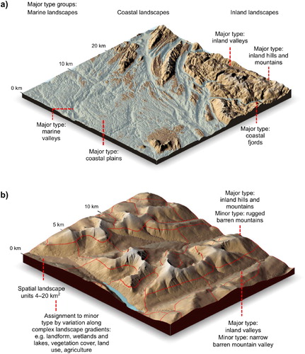
Fig. 2. Landscape type units at different levels in the landscape type hierarchy: a) marine, coastal, and inland and landscapes on Helgelandskysten (Nordland county), with examples of major landscape types; b) major types, minor types and spatial landscape units (red lines) in Rondane (Oppland county)

The statistical analyses (Simensen et al. 2020a) supported recognition of three meso-scale landforms in coastal and inland Norway: ‘plains’, ‘hills and mountains’ and ‘fjord and valleys’. We identified these landform types by geomorphometric calculations based upon the DEM. We first delineated valleys and fjords by focal DEM calculations, using 3 km neighbourhoods. Our fjord and valley model (described in detail in Supplementary Appendix S4) identified elongated depressions in the terrain by application of the algorithms ‘terrain position index’ (TPI) (Gallant & Wilson 2000), the ‘Top Hat approach’ – including ‘valley index’ and ‘valley depth’ (Rodriguez et al. 2002), and ‘peak- and ridge detection’ (Jasiewicz & Stepinski 2013) (for further details, see Supplementary Appendixes S3 and S4). Valleys and fjords were then split into two major types according to their location relative to the coastline by converting identified valleys to vector data and selecting features by their relationships to the coastline and subsequently applying a cost-distance calculation (Supplementary Appendix S4). Valleys completely submerged under marine water were then assigned to the major type ‘marine valleys’.

‘Coastal plains’ were defined as landscapes with coastline (not already defined as valleys and fjords), situated within ±50 m above/below sea level. This pragmatic morphometric definition largely encompasses the strandflat⁴ (Gjessing 1978; Sulebak 2007), as well as other coastal areas with low relief. The elevation criterion (±50 m) was operationalised by requiring that >0.5 of all cells within 1 km neighbourhoods were situated in that interval. Delimitation of ‘coastal plains’ on the inland side was made by applying a cost-distance grid. We applied the same procedure to identify ‘inland plains’, defined as terrestrial landscapes (without coastline) and marine plains (entirely submerged by seawater), by requiring height differences (relative relief) <50 m within a 1 km neighbourhood. Due to the highly variable quality of available soil type maps, we decided not to delineate ‘fine-sediment plains’ as a separate major type in this first version of the landscape type map, although such plains were tentatively identified as a major type on its own in the statistical analyses (see the section ‘Discussion’). After delineating fjords, valleys, and inland and coastal plains, all remaining areas were defined as ‘hills and mountains’. We then merged the major types onto one map and joined areas below the minimum polygon size (4 km²) with adjacent polygons, according to the procedures outlined in Supplementary Appendix S4. Finally, polygons of hills and mountain were assigned to the ‘major type’ group and major type based upon their location relative to the coastline.

Calculation of positions along complex landscape gradients

We developed spatially explicit proxies (i.e. maps) for the 11 CLGs identified in the statistical analyses (Table 2). Three types of proxies were developed: (1) indices based on focal statistics; (2) indices based on the presence or absence of landscape elements; and (3) composite indices (e.g. obtained as the sum of two or more indices, quantifying and weighing the frequencies of landscape elements and properties). We derived proxies for the three geoecological CLGs related to ‘relief’ within coastal plains, coastal fjords, inland valleys and inland hills and mountains, respectively, by morphometric terrain surface calculations based on the DEM (Appendixes S5.1–3). We calculated positions along the CLG ‘inner-outer coast’ as a weighted sum of three elements: (1) amount/abundance of rivers, (2) island size, and (3) wave exposure (Supplementary Appendix S5.4). The CLG ‘distance to coast’ separated near-coastal inland plains from other inland plains and positions were obtained as the Euclidean distance from the nearest coastline-pixel. We used 5 km to the coastline as the threshold for separating ‘near-coastal’ from other inland plains (Supplementary Appendix S5.5). ‘Abundance of lakes’ was calculated by classification of lake size into three classes: small lakes <2 km²; medium-sized lakes 2–8 km² and large lakes >8 km² (Supplementary Appendix S5.6). Calculations of positions along the CLG ‘abundance of wetlands’ was derived from combining focal calculations of wetlands and point data for small lakes (Supplementary Appendix S5.7). The CLG ‘glacier presence’ was obtained directly from reclassification of land cover data (Supplementary Appendix S5.8). We derived the bioecological CLG ‘vegetation cover’ by reclassification of land cover classes from AR50 (obtained from NIBIO). The reclassified model was then combined with the GIS model for ‘potential forest’ (Bryn et al. 2013) (for a reclassification scheme, see Supplementary Appendix S5.9). Positions along the CLG ‘Land-use intensity’ were calculated by a weighted summation of focal calculations of (a) buildings and (b) technical infrastructure (Supplementary Appendix S5.10). Positions along the CLG ‘agricultural land-use intensity’ was obtained by focal calculations of arable land derived from AR50 (Supplementary Appendix S5.11).

The spatial models for the complex landscape gradients followed the results of the statistical analyses closely. Still, a few deviations and adaptions had to be introduced to enhance mapping functionality. In order to account for ‘extreme’ landscape variation along CLGs that was absent or represented with very few observation units in the sample of observation units used for the statistical analyses, we subjectively introduced four new segments along three CLGs to account for landscape elements that dominate the landscape where they are present: AI·3 (village or small town); city (AI·4); high agricultural land use intensity (JP·2); and glacier presence (BP·2).

Delineation of spatial landscape units and assignment to minor landscape types

A method for segmentation of the target area into concrete spatial landscape units is integrated into the process of mapping landscape types, as outlined in EcoSyst (Halvorsen et al. 2020). Adaptation of a landscape type system for mapping at a specific scale implies setting a minimum polygon size. Spatial landscape units represent the most detailed units in the landscape type system and contain individual landscape areas that are homogeneous with respect to terrain properties and landform characteristics. These units are subsequently assigned to types based on landscape element composition. Based on the results of the pilot project in Nordland (Erikstad et al. 2015), the minimum polygon size for the spatial landscape units was set to 4 km². Within each major landscape type, we delineated spatial landscape units by a rule-based division of the landscape into discrete spatial units for subsequent classification into landscape types (Fig. 2). We used ridge lines, inflexion points and other breaking points in the terrain curvature to delineate spatial landscape units that are maximally homogeneous with respect to terrain properties and landform characteristics. For this purpose, we adapted and applied methods for delineation of drainage basins (Horton 1932; Gruber & Peckham 2009), adjusted to the scale of our analysis (spatial landscape units from 4–20 km²). Within areas with mainly convex landforms (e.g. hills and mountains), we applied the same procedure on an inverted DEM. This was motivated by our intention to identify areas that share terrain surface properties rather than delimit entities that are purely hydrological (e.g. a mountain top (for details, see Supplementary Appendix S6)). The landforms identified in our study largely resemble commonly applied classifications of macro- and meso-scale landforms (e.g. plains, hills and mountains) based on surface geometry (cf. Dikau 1989; Sulebak 2007).

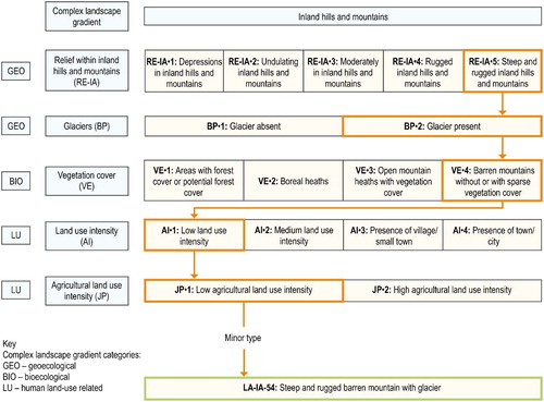
We assigned segments along relevant CLGs to spatial landscape units by summarising values for each CLG within each spatial landscape unit. For this purpose, we used zonal statistics with majority calculations, or by registering the abundance of specific landscape elements within each spatial landscape unit. For example, when the majority (i.e. >50%) of the pixels in a polygon (landscape unit) belonged to segment RE·5 within the CLG ‘relief in hills and mountains’, (i.e. steep and rugged hills and mountains), the spatial landscape unit was coded accordingly. We finally obtained the minor landscape types by map algebra, by adding relevant segments along all CLGs for each major landscape type (Supplementary Appendix S7). Every unique combination of segments along CLGs identified as important for the major type in question was, by definition, considered as one landscape type (Fig. 3) (for details, see Supplementary Appendixes S7 and S8).

Fig. 3. Assignment of spatial landscape units to minor landscape types within a major type

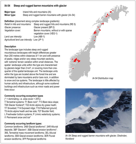
The raster grids with type codes for all polygons for each major type were transformed from raster data to polygons and merged to a complete landscape type map with complete areal coverage for the mapping area. The landscape types were given specific codes (e.g. IA-1, IA-2, and so forth) and descriptive names based on the presence of expected content of landscape elements and CLG position (e.g. ‘steep and rugged mountains with glacier’ (see Table 3 and Supplementary Fig. S9). We generated textual descriptions of each minor landscape type by concatenating text strings with textual descriptions of each segment in CLGs included in each type. We described commonly occurring landscape elements (i.e. ecosystem types and landforms) for each minor type based on three sources: (1) the statistical analyses by Simensen at al. (2020a); (2) data from distribution modelling of ecosystem types (Horvath et al. 2019; Simensen et al. 2020b); and (3) our own expert assessments.

Table 3. Total area of the ten most common minor landscape types within each major type (marine landscapes not included)

Code	Major and minor landscape types	Spatial landscape unit (n)	Total area, km^2	Area in % of major type	Area in % of total area
KS	Coastal plains	4476	36,249	100.0	10.0
KS-44	Very wave-exposed outer undulating coastal plain	844	6489	17.9	1.8
KS-57	Extremely wave-exposed outer undulating coastal plain	720	5811	16.0	1.6
KS-9	Sheltered inner flat coastal plain	674	5140	14.2	1.4
KS-27	Moderately wave-exposed undulating coastal plain	634	4870	13.4	1.3
KS-38	Very wave-exposed outer flat coastal plain	218	1962	5.4	0.5
KS-52	Extremely wave-exposed outer flat coastal plain	198	1775	4.9	0.5
KS-11	Sheltered inner undulating coastal plain with village/small town	176	1419	3.9	0.4
KS-21	Moderately wave-exposed flat coastal plain	124	1064	2.9	0.3
KS-1	Sheltered inner coastal plain	69	641	1.8	0.2
KS-29	Moderately wave-exposed undulating coastal plain with village/small town	76	596	1.6	0.2
KS	Other coastal plains (53 minor types)	743	6482	17.9	1.8
KF	Coastal fjords	3713	33,478	100.0	9.0
KF-9	Open fjord with settlements/infrastructure	1060	9659	28.9	2.6
KF-8	Relatively open fjord	1003	9134	27.3	2.5
KF-17	Narrow fjord	587	4933	14.7	1.3
KF-18	Narrow fjord with settlements/infrastructure	267	2354	7.0	0.6
KF-2	Open fjord with settlements/infrastructure	219	2066	6.2	0.6
KF-1	Open fjord	175	1649	4.9	0.4
KF-11	Relatively open fjord with village/small town	117	1183	3.5	0.3
KF-24	Deeply cut fjord	127	988	2.9	0.3
KF-4	Open fjord with village/small town	48	453	1.4	0.1
KF-20	Narrow fjord with village/small town	27	301	0.9	0.1
KF	Other coastal fjords (16 minor types)	83	758	2.3	0.2
KA	Coastal hills and mountains	74	284	100.0	0.1
KA-1	Coastal hills- and mountains	74	284	100.0	0.1
ID	Inland valleys	11,029	94,607	100.0	25.8
ID-32	Open valley below the forest line	2277	18,202	19.2	5.0
ID-34	Open valley below the forest line with settlements/infrastructure	804	7394	7.8	2.0
ID-1	Wide valley below the forest line	913	7311	7.7	2.0
ID-65	Narrow valley below the forest line	718	5801	6.1	1.6
ID-43	Open barren mountain valley	639	5318	5.6	1.4
ID-38	Open valley with boreal heath below the forest line	516	4213	4.5	1.1
ID-3	Wide valley below the forest line with settlements/infrastructure	420	3843	4.1	1.0
ID-41	Open valley with heath above the forest line	441	3511	3.7	1.0
ID-73	Narrow barren mountain valley	420	3250	3.4	0.9
ID-45	Open valley below the forest line with medium-sized lakes	273	2491	2.6	0.7
ID	Other inland valleys (94 minor types)	3608	33273	35.2	9.1
IA	Inland hills and mountains	21,058	170,523	100.0	46.5
IA-27	Moderately rugged hills below the forest line	2907	22,494	13.2	6.1
IA-14	Undulating hills below the forest line	2585	20,367	11.9	5.6
IA-1	Depressions in hilly landscapes below the forest line	2352	17,388	10.2	4.7
IA-38	Moderately rugged barren mountains	2121	17,384	10.2	4.7
IA-36	Moderately rugged open heath mountains	1351	10,867	6.4	3.0
IA-33	Moderately rugged hills and mountains with boreal heath	1302	10,151	6.0	2.8
IA-53	Steep and rugged barren mountains	1038	8366	4.9	2.3
IA-23	Undulating open heath mountains	926	7464	4.4	2.0
IA-46	Rugged barren mountains	945	6938	4.1	1.9
IA-25	Undulating barren mountains	696	5902	3.5	1.6
IA	Other inland hills and mountains (44 minor types)	4835	4,3202	25.3	11.8
IS	Inland plains	3413	31,834	100.0	8.8
IS-13	Inland undulating plain with wetlands, below the forest line	1005	9763	30.7	2.7
IS-1	Inland undulating plain below the forest line	673	6023	18.9	1.6
IS-10	Inland undulating heath mountain plain	338	2975	9.3	0.8
IS-8	Inland undulating plain with boreal heath, below the forest line	264	2403	7.5	0.7
IS-4	Inland undulating plain with settlements/infrastructure and agriculture, below the forest line	215	2088	6.6	0.6
IS-17	Inland undulating plain with boreal heath and wetlands, below the forest line	148	1521	4.8	0.4
IS-3	Inland undulating plain with settlements/infrastructure, below the forest line	133	1422	4.5	0.4
IS-11	Inland undulating barren heath mountain plain	156	1246	3.9	0.3
IS-18	Inland undulating heath mountain plain with wetlands	81	675	2.1	0.2
IS-22	Coast-near undulating plain with settlements/infrastructure and agriculture, below the forest line	74	559	1.8	0.2
IS	Other inland plains (26 minor types)	326	3159	9.9	0.9

Notes: Code = major type (bold text) and minor type code; major and minor landscape types = descriptive names for major landscape types (bold text) and minor landscape types; spatial landscape units (n) = number of spatial landscape units within each major and minor type.

Quantification of landscape diversity

We quantified landscape diversity for the entire mapping area by calculating the number of landscape types (richness), the number of spatial landscape units of each type (abundance) and the proportion covered by each type within the total mapping area. Richness and abundance cover two aspects of landscape diversity. In very uniform areas such as Finnmarksvidda, large areas will often be assigned to one minor type. In these cases, the number of (adjacent) spatial landscape units will express variation on a finer scale than areal coverage of minor types. We described major spatial patterns of distribution of major and minor landscape types by using terminology (names) of well-known geographical areas, administrative units and bioclimatic gradients (Bakkestuen et al. 2008).

Validation

We compared the theoretical number of types estimated from the sample of observation units (Simensen et al. 2020a) with the final results (realised combinations) obtained by landscape type mapping using the procedures outlined in previous sections. We assessed the consistency and overall quality of the final maps by visual inspection and comparison with high-resolution imagery (orthophotos) and topographic maps (N50), specifically looking for major errors in the delineation and errors in the assignment to segments along each CLG and assignment to major and minor types.

Software

We used ArcGIS Pro (ESRI 2018), and SAGA GIS v.2.3 (O. Conrad et al. 2015) for general geocomputation operations, and R version 3.5.2 for statistical analyses (R Core Team 2018).

Results

The three main results of our study are (1) a hierarchical landscape type system of landscape types in Norway (Fig. 4), (2) complete, area covering, detailed (scale 1:50,000) geographical maps of CLGs and landscape types (Figs. 5 and 6), and (3) estimates of abundance and areal coverage for each major type and the most common minor landscape types (Table 3). Definitions of types and summary statistics for all minor types are provided in Supplementary Appendix S9. Type descriptions and distribution maps for each major and minor type are provided (in Norwegian) by NBIC (2020a; 2020b) (for an example, see Fig. 7).

Fig. 4. ‘Nature in Norway’ project type hierarchy for the landscape level of ecodiversity, with three hierarchical levels: major type groups, major types and minor types (the minor type level has not yet been developed for marine landscapes); the numbers refer to the number of units in each category in the first version of the area covering Norwegian landscape type map

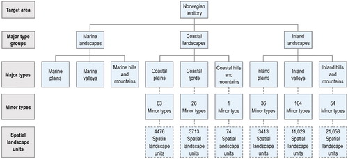
Fig. 5. Examples of complex landscape gradients: a) the geoecological complex landscape gradient ‘relief in coastal plains’ (RE-KS), which expresses terrain form variation within the coastal plains major landscape type, from flat terrain to steep and rugged terrain; b) the bioecological complex landscape gradient ‘vegetation cover’ (VE), which expresses variation from forested or potentially forested areas below the climatic forest line (VE·1) to barren mountains, without or with sparse vegetation cover (VE·4); and c) the land use related complex landscape gradient ‘land use intensity’, expressed by a continuous index (range: 0–13.2) that integrates the abundances of buildings, roads and other visible signs of human infrastructure

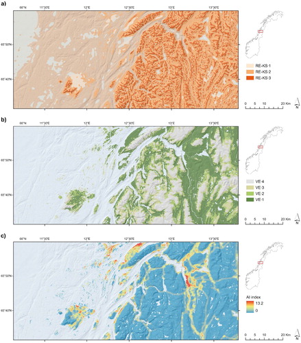
Fig. 6. Selected examples from the ‘Nature in Norway’ project landscape type maps: a) major landscape types differentiated based on broad-scale landforms and terrain variation; b) and c) examples showing major landscape types (indicated by colour), minor landscape types (indicated by codes) and spatial landscape units (delineated by white borderlines) in Moskenes Municipality, in the Lofoten archipelago, Nordland (in map b) and in Romerike, Akershus (in map c)

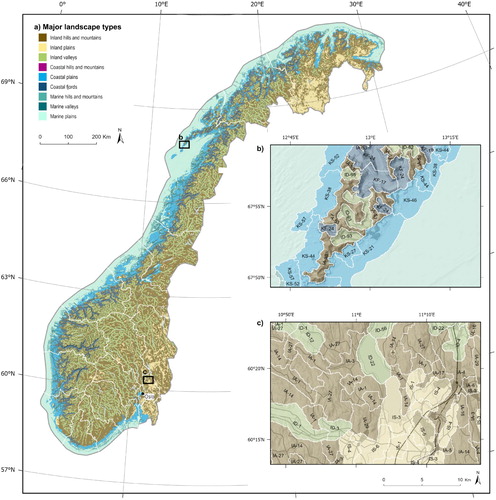
Fig. 7. Example of a landscape type from the landscape database

The highest level of generalisation in the type hierarchy (Fig. 4) contained three ‘major type’ groups. Of the total target area (470,040) km², inland landscapes covered 297,156 km², marine landscapes covered 102,811 km², and coastal landscapes covered 70,073 km².

Level 2 in the type hierarchy consisted of nine major landscape types. Within coastal and inland landscapes, we identified 284 minor landscape types, defined by unique combinations of segments along the 11 CLGs (i.e. with c.8% dissimilarity in landscape element composition between two adjacent minor types). At the most detailed level, we identified 45,640 spatial landscape units (each 2–20 km², with median area 7.4 km², interquartile range 5.4–9.8 km²).

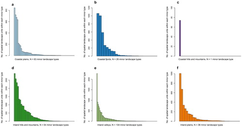
Figure 8 and Supplementary Figs. S9.1–S9.6 show that most of the minor landscape types were represented by <200 spatial landscape units, while only 11 minor types contained more than 1000 spatial landscape units. All major types showed well-defined spatial patterns of distribution related to recognisable and well-known combinations of landscape features. Inland hills and mountains (170,523 km², covering 46.5% of the area of coastal and inland landscapes) were identified as the most common and widely distributed major landscape type throughout Norway (Fig. 6; Table 3). Minor type variation within this major type was related to variation along the CLGs relief, vegetation cover, and land use intensity, resulting in 54 minor types (Fig. 3). The most common and widely distributed minor landscape type in Norway was ‘IA-27 moderately rugged hills below the forest line’, with 2907 spatial landscape units, covering 6.1% of the total inland and mapped coastal area. The maps show a clear and recognizable geographical pattern, with decreasing relief in inland hills and mountains from west to east Norway. The spatial landscape units with high relative relief (IA-RE·5) had a distinct optimum along the western coast, while the optimum for units with low relief (IA-RE·1) was along the Swedish border. At a local scale, there was a significant amount of variation in this broader spatial pattern. Another evident broad-scale pattern with significant local variation was visible in the spatial distribution of the CLG vegetation cover in inland hills and mountains. At a coarser scale, the variation in vegetation cover from forest-covered areas to barren mountains (VE·1–VE·4) mainly followed variation along the two major regional climatic gradients in Norway, from oceanic to continental and from southern/low altitudes to northern/high altitudes. Less common minor types within inland hills and mountains occurred because of infrequent or unique combinations of specific degrees of land use intensity and variation within the geoecological and bioecological gradients. Also, presence of glaciers constitute minor landscape types with relatively few (<100) spatial landscape units.

Fig. 8. The number of spatial landscape units representing each of the 284 minor landscape types within the depicted groups; the minor types are sorted by decreasing number of spatial landscape units (i.e. with one bar representing one minor landscape type, and with common types to the left and rare types to the right)

Inland valleys (94,676 km², 25.8% of the total inland and coastal mapping area) were widely distributed, and the major type comprised high landscape diversity, with 104 minor types, of which only 25 had more than 100 spatial landscape units. The most common minor type was ‘ID-32 open valley below the forest line’ (18,202 km², 2277 spatial landscape units). The variation in relief in valleys followed the same west–east pattern as relief in inland hills and mountains (for examples of valley forms, see Supplementary Appendix S5.2). In addition to relief, vegetation cover, and variations in land use intensity, unique combinations of landscape properties within valleys included minor types defined by the presence of a glacier and types defined by variation in hydrological properties related to lake size.

Inland plains (31,834 km², 8.8% of the total inland and coastal mapping area) were frequent within several disjunct areas; otherwise, they were rare. The most common minor type within inland plains was ‘IS-13 Inland undulating plain below the forest line with wetlands’, which covered large areas in Finnmark, Hedmark and Oppland (1005 spatial landscape units; 9763 km²). ‘Near-coastal inland plains’ (KA·1) occurred on the fringes of the coastal plains along the coast, in the lowlands near Oslofjord (from Østfold to Telemark), in Jæren (Rogaland), on larger islands and in lowland areas near the coast from the Trøndelag region to Nordland and near the coast in eastern Finnmark. Inland plains with large areas of wetlands and lakes (VP·2) were confined to the southern, middle and northern boreal zone, occurring in two distinct areas: (1) the large coastal islands in Trøndelag and Nordland (e.g. Smøla, Hitra and Frøya, Vega and Andøya); and (2) the inland plains in Finnmark and eastern Norway. Further variation in minor types within inland plains followed the variation in regional climate and major soil types and was reflected in variation along the CLGs vegetation cover and (agricultural) land use intensity. Mountain plains (VE·3, VE·4, including premountain plains with boreal heath near the forest line VE·2) occurred in large continuous areas in Finnmarksvidda, the mountain plateau Hardangervidda (Hordaland, Buskerud and Telemark) and as mountain, ‘premountain’ plains (meaning plains near the forest line below the mountains) and forest plains (VE·1) in eastern Norway. Inland plains with high agricultural land use intensity (JP·2) were common in lowland plains in Rogaland (Jæren) and the lowland plains in south-eastern Norway (Vestfold, Østfold, Romerike (Akershus), Toten Municipality (Oppland), Hedemarken (Hedmark), and Glåmdalen south of Elverum Municipality (Hedmark)), also associated with higher land use intensity in general, including minor types with cities and villages (AI·3; AI·4). Distinct and unique minor types included glaciers on inland plains (i.e. plateau glaciers (BP·2), such as Hardangerjøkulen (Hordaland), Svartisen (Nordland) and Folgefonna (Hordaland)).

Coastal plains (36,249 km², 10% of the total inland and coastal mapping area) occurred along the entire length of the coast from Østfold to Finnmark and were particularly well developed in a more than 50 km broad zone in Helgeland (Nordland). The coastal plains encompassed a high number of minor landscape types (63) relative to the total area covered, with variation from inner to outer coast as the most visible geographical pattern. The most common minor type was ‘KS-44 Very wave-exposed outer undulating coastal plains’. Steep and rugged coastal plains with residual mountains (restfjell) had scattered occurrences along the entire coast. Coastal plains with large areas of wetlands and lakes (VP·2) were confined to large coastal island in Trøndelag and Nordland in the southern, middle and northern boreal climatic zone. Coastal plains was the major type with the highest number of spatial landscape units for urban areas. A total of 23 of the 36 spatial landscape units that included a ‘large’ city (64%) were located on coastal plains, while 426 of the 1126 spatial landscape units comprising village, towns and cities (37%) were located in the same major type.

Coastal fjords covered 33,478 km² (9.0% of the total inland and coastal mapping area). Relatively open fjords (RE·2) was the most commonly encountered segment within the relief gradient (2231 spatial landscape units). The most common minor type was ‘KF-9 Relatively open fjord with settlements/infrastructure’, covering 9659 km² (2.6% of the area within inland and coastal landscapes). Coastal fjords was the only major landscape type in which the most common minor type was characterised by a land use intensity above low (AI·1). Six of the most common minor types in fjords had either medium (AI·2) or higher land use intensity. AI·2 typically represented a road along the side of the fjord, with rural settlements and some human land use. Five of the 36 spatial landscape units including a city (14%) were located in fjords.

Coastal hills and mountains (284 km², 0.1% of the total inland and coastal mapping area) were confined to coastal areas between inland hills and mountains and marine areas, not fulfilling the criteria for assignment to either fjords or coastal plains. Coastal hills and mountains were most common in north-western Finnmark, otherwise they occurred scattered along the coast. Due to the low number of spatial landscape units (74) and weak statistical basis for identification of important CLGs, coastal hills and mountains were not divided into minor types.

The most common major marine landscape type in the target area was marine plains (72,948 km², 71.0% of the marine mapping area). This major type encompassed deep marine plains beyond the continental shelf but within the territorial sea boundary, as well as a few marine plains within wide fjord and coastal plain complexes (e.g. Trondheimsfjorden, Porsangerfjorden, Tanafjorden).

Marine hills and mountains (19,493 km², 19% of the marine mapping area) covered the continental shelf off the coastal plains. Marine valleys (10,370 km², 10.1% of the marine mapping area) contained outer parts of fjord systems, either entirely submerged or in deep valleys and gorges that cut through the continental shelf.

The number of realised minor types in the final landscape type map was 284, in contrast to 302 minor types included in the tentative type system derived from statistical analyses (Supplementary Appendix S10). We did not find any misclassification errors in the assignment to types by visual control, but we detected numerous minor delineation irregularities at the most detailed level in the maps (spatial landscape units). We detected minor inconsistencies in assignment to one of the segments along the CLG vegetation cover (KLG-VE (VE-2) in Table 2). Minor delineation irregularities were not quantified or corrected but were noted for later revision with the use of an improved DEM.

Discussion

The new Norwegian landscape type database presented in this article, provides, to our knowledge, the most detailed maps that simultaneously address biotic and abiotic variation at the landscape level of ecological diversity in Norway. It is also the first Norwegian map that shows marine, coastal and terrestrial landscapes in one consistent landscape type map. Notably, the type systems obtained through the use of the EcoSyst framework are based on systematically structured empirical evidence (Halvorsen et al. 2020), rather than on an expert-based a priori selection of properties and components of the landscape. Accompanied by short textual descriptions of types, gradients and landscape elements, including pictures representative for each type (Fig. 7), the database constitutes a publicly available knowledge base (NBIC 2020a; 2020b) suitable for several applied purposes. As such, it is also one of the first ‘ecological base maps’ with national coverage, in a series of maps of ecosystems, landscapes and environmental variables (cf. Meld. St. 14 (2014–2016); NBIC 2020b).

Comparison with earlier landscape mapping and characterisation efforts

Our maps show well-known patterns in landscape variation and add spatial details to earlier descriptions and coarse-scale maps of landforms and landscape gradients (e.g. Reusch 1905; Rudberg 1960; Moen 1999; Sulebak 2007). However, the unique combination of landscape elements and properties presented in the article have never before been systematically combined into one type system. Moreover, NiN landscape types have a much finer spatial grain than most earlier mapping efforts with full areal coverage of Norway, such as the Nasjonalt referansesystem for landskap (RSL) (Puschmann 2005). The mean area of the spatial landscape units at the most detailed level with full areal coverage in the two systems are 8.2 km² (spatial landscape units in NiN) and c.700 km² (subregions in RSL), respectively. Accordingly, our study lends strong support to Strand (2011), who argues that quantification of landscape variation with the use of quantitative variables and proxies for subsequent application in GIS-based mapping opens up for consistent landscape type mapping with a level of detail and at spatial extents unachievable by field-based landscape type mapping. Since RSL addresses the individual character of a given region and NiN describes geographical phenomena in general (landscape types and gradients), the two systems complement each other and can be used in parallel whenever and wherever appropriate.

NiN landscape type maps also differ from parametric approaches developed through the use of standard sample units of constant size (i.e. by clustering either 1 × 1 km or 5 × 5 km grid cells (e.g. Krøgli et al. 2015)). Use of grid-based units removes the risk of delineation errors and irregularities, but fails to acknowledge important topographic features and structures, and fundamentally different landforms will inevitably be included in the same spatial unit (Bunce et al. 1996). The first phase of the pilot study in Nordland (Erikstad et al. 2015) clearly indicated that use of standardised sample units of 5 × 5 km is inappropriate for studying patterns in landscape element composition in regions characterised by high landform diversity and ‘steep’ gradients, such as those in Norway.

A detailed discussion of similarities and differences between NiN classification landscape types and other classifications of landform types and landscape properties can be found in an earlier article by us (Simensen et al. 2020a).

Applications in research, planning and management

We propose a number of potential applications of the presented landscape map and the data sets on which it is based or that can be derived from it. Some of these applications are discussed in the following.

First, the landscape type map is a database that constitutes a resource for basic landscape research. There are major knowledge gaps in our understanding and ability to predict how different forms of geodiversity influence biodiversity patterns across spatial and temporal scales (Zarnetske et al. 2019). Hence, the data presented here may form an appropriate framework for addressing numerous research questions within landscape ecology and physical geography, and may improve our knowledge of the linkages between biodiversity and geodiversity at the landscape level (e.g. Alahuhta et al. 2019). Landscape type maps with full areal coverage will also open for systematic studies of the relationships between the various levels of ecological diversity (ecosystems and landscapes (Halvorsen et al. 2020)). Recent studies indicate that inclusion of both geodiversity and landscape variables as predictors improve distribution models of ecosystem types (Simensen et al. 2020b) and of species (J.J. Bailey et al. 2017). Landscape type maps also open up for studies of the very close relationship between man and nature, a classic topic in geography (Antrop & Van Eetvelde 2017). Our results reveal interesting patterns of human interrelations and interactions with geomorphology (i.e. anthropogeomorphology (Goudie & Viles 2010)), which could be explored further in future studies. Furthermore, maps showing current observable patterns in landscape composition are a good starting point and a reference for studies of the historical processes (the driving forces) that have caused those patterns (e.g. Turner & Gardner 2015; Plieninger et al. 2016) and landscape change trajectories (cf. Käyhkö & Skånes 2006).

Second, NiN landscape type maps provide a framework for monitoring of landscape changes (Erikstad et al. 2014). Kienast et al. (2015) and Walz et al. (2015) propose comprehensive sets of indicators for measurement of landscape changes with nationwide application respectively in Switzerland and Germany. The identification of CLGs opens for further studies of the relative magnitude of the drivers behind landscape change, and the response to these drivers as expressed in landscape element composition. Such knowledge might have potential importance also for future predictions of landscape change (Plieninger et al. 2016).

Third, as pointed out by several authors (e.g. Van Eetvelde and Antrop 2009; Yang et al. 2020), landscape type maps that address the material observable landscape are well suited as a knowledge base for subsequent holistic ‘landscape character assessment’. ‘Landscape character’ is defined as ‘a distinct, recognisable and consistent pattern of elements in the landscape that makes one landscape different from another, rather than better or worse’ (Swanwick 2002, 8) or, put in another way, ‘what gives an area of landscape its personality’ (Fairclough et al. 2018, 22). Landscape type maps may also be used in combination with methods rooted in cultural geography (Cosgrove 2008) to address, for example, human perception of the landscape (Tveit et al. 2006; Hunziker et al. 2008) or historical landscape development (Fairclough & Herring 2016). Thus, combining complementary methods explicitly directed towards user needs may compensate for limitations and trade-offs of single methods and form a bridge between knowledge from the natural sciences and methods from the humanities (Yang et al. 2020).

Fourth, landscape type maps may be well suited as a supporting tool for conservation planning (Beier et al. 2015). For this purpose, the introduction of explicit value criteria is necessary, since NiN landscape types, like other entities defined within the EcoSyst framework, aim at being value neutral (Halvorsen et al. 2020). According to Erikstad et al. (2008), the most common value criteria applied in environmental value assessments are rarity (existing only in small numbers and therefore valuable or interesting), representativeness (a typical example of something), diversity (a range of many differing natural phenomena), and environmental relation and/or function (e.g. important landscape ecological functions such as dispersion corridors). Given clear goals, such as the preservation of the total diversity of landscape types with little anthropogenic impact, landscape type maps will be a valuable resource and a good starting point for efforts towards such goals. Nevertheless, due to errors and uncertainties, a direct translation between, for example, rarity and ‘high conservation value’ without further analyses would be an oversimplification, which must be avoided.

Fifth, and finally, landscape type maps are intended to be a useful knowledge base for general spatial planning and environmental impact assessment at the local and regional administrative levels. Erikstad et al. (2020) show that the landscape type maps can be successfully applied in assessing cumulative effects, which is vital for environmental impact assessments (EIAa) and strategic environmental assessments (SEAs). Furthermore, the spatial grain of the landscape type maps make them well suited as a spatial framework for the development of landscape policies (specific measures aimed at the protection, management and planning of landscapes) and for setting ‘landscape quality objectives’ (i.e. agreed-upon goals for the development a particular landscape (Council of Europe 2020)). Unbiased, systematically structured information about the composition, structure and function of landscapes is also the first step towards land use policies to ensure sustainability and resilience of our ‘everyday landscapes’ (Kremen & Merenlender 2018). In this context, landscape type maps may provide either a relevant spatial framework for the involvement of stakeholders in spatial planning and environmental decision-making (E. Conrad et al. 2011) or a tool for negotiating landscape values (Solecka 2019 [2018]).

Errors, uncertainties, limitations, and possible improvements relating to the mapping procedure

The type system and the maps presented here are models – they are abstract representations of real landscape variation based on simplifying assumptions. Like all other spatial models, they are affected by errors and uncertainties in the input variables in the analysis (Rød 2015). Despite intense efforts to make landscape analysis as observer-independent as possible, our semi-automated method still relies on several subjective choices made during the analytical procedure (Yang et al. 2020). Although these choices are thoroughly documented, and hence transparent and repeatable, further development of the mapping procedures should aim to reduce the need for manual interpretations throughout the process. Development of streamlined and standardised scripts, including geocomputation for landscape analysis and mapping within the EcoSyst framework, may speed up the documentation process, increase repeatability, and facilitate applicability in other geographical settings.

An advantage of the EcoSyst framework is that each minor type represents a fixed amount of landscape variation, which in our case was 8% compositional turnover between two adjacent types. We discuss how fine-grained the ideal type system should be in an earlier article (Simensen et al. 2020a). A high threshold value will result in a coarse-grained type system with few categories, while a low threshold value will provide a fine-grained type system with many categories. The choice between the two approaches is largely a matter of preference (i.e. whether one is a ‘lumper’ or a ‘splitter’). With a high number of minor types, the overall complexity of the type system may provide a barrier to the use of that system. Therefore, the possibility of making simplifications should be discussed for future revisions.

As shown in Fig. 8 and Supplementary Figs. S9.1–9.6, most of the minor landscape types contain <200 spatial landscape units, whereas only 11 minor types are represented by more than 1000 spatial landscape units. Many of the infrequent landscape types comprise variation along ‘extreme segments’ introduced in the mapping procedure, mostly related to high agricultural land use intensity or presence of a larger city. Thus, the subjective introduction of these ‘extreme segments’ (see the section ‘Methods’) might have led to an inflation of the number of minor types. However, geographical inspection confirms that these types represent ‘real’ (i.e. observable) landscape variation, such as landscapes dominated by distinct features (e.g. large cities and glaciers) in unique combinations with other landscape elements. Whether they should be singled out as separate types or incorporated into related types, should be discussed based upon analysis of a larger data set, as well as user needs.

Visual inspection of the final maps indicated inconsistencies and irregularities in the delineation of the spatial landscape units, the most detailed level in the hierarchy (delineation errors (cf. Eriksen et al. 2019 [2018])). We suggest two reasons for delineation errors: (1) varying quality of the digital elevation model applied in the analyses (e.g. lack of bathymetry data), and (2) imperfect algorithms for delineation of spatial landscape units, especially within fjords, valleys and plains. Therefore, development of more robust delineation methods, applied to new elevation data derived from LIDAR technology (Kartverket n.d.) will be of high priority in any future version of the landscape type map.

We are confident that future landscape analyses will benefit from inclusion of variables that were not available at the time the analysis presented in this article was performed. Inclusion of representative data from the level below the landscape level in the NiN system (i.e. presence of, and the fractional area occupied by, major NiN ecosystem types (cf. Bryn et al. 2018)), will represent a significant improvement. Furthermore, inclusion of landscape elements and landscape properties related to historical land use (Fairclough & Herring 2016) would broaden the scope of the type system. Better data from marine mapping programmes (e.g. MAREANO (Buhl-Mortensen et al. 2015)) will open up for development of marine landscape type maps also at the ‘minor type’ level (e.g. Harris et al. 2014).

Conclusions

Research questions in geography and landscape ecology require interdisciplinary studies conducted at multiple spatial scales and levels of detail. In the study presented here, we have provided a synopsis of the current knowledge of observable landscape diversity in Norway obtained from various area covering sources of information at the landscape level. We have demonstrated that, with some adaptions, the general theoretical principles proposed by Halvorsen et al. (2016; 2020) can be operationalised as a semi-automated, spatially explicit procedure for mapping at a relatively detailed level across large regions encompassing a considerable amount of landscape variation. Despite the limitations discussed in the preceding section, we maintain that the landscape map presented in this article, including the data it contains, constitutes a tool that may be useful as support for a wide range of applications. Hence, the data presented here might contribute to future knowledge-based policies for conservation, planning and management of the unique landscape diversity of Norway.

Acknowledgements

This work was supported by the Research Council of Norway, the Norwegian Environment Agency and the Norwegian Biodiversity Information Centre. We thank Vegar Bakkestuen for assistance with data collection and initial analyses. We are grateful to Arild Lindgaard, Øyvind Bonesrønning and various people at NBIC for fruitful discussions and continuous support. The work has been significantly improved by constructive feedback and positive interest from scholars and professionals from several governmental authorities and academic institutions; we are grateful to each of them. Finally, we would like to thank two anonymous reviewers for their comments and critical review of the manuscript, and Catriona Turner for language editing and for providing us with valuable suggestions relating to our article.

Notes

1 The administrative division of Norway into counties and municipalities of 2018 is used for geographical locations and terms in this article.

2 AR50 is a generalisation of AR5, the national land resource map at scale 1:5000, provided by the Norwegian Institute of Bioeconomy Research (NIBIO).

3 N50 is an official series of topographic maps from the Norwegian Mapping Authority (Kartverket), depicting Norway at scale 1:50,000.

4 The strandflat is an uneven and partly submerged coastal bedrock platform, up to 60 km wide, extending seawards from the coastal mountains, from Rogaland in south of Norway to Finnmark in north of the country.

Appendix 1. Glossary of key terms

Table

Term	Definition
Complex landscape gradient	Abstract, continuous variable that expresses more or less gradual, co-ordinated change in a set of more or less strongly correlated landscape variables. Examples include gradual variation in vegetation cover from lowlands to barren mountains, and gradual variation in landscape properties from exposed outer coast to inner fjords.
Ecodiversity	Ecological diversity, that is the diversity of units defined by biotic (living) and abiotic (non-living) components and their interactions, and the processes that give rise to variation in the structure and composition of these components. Examples include ecosystems and landscapes.
Geomorphometry	The science of quantitative analysis of the Earth’s surface; analyses of aspect, slope, relative relief, terrain ruggedness
Landscape	A more or less uniform area including multiple ecosystems, aquatic and terrestrial, characterised by its content of observable, natural and human-induced landscape elements (i.e. natural or human-induced objects or characteristics), including spatial units assigned to types at an ecodiversity level lower than the landscape level, which can be identified and observed on a spatial scale relevant for the landscape level of ecodiversity.
Landscape diversity	The richness and variety of landscapes, including the number and the degree of presence of different landscape types
Landscape element	Natural or human-induced object or characteristic, including spatial units assigned to types at an ecodiversity level lower than the landscape level, which can be identified and observed on a spatial scale relevant for the landscape level of ecodiversity. Examples of landscape elements are a ridge, a river, an open fen, an oxbow lake, and a building.
Landscape level	Refers to the landscape as a ‘level of organisation’ or as a ‘level of ecodiversity’ in the hierarchy of ecological systems, in which each ecodiversity level contains subsystems (e.g. eco-region → landscape → ecosystem → ecosystem component).
Landscape scale	In this paper, the landscape scale refers to spatial scales at kilometres-wide extents from 10^6 m^2 to 10^10 m^2 (often referred to as meso-scale) resulting from abiotic and biotic processes occurring over timespans ranging from 10^1 years to 10^4 years.
Landscape type	Reoccurring and more or less uniform areas characterised by their content of observable, natural and human-induced landscape elements The NiN landscape-type system has three levels of generalisation, from broad-level types classes, which allow further systematic subdivision into more detailed subclasses.
–	Major landscape type groups represent a broad division into three general categories: inland landscapes (terrestrial landscapes without coastline); coastal landscapes (at the interface between the land and marine environments); and marine landscapes (completely submerged under marine water).
–	Major landscape types are defined by coarse-scale landform variation, and consist of units such as valleys, fjords and plains within each major-type group
–	Minor landscape types represent a subdivision of major types based on landform and the total composition of landscape elements. In addition to landform, they are identified by position along complex landscape gradients (see above).
Landscape type mapping	The process of assigning spatial units (geographical areas) to abstract landscape types, based on similarity in landscape properties
Spatial landscape units	Geographically delimited area, 2–20 km^2, that is assigned to one and the same minor landscape type and that is homogeneous with respect to terrain properties and landform characteristics

References

- Alahuhta, J., Toivanen, M. & Hjort, J. 2019. Geodiversity–biodiversity relationship needs more empirical evidence. Nature Ecology & Evolution 4 (2–3). doi:10.1038/s41559-019-1051-7
- Almås, R., Gjerdåker, B., Lunden, K., Myhre, B. & Øye, I. 2004. Norwegian Agricultural History. Trondheim: Tapir.
- Antrop, M. & Van Eetvelde, V. 2017. Landscape Perspectives. Dordrecht: Springer.
- Bailey, R.G. 2009. Ecosystem Geography: From Ecoregions to Sites. New York: Springer. doi:10.1007/978-0-387-89516-1
- Bailey, J.J., Boyd, D.S., Hjort, J., Lavers, C.P. & Field, R. 2017. Modelling native and alien vascular plant species richness: At which scales is geodiversity most relevant? Global Ecology and Biogeography 26(7), 763–776. doi:10.1111/geb.12574
- Bakkestuen, V., Erikstad, L. & Halvorsen, R. 2008. Step-less models for regional environmental variation in Norway. Journal of Biogeography 35, 1906–1922.
- Beier, P., Hunter, M.L. & Anderson, M. 2015. Introduction. Conservation Biology 29(3), 613–617. doi:10.1111/cobi.12511
- Bryn, A., Dourojeanni, P., Hemsing, L.Ø. & O’Donnell, S. 2013. A high-resolution GIS null model of potential forest expansion following land use changes in Norway. Scandinavian Journal of Forest Research 28(1), 81–98.
- Bryn, A., Strand, G.-H., Angeloff, M. & Rekdal, Y. 2018. Land cover in Norway based on an area frame survey of vegetation types. Norsk Geografisk Tidsskrift–Norwegian Journal of Geography 72, 131–145.
- Buhl-Mortensen, L., Buhl-Mortensen, P., Dolan, M.F.J. & Holte, B. 2015. The MAREANO programme – A full coverage mapping of the Norwegian off-shore benthic environment and fauna. Marine Biology Research 11(1), 4–17. doi:10.1080/17451000.2014.952312
- Bunce, R.G.H., Barr, C.J., Clarke, R.T., Howard, D.C. & Lane, A.M.J. 1996. ITE Merlewood Land Classification of Great Britain. Journal of Biogeography 23, 625–634.
- Ciglič, R. & Perko, D. 2013. Europe’s landscape hotspots. Acta geographica Slovenica 53(1), 117–139.
- Conrad, E., Cassar, L.F., Jones, M., Eiter, S., Izaovičová, Z., Barankova, Z., Christie, M. & Fazey, I. 2011. Rhetoric and reporting of public participation in landscape policy. Journal of Environmental Policy & Planning 13(1), 23–47.
- Conrad, O., Bechtel, B., Bock, M., Dietrich, H., Fischer, E., Gerlitz, L., Wehberg, J., Wichmann, V. & Böhner, J. 2015. System for Automated Geoscientific Analyses (SAGA) v. 2.1.4. Geoscientific Model Development 8(7), 1991–2007.
- Cosgrove, D.E. 2008. Geography and Vision: Seeing, Imagining and Representing the World. London: Tauris.
- Council of Europe. 2020. Council of Europe European Landscape Convention. https://www.coe.int/en/web/landscape (accessed 18 January 2021).
- Cushman, S.A., Gutzweiler, K., Evans, J.S. & McGarigal, K. 2010. The gradient paradigm: A conceptual and analytical framework for landscape ecology. Cushman S.A. & Huettmann F. (eds.) Spatial Complexity, Informatics, and Wildlife Conservation, 83–108. doi:10.1007/978-4-431-87771-4_5
- Dikau, R. 1989. The application of a digital relief model to landform analysis in geomorphology. Raper, J. (ed.) Three Dimensional Applications in Geographical Information Systems, 51–77. London: Taylor & Francis.
- Eiter, S. & Potthoff, K. 2007. Improving the factual knowledge of landscapes: Following up the European Landscape Convention with a comparative historical analysis of forces of landscape change in the Sjodalen and Stølsheimen mountain areas, Norway. Norsk Geografisk Tidsskrift–Norwegian Journal of Geography 61(4), 145–156.
- Eriksen, E.L., Ullerud, H.A., Halvorsen, R., Aune, S., Bratli, H., Horvath, P., Volden, I.K., Wollan, A.K. & Bryn, A. 2019 [2018]. Point of view: Error estimation in field assignment of land-cover types. Phytocoenologia 49(2), 135–148. doi:10.1127/phyto/2018/0293
- Erikstad, L. & Blumentrath S. 2011. Landskapstypekart for Norge, en ny infrastruktur for landskapsanalyse og modellering. Halvorsen R. (ed.) Faglig grunnlag for naturtypeovervåking i Norge – grunnlagsundersøkelser, 99–117. Report 11. Oslo: Natural History Museum, University of Oslo.
- Erikstad, L., Lindblom, I., Jerpåsen, G., Hanssen, M.A., Bekkby, T., Stabbetorp, O. & Bakkestuen, V. 2008. Environmental value assessment in a multidisciplinary EIA setting. Environmental Impact Assessment Review 28(2–3), 131–143.
- Erikstad, L., Blumentrath, S., Bakkestuen, V. & Halvorsen, R. 2014. Landskapstypekartlegging som verktøy til overvåking av arealbruksendringer. Norsk Institutt for Naturforskning Rapport 1006. https://brage.nina.no/nina-xmlui/bitstream/handle/11250/2385383/1006.pdf?sequence=3&isAllowed=y (accessed 18 January 2021).
- Erikstad, L., Uttakleiv, L.A. & Halvorsen, R. 2015. Characterisation and mapping of landscape types, a case study from Norway. Belgian Journal of Geography 3. doi:10.4000/belgeo.17412
- Erikstad, L., Hagen, D., Stange, E. & Bakkestuen, V. 2020. Evaluating cumulative effects of small scale hydropower development using GIS modelling and representativeness assessments. Environmental Impact Assessment Review 85, Article 106458. doi:10.1016/j.eiar.2020.106458
- ESRI. 2018. ArcGIS Pro Release 2.3.1. Redlands, CA: Environmental Systems Research Institute.
- Fairclough, G. & Herring, P. 2016. Lens, mirror, window: Interactions between historic landscape characterisation and landscape character assessment. Landscape Research 41(2), 186–198.
- Fairclough, G., Sarlöv Herlin, I. & Swanwick, C. (eds.) 2018. Routledge Handbook of Landscape Character Assessment: Current Approaches to Characterisation and Assessment. London: Routledge.
- Gallant, J.C. & Wilson, J.P. 2000. Terrain Analysis: Principles and Applications. New York: Wiley.
- Gjessing, J. 1978. Norges landformer. Oslo: Universitetsforlaget.
- Goudie, A. & Viles, H. 2010. Landscapes and Geomorphology: A Very Short Introduction. New York: Oxford University Press.
- Gruber, S. & Peckham, S. 2009. Land-surface parameters and objects in hydrology. Hengl, T. & Reuter, H.I. (eds.) Geomorphometry: Concepts, Software, Applications, 171–194. Developments in Soil Science 33. Amsterdam: Elsevier.
- Halvorsen, R., Bryn, A. & Erikstad, L. 2016. NiN systemkjerne – teori, prinsipper og inndelingskriterier. Versjon 2.2. NiN Systemdokumentasjon, 1. Artikkel_1___NiNs_systemkjerne___teori,_prinsipper_og_inndelingskriterier.pdf (artsdatabanken.no) (accessed 1 February 2021).
- Halvorsen, R., Skarpaas, O., Bryn, A., Bratli, H., Erikstad, L., Simensen, T. & Lieungh, E. 2020. Towards a systematics of ecodiversity: The EcoSyst framework. Global Ecology and Biogeography 29, 1887–2006. https://doi.org/10.1111/geb.13164
- Hansen, L.I. & Olsen, B. 2004. Samenes historie fram til 1750. Oslo: Cappelen akademisk forlag.
- Harris, P.T., Macmillan-Lawler, M., Rupp, J. & Baker, E.K. 2014. Geomorphology of the oceans. Marine Geology 352, 4–24.
- Helland M.H., Anker, M., Jakobsen S.B., Sjong, M.L., Grønningsæter, T., Simensen, T., Vindedal, K. & Gaukstad, E. 2015. Veileder for vurdering av landskapsvirkninger ved utbygging av vindkraftverk. NVE-veileder nr. 1/2015. http://publikasjoner.nve.no/veileder/2015/veileder2015_01.pdf (accessed 15 September 2020).
- Hengl, T. & MacMillan, R.A. 2009. Geomorphometry — A key to landscape mapping and modelling. Hengl, T. & Reuter, H.I. (eds.) Geomorphometry: Concepts, Software, Applications, 433–460. Developments in Soil Science 33. Amsterdam: Elsevier.
- Holt-Jensen, A. 2018. Geography: History and Concepts. 5th ed. London: SAGE.
- Horton, R.E. 1932. Drainage-basin characteristics. Eos, Transactions American Geophysical Union 13(1), 350–361.
- Horvath, P., Halvorsen, R., Stordal, F., Tallaksen, L.M., Tang, H. & Bryn, A. 2019. Distribution modelling of vegetation types based on area frame survey data. Applied Vegetation Science 22(4), 547–560. doi:10.1111/avsc.12451
- Hunziker, M., Felber, P., Gehring, K., Buchecker, M., Bauer, N. & Kienast, F. 2008. Evaluation of landscape change by different social groups. Mountain Research and Development 28(2), 140–147. doi:10.1659/mrd.0952
- Isæus, M. 2004. Factors Structuring Fucus Communities at Open and Complex Coastlines in the Baltic Sea. PhD thesis. Stockholm: Stockholm University.
- Jacobsen, H. & Follum, J.-R. 2008. Kulturminner i Norge. Oslo: Tun.
- Jasiewicz, J. & Stepinski, T.F. 2013. Geomorphons — a pattern recognition approach to classification and mapping of landforms. Geomorphology 182, 147–156.
- Jones, M. & Stenseke, M. (eds.) 2011. The European Landscape Convention: Challenges of Participation. Landscape Series Vol. 13. Dordrecht: Springer
- Kartverket. n.d. Nasjonal detaljert høydemodell. https://www.kartverket.no/geodataarbeid/nasjonal-detaljert-hoydemodell (accessed 27 January 2021).
- Käyhkö, N. & Skånes, H. 2006. Change trajectories and key biotopes—Assessing landscape dynamics and sustainability. Landscape and Urban Planning 75(3), 300–321.
- Kienast, F., Frick, J., van Strien, M.J. & Hunziker, M. 2015. The Swiss Landscape Monitoring Program – A comprehensive indicator set to measure landscape change. Ecological Modelling 295, 136–150.
- Kremen, C. & Merenlender, A.M. 2018. Landscapes that work for biodiversity and people. Science 362(6412), Article eaau6020. doi:10.1126/science.aau6020
- Krøgli, S., Fjellstad, W., Heggem, E., Dramstad, W., Eiter, S. & Puschmann, O. 2015. Landskap i ruter – et fleksibelt system for landskapsanalyser. Kart og Plan 4, 328–341.
- Lomolino, M.V., Riddle, B.R. & Whittaker, R.J. 2017. Biogeography: Biological Diversity Across Space and Time. 5th ed. Massachusetts: Sinauer Associates.
- Lovelace, R., Nowosad, J. & Muenchow, J. 2019. Geocomputation with R. https://geocompr.robinlovelace.net/ (accessed 1 February 2021).
- Marsh, W.M. 2005. Landscape Planning: Environmental Applications. New York: John Wiley & Sons.
- Meld St. 14 (2015–2016). Natur for livet – Norsk handlingsplan for naturmangfold. Klima- og miljødepartementet. https://www.regjeringen.no/no/dokumenter/meld.-st.-14-20152016/id2468099/ (accessed 18 January 2021).
- Minstry of Climate and Environment. 2009. Nature Diversity Act 2009: Act of 19 June 2009 No. 100 Relating to the Management of Biological, Geological and Landscape Diversity. https://www.regjeringen.no/en/dokumenter/nature-diversity-act/id570549/ (accessed 18 January 2021).
- Moen, A. 1999. National Atlas of Norway: Vegetation. Hønefoss: Norwegian Mapping Authority.
- Mücher, C.A., Klijn, J.A., Wascher, D.M. & Schaminée, J.H.J. 2010. A new European Landscape Classification (LANMAP): A transparent, flexible and user-oriented methodology to distinguish landscapes. Ecological Indicators 10(1), 87–103.
- NBIC. 2020a. Landskap. https://www.artsdatabanken.no/nin/landskap (accessed 27 January 2021).
- NBIC. 2020b. Økologiske grunnkart. https://okologiskegrunnkart.artsdatabanken.no/#/ (accessed 7 December 2020).
- Nordhagen, R. 1943. Sikilsdalen og Norges fjellbeiter. Bergen: John Griegs boktrykkeri.
- Nordisk Ministerråd. 1987. Natur- og kulturlandskapet i arealplanleggingen: 1 Regioninndeling av landskap. Nordisk Ministerråd Miljørapport 1987:3 (Vol. 1). København: Nordisk ministerråd.
- Noss, R.F. 1990. Indicators for monitoring biodiversity: A hierarchical approach. Conservation Biology 4(4), 355–364.
- Phillips, J.D. 2007. The perfect landscape. Geomorphology 84, 159–169.
- Pike, R.J., Evans, I. & Hengl, T. 2009. Geomorphometry: A brief guide. Hengl, T & Reuter, H.I. (eds.) Geomorphometry: Concepts, Software, Applications, 3–30. Developments in Soil Science 33. Amsterdam: Elsevier.
- Plieninger, T., Draux, H., Fagerholm, N., Bieling, C., Bürgi, M., Kizos, T., Kuemmerle, T., Primdahl, J. & Verburg, P.H. 2016. The driving forces of landscape change in Europe: A systematic review of the evidence. Land Use Policy 57, 204–214.
- Puschmann, O. 2005. Nasjonalt referansesystem for landskap: beskrivelse av Norges 45 landskapsregioner. NIJOS rapport10/2005. http://hdl.handle.net/11250/2557712 (accessed 15 September 2020).
- R Core Team. 2018. R: A Language and Environment for Statistical Computing https://www.R-project.org/ (accessed 15 September 2018).
- Ramberg, I.B., Bryhni, I., Nøttvedt, A. & Rangnes, K. (eds.) 2008. The Making of a Land: Geology of Norway. Trondheim: Geological Society of Norway.
- Reusch, H. 1905. Norges geografi. Kristiania: T.O. Brøgger.
- Rudberg, S. 1960. Geology and morphology. Sømme. A. (ed.) Geography of Norden: Denmark, Finland, Iceland, Norway, Sweden, 27–40. Oslo: J.W. Cappelen.
- Rodriguez, F., Maire, E., Courjault-Radé, P. & Darrozes, J. 2002. The Black Top Hat function applied to a DEM: A tool to estimate recent incision in a mountainous watershed (Estibère Watershed, Central Pyrenees). Geophysical Research Letters 29(6). https//doi.org/10.1029/2001GL014412
- Rød, J.K. 2015. GIS: verktøy for å forstå verden. Bergen: Fagbokforlaget.
- Simensen, T., Halvorsen, R. & Erikstad, L. 2020a. Gradient analysis of landscape variation in Norway. bioRxiv 20 June 2020. doi:10.1101/2020.06.19.161372
- Simensen, T., Horvath, P., Vollering, J., Erikstad, L., Halvorsen, R. & Bryn, A. 2020b. Composite landscape predictors improve distribution models of ecosystem types. Diversity and Distributions 26(8), 928–943. doi:10.1111/ddi.13060
- Sømme, A. 2008 [1938]. Notiser og litteraturanmeldelser. Norsk Geografisk Tidsskrift 7(3), 178–181. doi:10.1080/00291953808551605
- Solecka, I. 2019 [2018]. The use of landscape value assessment in spatial planning and sustainable land management — a review. Landscape Research 44, 966–981. doi:10.1080/01426397.2018.1520206
- Statens vegvesen. 2018. Konsekvensanalyser. Statens Vegvesen Håndbok V712, 1–247. https://www.vegvesen.no/_attachment/704540/ (accessed 5 May 2020).
- Strand, G.-H. 2011. Uncertainty in classification and delineation of landscapes: A probabilistic approach to landscape modeling. Environmental Modelling & Software 26(9), 1150–1157.
- Sulebak, J.R. 2007. Landformer og prosesser: en innføring i naturgeografiske tema. Bergen: Fagbokforlaget.
- Swanwick, C. 2002. Landscape Character Assessment: Guidance for England and Scotland. Cheltenham: Countryside Agency and Battleby: Scottish Natural Heritage.
- Thorsnes, T., Erikstad, L., Doland, M.F.J. & Bellec, V.K. 2009. Submarine landscapes along the Lofoten-Vesterålen-Senja margin, northern Norway. Norwegian Journal of Geology 89, 5–16.
- Turner, M.G. & Gardner, R.H. 2015. Landscape Ecology in Theory and Practice: Pattern and Process. New York: Springer.
- Tveit, M., Ode, Å. & Fry, G. 2006. Key concepts in a framework for analysing visual landscape character. Landscape Research 31(3), 229–255.
- Van Eetvelde, V. & Antrop, M. 2009. A stepwise multi-scaled landscape typology and characterisation for trans-regional integration, applied on the federal state of Belgium. Landscape and Urban Planning 91(3), 160–170.
- Walz, U. 2015. Indicators to monitor the structural diversity of landscapes. Ecological Modelling 295, 88–106.
- Yang, D., Gao, C., Li, L. & Van Eetvelde, V. 2020. Multi-scaled identification of landscape character types and areas in Lushan National Park and its fringes, China. Landscape and Urban Planning 201: Article 103844.
- Zarnetske, P.L., Read, Q.D., Record, S., Gaddis, K.D., Pau, S., Hobi, M.L., Malone, S.L., Costanza, J., M. Dahlin, K., Latimer, A.M., Wilson, A.M., Grady, J.M., Ollinger, S.V. & Finley, A.O. 2019. Towards connecting biodiversity and geodiversity across scales with satellite remote sensing. Global Ecology and Biogeography 28(5), 548–556. doi:10.1111/geb.12887