Density-Driven Mass Transfer in Repositories for Nuclear Waste

Abstract

In geologic repositories for nuclear waste located in crystalline rocks, the waste is surrounded by a bentonite buffer that in practice is not permeable to water flow. The nuclides must escape by molecular diffusion to enter the seeping water in the fractures of the rock. At high water-seepage rates, the nuclides can be carried away rapidly. The seepage rate of the water can be driven by the regional hydraulic gradient as well as by buoyancy-driven flow. The latter is induced by thermal circulation of the water by the heat produced by radionuclide decay. The circulation may also be induced by salt exchange between buffer and water in the fractures. The main aim of this paper is to explore how salt exchange between the backfill and mobile water in fractures, by buoyancy effects, can increase the escape rate of radionuclides from a repository.

A simple analytical model has been developed to describe the mass transfer rate induced by buoyancy. Numerical simulations support the simple solution. A comparison is made with the regional gradient-driven flow model. It is shown that buoyancy-driven flow can noticeably increase the release rate.

Keywords:

• Radionuclide release rate
• repositories
• buoyancy-driven flow
• channeling
• equivalent flow rate

I. INTRODUCTION AND BACKGROUND

When modeling the release rate of radionuclides from a KBS-3–type repository for spent nuclear fuel it has been convenient to express the release rate from each canister by a concept called equivalent flow rate, denoted $Q_{eq}$. The $Q_{eq}$ concept is based on the solution of the advection-diffusion equation coupled to the Darcy flow equation in a parallel wall slot that intersects a deposition hole in which the water flows around the backfill. Nuclides diffuse from the backfill to the passing water during the time the water is in contact with the backfill.

The mass flow rate of a solute or a nuclide i can then be expressed as

(1) $N_i=Q_{eq}(c{}_o^i-c{}_w^i),$(1)

where $(c{}_o^i-c{}_w^i)$ is the concentration difference between the interface of the buffer surrounding the canister and the approaching seeping water, and $Q_{eq}$ is essentially independent of the type of solute or nuclide but is strongly influenced by the contact area between the water and the buffer and the water velocity. The contact area is the product of the fracture aperture and the length of the interface between the buffer and the seeping water. The water velocity is obtained by modeling the water flow through the repository using hydrologic models. In the release model, a nuclide diffuses out into the seeping water and is carried away. This is quantified in the Q_eq model, derived first by Neretnieks¹ by an approximate solution. An exact solution was later derived by Chambré et al.² Liu and Neretnieks,³ by numerically solving the coupled equations, showed that it can also be used for variable aperture fractures. Neretnieks et al.⁴ showed how the concept can be applied to several different cases to assess the mass transfer of nuclides from repository components in fractured rocks.

In previous work the flow in the fractures was only driven by the hydraulic gradient at repository depth. The novelty of the present paper shows how $Q_{eq}$ is influenced by buoyancy effects caused by the interaction of the salt in the buffer pore water with the salt in the surrounding groundwater. The salt influences the density of the water. If the water in the buffer has a higher salt concentration than that in the water in the fracture, salt diffuses out and increases the water density in the fracture at the interface. If the concentration difference is in the other direction the water density in the fracture decreases. In both cases, in sloping fractures buoyancy of the denser or lighter water will mobilize the water. The larger the density difference is, the larger is the induced velocity and the more solute will be carried to or from the buffer. In low-ionic-strength waters colloids can be released from the clay, which will also influence the water density.

II. AIMS AND SCOPE

The main aim of this contribution is to explore how buoyancy effects caused by salt diffusion to and from the buffer surrounding the waste can influence and increase the release rate of radionuclides from a final repository of nuclear waste in fracture rock. A secondary aim is to devise a model that is simple enough to use in stochastic simulations of radionuclide release from a repository for radioactive waste.

III. MASS TRANSFER FROM A POROUS BUFFER TO A FRACTURE

III.A. Terms and Expressions Used to Describe Flow and Solute Transport in a Fracture

Figure 1 illustrates a fracture in rock in contact with a buffer surrounding nuclear waste. The fracture is modeled as a slot with smooth parallel walls with aperture ${\delta }_m.$ Its contact length with the material is z_o. The water flow is in the z-direction and the solute diffuses in the x-direction perpendicular to the flow direction. After passing the slot, a solute concentration gradient develops as illustrated by the dashed curve. The mass flow rate $N$ of solute transferred to the water with initial concentration c_w can be obtained by integrating the product of flow rate and concentration from x = 0 to infinity at z = z_o:

(2) $N={\delta }_m\underset{0}{\overset{\mathrm{\infty }}{\int }}{u}_z\left(x\right)\left(c\left(x\right)-c_w\right)dx,$(2)

Fig. 1. Illustration of concentration profile in the water in a vertical slot in contact with the buffer with concentration c_o at its surface, indicated by the solid arrow to the left.

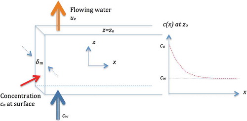
where c(x) is the concentration at z = z_o.

Two simple cases are treated. The first is when the water flow is caused by a regional hydraulic gradient. The second case is when the water flow is caused by the buoyancy generated by the in or out diffusion of salt that changes the density of the water.

III.B. Regional Hydraulic Gradient

In this case, as a first approximation, the flow velocity is taken to be constant everywhere in the slot. In addition to the regional gradient, especially for more transmissive fractures, it depends on the transmissivity of other surrounding fractures in the network. Low-transmissivity fractures may well limit the flow rate in a connected highly transmissive fracture.

Equation (2) simplifies to

(3) $N={\delta }_m{u}_z\underset{0}{\overset{\mathrm{\infty }}{\int }}\left(c\left(x\right)-c_w\right)dx.$(3)

The concentration profile perpendicular to the interface along the fracture can be described by Eq. (4) (5):

(4) $c\left(x\right)-c_w=(c_o-c_w)\mathrm{e}\mathrm{r}\mathrm{f}\mathrm{c}\left(\frac{x}{2\sqrt{D_w{t}_w}}\right),$(4)

where erfc is the complementary error function. The residence time for the water to reach $z$ is

(5) $t_{w,z}=\frac{z}{u_z}.$(5)

At the downstream end $z_o$ the residence time is $t_w=\frac{{\displaystyle z_o}}{{\displaystyle u_z}}$.

At $z_o$, the integration of Eq. (4) gives the flow rate of solute:

(6) $N=(c_o-c_w)\frac{2}{\sqrt{\pi }}{\delta }_m{u}_z\sqrt{D_w{t}_w}=\mathrm{\Delta }c\frac{2}{\sqrt{\pi }}{\delta }_m\sqrt{D_w{z}_o{u}_z}.$(6)

The driving force for the mass transfer is $\mathrm{\Delta }c=(c_o-c_w)$.

This was recently confirmed by experiments also for a variable aperture slot.⁶

The penetration depth of solute is defined as the distance where the concentration of the solute into the water is 1% of $(c_o-c_w)$ and is obtained from Eq. (4):

(7) ${\eta }_{0.01}=3.64\sqrt{D_w{t}_w}.$(7)

For Eq. (7) to be valid, ${\eta }_{0.01}\gg {\delta }_m$. Otherwise, the friction at the buffer interface cannot be neglected.

In practice, in fractures in the bedrock the aperture ${\delta }_m$ cannot be measured, but the transmissivity of the slot T can. The flow is driven by the hydraulic gradient $\frac{{\displaystyle dh}}{{\displaystyle dz}}$, where h is the hydraulic head. This can also be assessed by measurement or by hydraulic modeling. The velocity is related to these entities by

(8) $u_z=\frac{T}{{\delta }_m}\frac{dh}{dz}.$(8)

Introducing Eq. (8) into Eq. (6) gives

(9) $N=\mathrm{\Delta }c\frac{2}{\sqrt{\pi }}\sqrt{D_w{z}_{o}T{\delta }_m\frac{dh}{dz}}.$(9)

Note that we so far have not used any potential relation between aperture and transmissivity.

IV. BUOYANCY-INDUCED FLOW

IV.A. Development of Simple Approximate Expression for Buoyancy-Driven Flow

When solute concentration influences the density of the water near the buffer this sets the water in motion, up or down, depending on if the water at the surface becomes less or more dense. Then the integral in Eq. (2), $\underset{0}{\overset{\mathrm{\infty }}{\int }}{u}_z\left(x\right)(c_o\left(x\right)-c_w)dx$, must account for simultaneous variations in velocity and concentration. They influence each other and that mutual effect must be derived.

Assuming that the concentration profile in the density-driven case can be approximated by the same expression as for the constant velocity case and that the relation between water density and solute concentration is linear, $\mathrm{\Delta }\rho =\alpha \left(c_o-c_w\right)$, a vertical hydraulic gradient $\frac{{\displaystyle \mathrm{\Delta }\rho \left(x=0\right)}}{{\displaystyle \rho }}$ = $\frac{{\displaystyle dh}}{{\displaystyle dz}}$ will result at the boundary between the water and the buffer. Equation (9) then may be used as an approximation. The error caused by using Eq. (4) is assessed in Sec. IV.B by comparison with a more accurate solution.

It should be noted that density-driven flow can be induced also in sloping fractures isolated from or connected to a network that does not allow much of the regional gradient to generate flow through it. Then internal circulation in the fracture still can develop and generate mass transfer to or from a deposition hole or a vault repository.

In Sec. IV.B, a fracture is modeled that is so tall that it can be approximated to be infinite and that circulation does not have to be considered. It suffices to consider only the region nearest to the buffer/water interface. This approximation can be used when the solute penetration depth ${\eta }_{0.01}\ll$ z_o, the length (height) of the interface and of the horizontal extent of the fracture.

IV.B. A More Accurate Solution of the Governing Equations

Equations (10) through (14) govern the flow and salt transport in a vertical narrow two-dimensional slot⁵:

(10) $\frac{\mathrm{\partial }{u}_x}{\mathrm{\partial }x}+\frac{\mathrm{\partial }{u}_z}{\mathrm{\partial }z}=0,$(10)

(11) $u_x=-\frac{k}{\mu }\frac{\mathrm{\partial }p}{\mathrm{\partial }x},$(11)

(12) $u_z=-\frac{k}{\mu }\left(\frac{\mathrm{\partial }p}{\mathrm{\partial }z}+\rho g\right),$(12)

(13) $\frac{\mathrm{\partial }c}{\mathrm{\partial }t}=-u_x\frac{\mathrm{\partial }c}{\mathrm{\partial }x}-u_z\frac{\mathrm{\partial }c}{\mathrm{\partial }z}+D_w\left(\frac{{\mathrm{\partial }}^{2}c}{\mathrm{\partial }{x}^2}+\frac{{\mathrm{\partial }}^{2}c}{\mathrm{\partial }{z}^2}\right),$(13)

and

(14) $\rho ={\rho }_o\left(1+\alpha c\right),$(14)

where

$k$ =	=	permeability
$p$ =	=	pressure
$\mu$ =	=	water viscosity
$\rho$ =	=	density
g =	=	gravitation constant.

The considered region extends from x = 0 to $\mathrm{\infty }$ and from z = −$\mathrm{\infty }$ to $\mathrm{\infty }$. On the boundary at x = 0, the concentration c = c_o for z > 0 and the far-away water has concentration c_w.

For the problem at hand when only buoyancy-generated flow acts, it is assumed that the velocity and concentration profiles have reached a steady state. This can be attained for times much longer than the water to reach z_o. Then $\frac{{\displaystyle \mathrm{\partial }c}}{{\displaystyle \mathrm{\partial }t}}$ can be neglected and the problem becomes time independent. An exact analytical solution to this problem has been derived by Ene and $\mathrm{P}\mathrm{o}\mathrm{l}\mathrm{i}\stackrel{⌣}{\mathrm{s}}\mathrm{e}\mathrm{v}\mathrm{s}\mathrm{k}\mathrm{i}$.⁷ From their results, Eq. (9) can be derived but gives 1.3 times smaller values for the constant $\frac{{\displaystyle 2}}{{\displaystyle \sqrt{\pi }}}$. The gradient $\frac{{\displaystyle dh}}{{\displaystyle dz}}$ is then defined by $\frac{{\displaystyle \mathrm{\Delta }\rho \left(x=0\right)}}{{\displaystyle \rho }}$. Also, the penetration depth ${\eta }_{0.01}$ is somewhat different with a constant 6.31 instead of 3.64 in Eq. (7). The shape of the concentration profile is also different.

Equations (6), (8), and (9) apply for flow through a porous medium in contact with the buffer. Then ${\delta }_m={\delta }_{zone}\epsilon$, where ${\delta }_{zone}$ is the thickness of the zone and $\epsilon$ is its porosity.

Ene and $\mathrm{P}\mathrm{o}\mathrm{l}\mathrm{i}\stackrel{⌣}{\mathrm{s}}\mathrm{e}\mathrm{v}\mathrm{s}\mathrm{k}\mathrm{i}$⁷ also treat the case when c_o varies along the wall.

The concept of the equivalent flow rate mentioned in Sec. I can be used in an illustrative way to describe the release and transport capacity of the water flowing past, e.g., a deposition hole for a canister with nuclear waste such as in the KBS-type repository. It is the solute release rate N divided by the driving force¹: $Q_{eq}=N/\mathrm{\Delta }c$. It has been useful when integrating radionuclide release and transport modeling with models that simulate water flow through and past repositories with a multitude of sources.

To apply these results, information on repository conditions is needed on density differences $\mathrm{\Delta }\rho$, transmissivities T, and apertures ${\delta }_m$ of the real fractures. This is treated in Secs. V and VI.

V. DENSITIES OF CLAY AND CONCRETE PORE WATER AND GROUNDWATER

Two materials that are used to enclose the radioactive waste are bentonite clays and concrete. Both materials are porous and the pore waters contain salts that can diffuse out or into the groundwater depending on where the concentration is largest. Only an outline of potential concentrations is presented in order to quantify the expected range of density differences. This will later be used in an illustrative example. As a first approximation, the density difference can be set to $\mathrm{\Delta }\rho \cong \mathrm{\Delta }c$ when c has unit of kilograms/cubic meters [Eq. (14)].

V.A. Groundwater

The salt content of groundwater varies with location, depth, and time. At Forsmark, the site selected for the Swedish repository for spent fuel, the intermediate depth groundwater (200 to 600 m) at present has a salinity between 2 and 10 kg/m³, as described in the Forsmark site description.⁸ Deep groundwaters (>600 m) can have more than 10 kg/m³ and shallow water has mostly less than 2 kg/m³. At larger depths, the salinity can be much higher than that in the oceans that have around 35 kg/m³.

V.B. Clay Pore Water

Bentonite pore water will be influenced by the dissolution of the minerals in the bentonite. Savage et al.^9,10 in their simulations predict salt concentrations from 1.4 g/L at pH 9, to 18 g/L at pH around 12. The components include calcium, sodium, magnesium, sulphate, carbonate, and other ions. As a first approximation this will increase the water density by 1.4 to 18 kg/m³.

V.C. Concrete Pore Water

Andersson et al.¹¹ pressed pore water from seven different concretes, mostly based on Portland cement with different additives. Sodium and potassium were the dominating cations with concentrations from 0.3 to 3.2 kg/m³ Na and 0.1 to 7.5 kg/m³ K. The pH varied between 12.4 and 13.5. Total salt concentrations were between 1.7 and 11.8 kg/m³.

V.D. The Range of Density Difference

The density differences between the pore water and groundwater can be expected not to exceed a few tens of kilograms/cubic meters and the density-induced gradient $\frac{{\displaystyle \mathrm{\Delta }\rho \left(x=0\right)}}{{\displaystyle \rho }}$ would not exceed a few percent at repository depth even when meteoric water invades over long times. This is an order of magnitude, or more, larger than typical hydraulic gradients at repository depth.⁸

VI. TRANSMISSIVITY AND FRACTURE APERTURE

VI.A. Transmissivity Determination

The transmissivity of fractures in rock in situ can be measured by several techniques in boreholes (see for example, Ripatti et al.¹²). The principle is to induce a hydraulic head difference between the borehole and the far-away water in the fractured rock. From the measured flow rate to or from each location with an identified fracture and the head difference, the transmissivity T of the fractures can be determined.

VI.B. Fracture Aperture

The magnitude of the fracture aperture is central to the problem described in this paper and therefore will be discussed first. Fracture apertures cannot be measured in situ. From transmissivity data, estimates of the aperture can be made by the cubic law. This is valid for laminar flow in a parallel aperture slot with smooth walls but is not necessarily a proper measure of the mass balance aperture ${\delta }_m$. This is the aperture that describes the volume of mobile water per fracture area and could also account for the presence of infill and for fracture zones.

The cubic law aperture ${\delta }_c$ describes the relationship between transmissivity and aperture for an ideal slot with smooth walls when the flow is laminar:

(15) ${\delta }_c={\left(12T\frac{{\mu }_w}{{\rho }_{w}g}\right)}^{1/3}.$(15)

For individual fractures, ${\delta }_c$ can give a fair approximation of the mass balance aperture ${\delta }_m$ for real variable aperture fractures (Witherspoon et al.¹³). Obviously, this cannot be the case for fracture zones where the main resistance to flow is caused by the presence of particles filling in the fracture. This is better modeled as a slot with a porous medium with a given width and porosity. For the mass balance, the aperture will be the zone width times its porosity.

Attempts have been made to use in situ tracer experiments to determine ${\delta }_m$. Experimentally the mass balance aperture can be estimated from the fracture volume and the residence time $t_w$ for a flow rate through this volume. One often-used technique to do this is by in situ tracer tests. By pumping water out from a section in a borehole that intersects a fracture and measuring the residence time of the water by a tracer injected into the same fracture at a certain distance from the pumping hole, the aperture can be derived. Assuming that the fracture has reasonably similar properties everywhere, the volume of the water is taken to be the aperture times the area of a circle with the radius equal to the distance between injection and pumping hole. This determines the residence time of the flow rate. As the distance between the boreholes, r is very much larger than the radii of the boreholes the mass balance aperture is obtained from:

(16) ${\delta }_m=\frac{Q_w}{\pi r^2},$(16)

where Q is the pumping flow rate. For this technique to be valid it is essential that all flow rate to the pumping location passes the intended fracture and that the measured residence time is representative of the entire fracture. If there is maldistribution of flow by so-called channeling and the tracer is injected in the fast channel, which makes up a fraction $\beta$ of the entire fracture, ${\delta }_m$ can be overestimated by a fraction 1/$\beta .$ Considering that the pumping location will probably be chosen in a fracture where a high transmissivity location is intersected, $\beta$ is probably small. If the injection is made in a slow channel, the residence time could be dominated by the time for this flow to reach either the pumping hole or to intersect the fast channel somewhere. This aggravates the problem considerably. Also if the fracture has been fed by water from intersecting fractures in a leaking rock matrix, the Q in Eq. (16) is overestimated and the aperture would also be overestimated.

Hjerne et al.¹⁴ analyzed 74 in situ experiments from six different sites. They found that ${\delta }_m$ was about 100 times larger than ${\delta }_c$ over a range of fracture transmissivities from 10⁻⁹ to 10⁻³ m²/s. For the transmissivity 10⁻⁹ m²/s, which is a very tight fracture, the ${\delta }_m$ aperture is 0.4 mm. For a transmissivity of 10⁻⁶ m²/s, it is 4 mm. It may be noted that the 4-mm aperture open single fractures have not been observed in tunnels and drifts in crystalline rocks at repository depths.

Similar discrepancies between ${\delta }_m$ and ${\delta }_c$ were found in the so-called TRUE experiments (Neretnieks and Moreno¹⁵). At this site, transmissivities had been measured in boreholes surrounding the pumping and tracer injection boreholes. These showed that the target fracture, called feature A, must be intersected by many water-conducting fractures from which inflow contributed considerably to the pumping flow rate. Such information on fracture networks surrounding the target fracture is not available for the Hjerne et al.¹⁴ evaluations.

We conclude that the apertures, so far determined from tracer tests in crystalline rocks, do not seem to represent realistic values of mechanic apertures and that these can better be estimated by hydraulic tests.

VII. EXAMPLES

VII.A. Analytical Model

In this example, a vault with two vertical sides 20 m high is intersected by a vertical fracture. Figure 2 shows the equivalent flow rate for flow around both sides of a vault repository $Q_{eq}=2N/\mathrm{\Delta }c$ based on Eq. (9) as a function of fracture transmissivity for two different gradients and when using cubic law aperture ${\delta }_c$ for ${\delta }_m$. For gravity-driven flow, $Q_{eq}$ is 1.3 times lower as explained in Sec. IV.B.

Fig. 2. $Q_{eq}$ as a function of fracture transmissivity for two different hydraulic gradients.

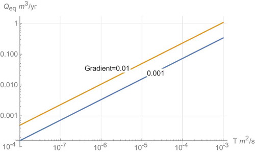
Figure 2 illustrates the main results and influences. It gives $Q_{eq}$ as a function of the transmissivity of the fracture with the gradient as a parameter. The gradient of the gravity-driven flow depends only on the concentration/density difference between the pore water in the buffer and the far-away water in the fracture. It is seen from Eq. (9) that scaling to another mass balance aperture can be done simply. The solution depends on the central entities in the following way: $\sqrt{D_w{z}_{o}T{\delta }_m\frac{{\displaystyle dh}}{{\displaystyle dz}}}$.

A larger or smaller vertical extent z_o and the mass balance aperture scale by the square root of the magnitude of these entities. Should one, for example, believe that the mass balance aperture ${\delta }_m$ is 100 times larger than ${\delta }_c$, as indicated by Hjerne et al.,¹⁴ then the results change by a factor of 10.

Figure 3 shows the velocity $u_z$ as well as the penetration depth ${\eta }_{0.01}$, which illustrates the width of the mobilized water at the interface to the buffer.

Fig. 3. (a) Velocity and (b) penetration depth as a function of transmissivity for cubic law fractures.

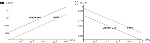
It is seen that the buoyancy-driven flow gives rise to a considerable velocity and that the width of the mobilized water ranges from a few centimeters to on the order of a meter.

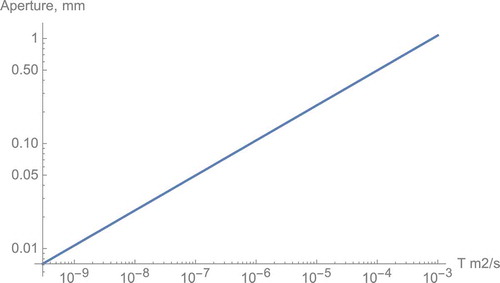
Figure 4 shows the fracture aperture ${\delta }_c$ versus the transmissivity T.

Fig. 4. Fracture aperture ${\delta }_c$ versus transmissivity T.

VII.B. Numerical Solutions

The analytical model has been verified by numerical calculations solving Eqs. (10) through (14) for the simple case of a vertical fracture open at the bottom and the top using COMSOL Multiphysics®.¹⁶ It was also found that a steady-state flow pattern was attained after a few water residence times of the water in the fracture.

We do not show results for larger transmissivities because fractures with transmissivities larger than 10⁻⁶ m²/s are likely to consist of multiple connected fractures and the cubic law between mechanic aperture and transmissivity is probably not valid. For larger transmissivities, it is better to make independent assessments of transmissivity and aperture than to use the cubic law.

VIII. FURTHER FATE OF THE BUOYANT STREAM

If the direction of the induced flow is upward, i.e., it contains less dense water than the surrounding water then it would “rapidly” reach the biosphere. If the water is denser, it would sink to a level where the salinity is similar to that in the stream and would then flow with that water driven by the hydraulic gradient in that location.

We illustrate the further fate of the buoyant stream with a case in which the stream has a lower density and therefore rises upward in the z-direction. The stream flows in surrounding water that has concentration c_o. Salt diffuses from the surrounding water into the stream. The concentration difference between the stream and surrounding water decreases and the rise velocity decreases. As the velocity decreases, diffusion is given more time to even out the concentration difference further, decreasing velocity, etc. Considering that it was shown in Fig. 3 that the stream velocity could be thousands of meters/year already for not very transmissive fractures it is of interest to explore the conditions under which equilibration of the stream can substantially slow down the velocity. Such a rising stream could otherwise rapidly rise also through a mildly downward moving groundwater flow driven by the regional hydraulic gradient.

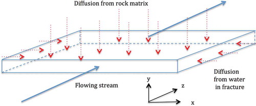
There are two ways the stream can take up more salt. One is from the surrounding water in the fracture and the other is from the pore water in the rock matrix. Figure 5 illustrates these sources.

Fig. 5. The flowing stream with low concentration takes up salt from water in the fracture and from the surrounding porous rock matrix with higher salt concentration.

VIII.A. Salt from Matrix Pore Water

We first explore the diffusion from the matrix. The stream will be fed by salt from the pore water in the rock matrix by what is called matrix diffusion, which can be a very important mechanism in narrow fractures with large fracture surface per seeping water flow rate for radionuclide retardation.

Diffusion of solute from the water in the fracture is already included in the mass balance [Eq. (13)]. To include the matrix diffusion Eq. (13) must be supplemented by a sink term and an additional partial differential equation describing the molecular diffusion in the rock matrix. Equation (13) with sink term, the rightmost term, becomes

(17) $\frac{\mathrm{\partial }c}{\mathrm{\partial }t}=-u_x\frac{\mathrm{\partial }c}{\mathrm{\partial }x}-u_z\frac{\mathrm{\partial }c}{\mathrm{\partial }z}+D_w\left(\frac{{\mathrm{\partial }}^{2}c}{\mathrm{\partial }{x}^2}+\frac{{\mathrm{\partial }}^{2}c}{\mathrm{\partial }{z}^2}\right)+{\left.\frac{2D_p\epsilon }{{\delta }_m}\frac{\mathrm{\partial }{c}_p}{\mathrm{\partial }y}\right|}_{y=0},$(17)

where

$D_p$=	=	pore diffusion coefficient
$\epsilon$ =	=	matrix porosity
$c_p$ =	=	salt concentration in the pore water
y =	=	distance into the rock matrix.

The diffusion equation in the matrix pore water is

(18) $R_d\frac{\mathrm{\partial }{c}_p}{\mathrm{\partial }t}=D_p\frac{{\mathrm{\partial }}^2{c}_p}{\mathrm{\partial }{y}^2},$(18)

where $R_d$ is the retardation factor of the solute in the rock matrix and it is unity for the nonsorbing salts we discuss here.

Matrix diffusion is an important process for radionuclide transport and retardation in fractured crystalline rock.¹⁷ It plays a central role in the models used to simulate radionuclide migration from repositories in fractured crystalline rock.^18,19 Equations (10), (11), (12), (14), (17), and (18) must be solved simultaneously. This three-dimensional problem must be solved by numerical methods. However, one can gain some insights and get an impression of when the exchange by matrix diffusion will and will not influence the concentration change, and thus, the density difference and thereby the vertical velocity u_z in more than a negligible manner.

In this approach, we first consider a case with constant velocity to see if the salt from the matrix could noticeably influence the concentration and thereby the velocity. u_z can be taken from Eq. (8) or Fig. 2 for different transmissivities. We then follow the one-dimensional vertically rising stream and assess how the salt diffuses in from the rock matrix in contact with this stream. For the diffusion of solute in the water-filled fracture, the terms $D_w\left(\frac{{\displaystyle {\mathrm{\partial }}^{2}c}}{{\displaystyle \mathrm{\partial }{x}^2}}+\frac{{\displaystyle {\mathrm{\partial }}^{2}c}}{{\displaystyle \mathrm{\partial }{z}^2}}\right)$ in Eq. (17) are neglected with the argument that advection strongly dominates over diffusion. Equation (17) then reduces to

(19) $\frac{\mathrm{\partial }c}{\mathrm{\partial }t}=-{\left.u_z\frac{\mathrm{\partial }c}{\mathrm{\partial }z}+\frac{2D_p\epsilon }{{\delta }_m}\frac{\mathrm{\partial }{c}_p}{\mathrm{\partial }y}\right|}_{y=0}.$(19)

With the initial condition that the rock matrix pore water has salt concentration $c_o$, the seeping water at the inlet, i.e., when just leaving the vault has a mean concentration of $c_w$ the solution to Eqs. (19) and (18) is¹⁷

(20) $\frac{c_o-c}{c_o-c_w}=\mathrm{e}\mathrm{r}\mathrm{f}\mathrm{c}\left(\frac{\sqrt{D_p}{\displaystyle \epsilon \frac{z_o}{u_z}}}{{\displaystyle {\delta }_m\sqrt{t-\frac{z_o}{u_z}}}}\right),$(20)

where z_o is the travel length alongside the fracture and t is the time since the stream entered the fracture. Figure 6 shows plots of the concentration evolution 200 m above the source based on Eq. (20) for three combinations of transmissivity and density-induced gradient. The cases were chosen such that matrix diffusion could be expected to have some impact on the equilibration of the rising stream, i.e., low transmissivity and low gradient. Figure 6 shows that a stream with concentration c_w that enters a “virgin” flow path in which the matrix pore water has concentration c_o will rapidly deplete the matrix pore water adjacent to the flow path and along the flow path and will decrease further uptake so that the effluent after 200 m has essentially the same concentration as at the inlet.

Fig. 6. Plots of the concentration evolution 200 m above the source based on Eq. (20) for three combinations of transmissivity and density-induced gradient.

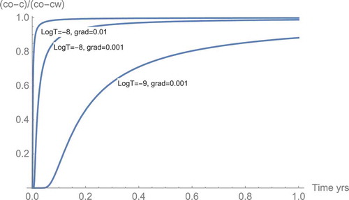
It is seen that for transmissivities as low as T = 10⁻⁸ m²/s, which is already a quite low transmissivity, the breakthrough curve of the salt is nearly instantaneous on the timescales of interest but that the concentration then rapidly approaches that at the inlet. This is because the matrix pore water is rapidly depleted and further transport from the matrix decreases rapidly. Only in a very tight fracture, T = 10⁻⁹ m²/s, will the matrix be able to supply sufficient salt to noticeably slow down the already very low velocity, less than a few meters/year (Fig. 3). This implies that the exchange with the matrix pore water has a negligible effect. Therefore, we conclude that the impact of matrix diffusion on the slowdown of the rising plume can be neglected for more transmissive fractures.

VIII.B. Salt from Surrounding Water in the Fracture

The analytical model has been verified by numerical calculations solving Eqs. (10) through (14) for the simple case of a vertical fracture open at the bottom and the top using COMSOL Multiphysics. This is shown in Table I. In the simulations it was also found that a steady-state flow pattern was attained after a few water residence times of the water in the fracture. As the stream flows upward it takes up salt from the surrounding water and from the pore water, which has the same concentration as the mobile water in the fracture. This uptake of salt decreases the buoyancy and the velocity slows down.

TABLE I Equivalent Flow Rates from Analytical Solution and Numerical Calculations Using D_w = 10⁻⁹ m²/s, ${\mu }_w$ = 0.001 Pa s, and $\frac{{\displaystyle \mathrm{\Delta }\rho }}{{\displaystyle \rho }}=0.001$, Height z_o = 20 m

T (m^2/s)	10^−8	10^−7	10^−6
Qeq (m^3/year)
Equation (9)	7.6 · 10^−5	3.5 · 10^−4	1.6 · 10^−3
Equation (9)/1.3	5.9 · 10^−5	2.7 · 10^−4	1.2 · 10^−3
Numerical	5.9 · 10^−5	2.7 · 10^−4	1.4 · 10^−3
${\eta }_{0.01}$ (m)
Equation (7)	0.78	0.36	0.17
With f 6.31	1.35	0.63	0.29
Numeric	1.28	0.59	0.29

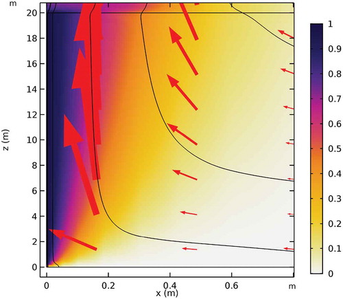
Figure 7a shows how the concentration distribution and the flow field for T = 10⁻⁸ m²/s and $\frac{\mathrm{\Delta }\rho }{\rho }=0.001$. Steady state had been reached after a few thousand years. The modeled region is a 220-m-high fracture with a 20-m-high source in the lower left corner. Figure 7b shows the results for a larger density difference,$\frac{\mathrm{\Delta }\rho }{\rho }=0.01$, which reached steady state after about 40 years. Figure 8 shows an enlargement of the source region of Fig. 7a.

Fig. 7. The flow field and concentration profile in a 220-m-high fracture with a 20-m-high source in the lower left corner for T = 10⁻⁸ and a density difference of (a) $\frac{{\displaystyle \mathrm{\Delta }\rho }}{{\displaystyle \rho }}=$ 0.001 and (b) $\frac{{\displaystyle \mathrm{\Delta }\rho }}{{\displaystyle \rho }}=$ 0.01. The color code shows the relative concentration difference.

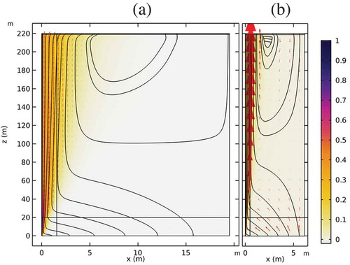
Fig. 8. Enlargement of the left corner of Fig. 7a showing the flow field and concentration profile near the 20-m-high source on the left side for T = 10⁻⁸ and a density difference of $\frac{{\displaystyle \mathrm{\Delta }\rho }}{{\displaystyle \rho }}=$ 0.001.

The penetration depths ${\eta }_{0.01}$ in Fig. 7a at 20 and 219 m are 1.28 and 9.38 m, respectively. The highest velocity at the same locations is 4.4 · 10⁻⁷ and 1.1 · 10⁻⁷ m/s. The residence time from 20 to 219 m, at x = 0, is 38.6 years.

The penetration depths ${\eta }_{0.01}$ in Fig. 7b at 20 and 219 m are 0.43 and 2.29 m, respectively. The highest velocity at the same locations is 4.4 · 10⁻⁶ and 1.3 · 10⁻⁶ m/s. The residence time from 20 to 219 m, at x = 0, is 3.7 years.

Figure 9 shows concentration and flux profiles at steady state for the same case at 20-, 120-, and 219-m height.

Fig. 9. (a) Concentration and (b) flux profiles at steady state at z = 20-, 120-, and 219-m height.

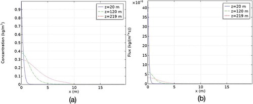
The stream has widened and slowed down considerably during its vertical passage 200 m above the source in this case.

For comparison, for a case with T = 10⁻⁶ m²/s, the penetration depths ${\eta }_{0.01}$ at 20 and 219 m are 0.29 and 1.66 m, respectively, The highest velocity at the same locations is 9.2 · 10⁻⁶ and 2.6 · 10⁻⁶ m/s. The residence time from 20 to 219 m, at x = 0, is 1.7 years. For the higher transmissivity, the stream moves very quickly and is hardly slowed down by the dilution.

IX. DISCUSSION AND CONCLUSIONS

The buoyancy can also be caused by temperature differences generated by heat-producing nuclear waste such as spent nuclear fuel which can heat the buffer material by several tens of degrees Celsius, over long times. The same equations can be used as elaborated by Holzbecher.²⁰ However, because thermal diffusivity is about two orders of magnitude larger than solute diffusivity, the stream would more rapidly equilibrate and slow down. Also, conduction from the rock matrix would become effective.

The buoyancy-driven mass transfer and that which is induced by a hydraulic gradient are very similar. The former results in 30% smaller transfer rates when compared for the same hydraulic gradient. The factor in the analytical solution was confirmed by the numerical solution, showing that the very simple analytical solution can be used to assess Q_eq. The buoyancy-induced gradient can be expected to be on the order of a few percent and less. The density-driven flow will decrease with time as the concentration difference between the buffer and the flowing water decreases over time.

The decrease rate can be illustrated in the following way. The pore water in a part of the buffer in the vault straddling the fracture is always well mixed due to molecular diffusion. This is a reasonable approximation considering that the characteristic for diffusion is small compared to the times of interest. If the water volume in the buffer that can be equilibrated is V_w and the equivalent flow rate is Q_eq, the concentration difference $\mathrm{\Delta }c$ between buffer water and flowing water changes in time as

(21) $\mathrm{\Delta }c\left(t\right)=\mathrm{\Delta }c\left(t=0\right)\times \mathrm{E}\mathrm{x}\mathrm{p}\left(\frac{-Q_{eq}}{V_w}t\right).$(21)

For large vault repositories this phenomenon will be more pronounced, the taller the repository is. For illustration, consider a vault that is 20 m high and 20 m wide with 1-m-thick bentonite buffer between the walls and the waste. The vault is intersected by a fracture and water can flow on both vertical sides generating a Q_eq of 0.01 m³/year. The porosity of the bentonite is 50%. On each side of the fracture along the vault, a 1-m-long bentonite section is accessible by diffusion to the fracture intersection. The water in the pore volume of the bentonite that can exchange solute with the flowing water on both sides of the vault is $({20}^2-{18}^2)\times 2\times 0.5=76{\mathrm{m}}^3$. This gives a fraction $\frac{{\displaystyle Q_{eq}}}{{\displaystyle V_w}}=$ 1.3 $\times$ 10⁻⁴ year⁻¹ of the solute concentration difference that will be exchanged per year. The buoyancy-induced flow can last for a long time under these conditions and impact the release exchange rate of solutes between vault and groundwater. However, it still remains to be addressed how the density differences can be determined, how they change over time, and if there are additional mechanisms that generate buoyancy effects.

There is a large difference between the cubic law–derived data and those presented by Hjerne et al.,¹⁴ about a factor of 100. At present, it seems likely that the actual mass balance aperture is closer to the cubic law aperture for individual fractures. The tracer-derived aperture data may not be meaningful for either individual fractures or for fracture zones.

Acknowledgments

The financial support from the Swedish Nuclear Fuel and Waste Management Co, SKB, is gratefully acknowledged. We also thank Luis Moreno for his advice.

References

- I. NERETNIEKS, “Transport Mechanisms and Rates of Transport of Nuclides in the Geosphere as Related to the Swedish KBS Concept,” Proc. Int. Atomic Energy Agency IAEA–SM–243/108, Vienna, Austria, July 2–6, 1979, pp. 315.
- P. L. CHAMBRÉ et al., “Analytical Performance Models for Geologic Repositories,” LBL-UCB-NE-4017, UC70, Earth Sciences Division, Lawrence Berkeley Laboratory and Department of Nuclear Engineering, University of California, Berkeley (1982).
- L. LIU and I. NERETNIEKS, “Analysis of Fluid Flow and Solute Transport in a Fracture Intersecting a Canister with Variable Aperture Fractures and Arbitrary Intersection Angles,” Nucl. Technol., 150, 132 (2005); https://doi.org/10.13182/NT05-A3611.
- I. NERETNIEKS, L. LIU, and L. MORENO, “Mass Transfer Between Waste Canister and Water Seeping in Rock Fractures Revisiting the Q-Equivalent Model,” SKB Technical Report, TR-10-42, Svensk Kärnbränslehantering AB (2010).
- R. B. BIRD, W. E. STEWART, and E. N. LIGHTFOOT, Transport Phenomena, 2nd ed., Wiley (2002).
- H. WINBERG-WANG, “Diffusion in a Variable Aperture Slot: Impact on Radionuclide Release from a Repository for Spent Fuel,” Nucl. Technol., 204, 184 (2018); https://doi.org/10.1080/00295450.2018.1469348.
- H. I. ENE and D. POLI⌣SEVSKI, Thermal Flow in Porous Media, p. 194, Reidel Publ. Comp., Dordrecht (1987).
- “Site Description Forsmark,” SKB Technical Report, TR-08-05, Svensk Kärnbränslehantering AB (2008); http://www.skb.com/publication/1868223/TR-08-05.pdf (current as of May 10, 2018).
- D. SAVAGE et al., “Testing Geochemical Models of Bentonite Pore Water Evolution Against Laboratory Experimental Data,” Phys. Chem. Earth, 36, 1817 (2011); https://doi.org/10.1016/j.pce.2011.07.025.
- D. SAVAGE et al., “An Evaluation of Models of Bentonite Pore Water Evolution,” SSM Report 2010:12 (2010); https://www.stralsakerhetsmyndigheten.se/en/publications/reports/waste-shipments-physical-protection/2010/201012/ (current as of May 10, 2018).
- K. ANDERSSON et al., “Chemical Composition of Cement Pore Waters,” Cem. Concr. Res., 19, 327 (1989); https://doi.org/10.1016/0008-8846(89)90022-7.
- K. RIPATTI, J. KOMULAINEN, and J. J. PÖLLÄNEN, “Difference Flow and Electrical Conductivity Measurements at the Olkiluoto Site in Eurajoki, Drillholes OL-KR56, OL-KR57 and OL-KR57B,” Posiva Working Report, 2013-26 (2013); http://posiva.fi/en/databank/workreports/difference_flow_and_electrical_conductivity_measurements_at_the_olkiluoto_site_in_eurajoki_drillholes_ol-kr56_ol-kr57_and_ol-kr57b.1874.xhtml?xm_col_report_year=2013&xm_col_type=5&cd_order=col_report_number&cd_offset=40#.W401pJMzbVo (current as of May 10, 2018).
- P. A. WITHERSPOON et al., “Validity of Cubic Law for Fluid Flow in Deformable Rock Fracture,” Water Resour. Res., 16, 1016 (1980); https://doi.org/10.1029/WR016i006p01016.
- C. HJERNE, R. NORDQVIST, and J. HARRSTRÖM, “Compilation and Analyses of Results from Cross-Hole Tracer Tests with Conservative Tracers,” SKB Report, R-09-28, Svensk Kärnbränslehantering AB (2010).
- I. NERETNIEKS and L. MORENO, “Prediction of Some in Situ Tracer Tests with Sorbing Tracers Using Independent Data,” J. Contam. Hydrol., 61, 351 (2003); https://doi.org/10.1016/S0169-7722(02)00123-7.
- COMSOL website; https://www.comsol.com/model/buoyancy-flow-with-darcy-s-law-8212-the-elder-problem-657 (current as of Oct. 15, 2018).
- I. NERETNIEKS, “Diffusion in the Rock Matrix: An Important Factor in Radionuclide Retardation?” J. Geophys. Res., 85, 4379 (1980); https://doi.org/10.1029/JB085iB08p04379.
- “Long-Term Safety for the Final Repository for Spent Nuclear Fuel at Forsmark Main Report of the SR-Site Project,” SKB Technical Report, TR-11-01, Svensk Kärnbränslehantering AB (2011).
- “Safety Case for the Disposal of Spent Nuclear Fuel at Olkiluoto—Performance Assessment 2012,” Posiva Oy., Posiva Report Number 2012-04 (2012); ISBN 978-951-652-187-2.
- E. HALZBECHER, Modeling Density-Driven Flow in Porous Media, 1st ed., Springer-Verlag, Heidelberg, Germany (1998).