Sockeye: A One-Dimensional, Two-Phase, Compressible Flow Heat Pipe Application

Abstract

Sockeye is a heat pipe analysis application based on the Multiphysics Object-Oriented Simulation Environment (MOOSE) finite element framework. The primary purpose of Sockeye is to provide a transient heat pipe simulation tool to be used in the analysis of nuclear microreactor designs. Sockeye provides the capability to perform one-dimensional, two-phase, compressible flow simulation of a heat pipe working fluid and two-dimensional, axisymmetric heat conduction for the heat pipe cladding and its surroundings. Sockeye is demonstrated against analytical solutions and experimental data from the SAFE-30 heat pipe module test.

Keywords:

• MOOSE
• sockeye
• heat pipe

I. INTRODUCTION

Heat pipes are very efficient heat transfer devices in terms of their effective thermal conductivity, their cross-sectional area, and their ability to transport heat over great distances. Additionally, their construction and operation are simple, requiring no moving parts or external control mechanisms, and they demonstrate a high reliability. All of these qualities make heat pipes a very attractive heat transfer option for a wide variety of applications such as space applications, refrigeration, air conditioning, oil pipelines, snow melting and deicing, and electronic cooling.^1,2

One of these applications is the passive heat removal in advanced nuclear reactor concepts. The latest generation of proposed nuclear reactors features many designs that fall under the category of small modular reactors (SMRs), and many of these designs utilize heat pipes to achieve compact heat exchangers. SMRs are attractive for a number of reasons. The modular nature allows units to be factory built and shipped to the site, reducing construction time and cost, and more units can be added as power demand increases. The small, modular approach also leads to a much smaller initial capital investment than traditional, large-scale power plants. The small scale of these reactors allows for flexibility in site location; these reactors can be operated in remote areas and can be transported relatively quickly to provide emergency power for sites of natural disasters.

The Nuclear Energy Advanced Modeling and Simulation program is developing tools for modeling advanced reactors such as SMRs, and the program’s heat pipe application, currently under development, is called Sockeye and is the focus of this work. Sockeye is based on the Multiphysics Object-Oriented Simulation Environment (MOOSE) finite element framework.³ A diverse range of applications have been built using the MOOSE framework, and the ability to couple different physics is a core capability the framework provides. A microreactor multiphysics simulation, for example, can include domains such as thermal hydraulics, neutronics, and thermomechanics. Multiphysics coupling of Sockeye is not the focus of this work, however; see Ref. 4 for an example of Sockeye coupling.

Heat pipes, while very reliable in their respective operating ranges, must be operated with care because their heat transport capability can be limited by a number of different effects. Some degree of analysis can be performed analytically, but transient simulation allows these limits to be investigated with greater extent and confidence. Steady-state analyses of operational limits can be valuable tools for heat pipe design and analysis, but they have serious shortcomings when employed for transient studies. They do not consider the transient conditions imposed on a heat pipe, and they fail to answer questions regarding the transient response of heat pipes. For instance, questions such as heat transfer rate, how fast a heat pipe fails, and whether a heat pipe can recover are important questions that transient simulation can answer.

There are a number of different approaches to modeling transient heat pipe behavior, each with its own advantages and disadvantages. Lumped capacitance models do not feature a formal spatial discretization but instead consider heat transfer between a (small) number of volumes. These models have a huge advantage in terms of run time and development time and in many cases make accurate predictions of heat pipe transient behavior. Faghri and Harley⁵ created a lumped model that could be used for both conventional and gas-loaded heat pipes. Reid⁶ presented Heat Pipe Approximation (HPAPPX), which divided the heat pipe into an evaporator region and four condenser regions and used analytic operational limit relations to limit heat flow from the evaporator. This model was applied to the sodium heat pipe module test for the SAFE-30 reactor prototype⁷ and demonstrated good agreement with experimental thermocouple measurements. Reid notes that this model is able to capture basic transient response but is not suitable for rapid transients. Another classification of heat pipe modeling approaches is that of thermal network analysis. This approach draws analogy between thermal systems and electrical circuits by relating temperatures to voltages and heat rate to current.² A number of efforts have been made for this approach, including Refs. 8910 through 11. Like the lumped models, these models can produce accurate predictions of transient thermal response but are unsuitable for transients in which fluid dynamics are of great importance. Another classification of heat pipe modeling is that of the effective heat conduction approach, where the entire heat pipe is modeled with heat conduction equations but choose thermal properties to effectively represent the heat transport capability of the heat pipe: The vapor core region is modeled using a very high thermal conductivity in accordance with the heat transport rate of the vapor flow and latent heat.^12,13 This is a very popular approach because its development is relatively simple, it offers spatial discretization, and when a heat pipe is fully started and operating well within limits, this approach can produce an accurate thermal response. Sockeye contains such a model, but its flow model is the focus of this work.

The most comprehensive models of heat pipe transient behavior are those that simulate the fluid dynamics of the heat pipe working fluid; however, these are also by far the most computationally expensive as they entail spatial discretization in one, two, or three dimensions. There are a variety of approaches to modeling the heat pipe working fluid. Bowman and Hitchcock¹⁴ modeled two-dimensional (2-D) compressible vapor flow for a simulated heat pipe, in which the circulation of a heat pipe vapor is approximated by blowing and sucking air through the porous walls of a pipe. Similarly, Cao and Faghri¹⁵ modeled 2-D compressible vapor flow of a heat pipe core, but they additionally coupled this to 2-D heat conduction in the heat pipe wick and wall and argued for the importance of modeling the heat pipe as a coupled system. Ransom and Chow¹⁶ presented ATHENA, which was an extension of RELAP5, to heat pipe analysis. Vapor and liquid phases are modeled in one dimension and are assumed to be separated. Void fraction was related to capillary pressure with an explicit time discretization, which Hall and Doster¹⁷ note led to severe time-step size restrictions for stability. Hall and Doster¹⁷ developed Thermal Hydraulic Response of Heat Pipes Under Transients (THROHPUT), a one-dimensional (1-D) code that accounts for all three phases (solid, liquid, vapor) of the working fluid and a noncondensable gas, as well as coupling to heat conduction in the wall. Tournier and El-Genk developed the Heat Pipe Transient Analysis Model¹⁸ (HPTAM), which considers the core, wick/annulus, and wall regions in two dimensions, coupled by appropriate interface conditions. In the HPTAM, the wick/annulus region is modeled by the Brinkman-Forchheimer extended Darcy flow model, and liquid pooling is modeled by having the vapor flow sweep off excess liquid (i.e., having a convex meniscus at pore sites) toward the condenser end. Cao and Faghri¹⁹ modeled startup in two dimensions by coupling a self-diffusion model for rarefied gas to the compressible Navier-Stokes equations for continuum vapor flow.

The goal of Sockeye is to provide a practical engineering tool to model heat pipes used in nuclear microreactors. The required scope of Sockeye includes the transient modeling of heat pipe operating limits, which excludes the use of lumped models, thermal network models, and effective heat conduction models. Thus simulation of fluid dynamics of the working fluid is necessary; however, the requirement of Sockeye to be a practical engineering tool excludes the use of 2-D and three-dimensional models due to computational expense, so a 1-D model is adopted. The most relevant reference point for this modeling approach is that of Hall and Doster’s code THROHPUT (Ref. 17), which features a number of modeling abilities not yet featured in Sockeye, including startup and noncondensable gases; however, Sockeye offers a number of potential advantages, such as the use of a well-posed two-phase model and the ability for pressure nonequilibrium.

This paper is organized as follows: Sec. II presents the models used in Sockeye, Sec. III gives an overview of the spatial and temporal discretization of the partial differential equations, Sec. IV describes plans for verification and validation, Sec. V gives some numerical demonstrations, and Sec. VI gives conclusions.

II. MODELS

Section II.A describes the models used for the 1-D, two-phase fluid flow of the heat pipe working fluid, and Sec. II.B describes the 2-D heat conduction in the heat pipe cladding and surroundings.

II.A. Two-Phase Flow

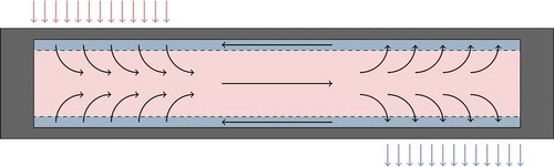
Heat pipes operate by taking advantage of the large amount of internal thermal energy that can be stored as latent heat. In the “evaporator” axial region of a conventional axial heat pipe, heat is supplied until the liquid working fluid vaporizes into the central core region, where the vapor flows to the other end of the heat pipe, termed the “condenser” region, where the fluid condenses and releases its latent heat. The liquid working fluid then returns to the evaporator end of the heat pipe, where the cycle continues. This is illustrated in Fig. 1. Note that there need not be a single evaporator or condenser region; these regions are determined by the conditions imposed on the heat pipe, not by manufacturing.

Fig. 1. Illustration of normal operation in a conventional axial heat pipe. Vapor is shown in pink, liquid in blue, and cladding in gray

Sockeye focuses on heat pipes of the “conventional” axial type, which consists of a long, straight tube (cladding) sealed at both ends containing a wick structure and a single, central vapor region. Sockeye models configurations that use a porous wick structure; it does not model grooved or arterial heat pipes. The porous wick structure is assumed to be uniform with a porosity $\phi$, permeability $K$, and pore radius $R_{\mathrm{p}\mathrm{o}\mathrm{r}\mathrm{e}}$. The wick may or may not be offset from the inner clad surface by a gap; this configuration is shown in Fig. 2, along with the relevant user-supplied radial dimensions. Note that the phase distribution in Fig. 2 is only a representation of the typical distribution under normal operating conditions; the liquid-vapor interface in Sockeye is not fixed at the inner surface of the wick but varies dynamically with the solution.

Fig. 2. Cross section of a heat pipe that may be modeled using Sockeye

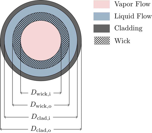
In the equations that follow, the cross-sectional area open to flow is denoted by $A$ and is computed from the dimensions given in Fig. 2 and the wick porosity:

(1) $A=A_{\mathrm{c}\mathrm{o}\mathrm{r}\mathrm{e}}+\phi A_{\mathrm{w}\mathrm{i}\mathrm{c}\mathrm{k}}+A_{\mathrm{a}\mathrm{n}\mathrm{n}},$(1)

where

$A_{\mathrm{c}\mathrm{o}\mathrm{r}\mathrm{e}}$ =	=	core cross-sectional area
$A_{\mathrm{w}\mathrm{i}\mathrm{c}\mathrm{k}}$ =	=	total wick cross-sectional area
$A_{\mathrm{a}\mathrm{n}\mathrm{n}}$ =	=	annulus cross-sectional area:

(2) $A_{\mathrm{c}\mathrm{o}\mathrm{r}\mathrm{e}}=\frac{\pi }{4}{D}_{\mathrm{w}\mathrm{i}\mathrm{c}\mathrm{k},\mathrm{i}}^2,$(2)

(3) $A_{\mathrm{w}\mathrm{i}\mathrm{c}\mathrm{k}}=\frac{\pi }{4}(D_{\mathrm{w}\mathrm{i}\mathrm{c}\mathrm{k},\mathrm{o}}^2-D_{\mathrm{w}\mathrm{i}\mathrm{c}\mathrm{k},\mathrm{i}}^2),$(3)

and

(4) $A_{\mathrm{a}\mathrm{n}\mathrm{n}}=\frac{\pi }{4}(D_{\mathrm{c}\mathrm{l}\mathrm{a}\mathrm{d},\mathrm{i}}^2-D_{\mathrm{w}\mathrm{i}\mathrm{c}\mathrm{k},\mathrm{o}}^2),$(4)

where, as shown in Fig. 2,

$D_{\mathrm{c}\mathrm{l}\mathrm{a}\mathrm{d},\mathrm{i}}$ =	=	inner cladding diameter
$D_{\mathrm{w}\mathrm{i}\mathrm{c}\mathrm{k},\mathrm{o}}$ =	=	outer wick diameter
$D_{\mathrm{w}\mathrm{i}\mathrm{c}\mathrm{k},\mathrm{i}}$ =	=	inner wick diameter.

The governing equations of two-phase flow in Sockeye derive from the seven-equation model,^20–23 which is a well-posed, nonequilibrium, compressible, two-phase-flow model. A number of changes are made to adapt the seven-equation model used by RELAP-7 to heat pipe flow^24,25:

1. Boiling is neglected; only interface evaporation/condensation occurs.

2. Heat conduction is added for the liquid phase.

3. Liquid friction uses a Darcy’s law term instead of a friction factor.

4. Velocity relaxation is neglected due to countercurrent flow.

5. Pressure relaxation is modified to account for the capillary pressure.

The resulting system of partial differential equations is as follows, where the subscript $\mathrm{\ell }$ denotes the liquid phase and the subscript $v$ denotes the vapor phase:

(5) $\frac{\mathrm{\partial }{\alpha }_{\mathrm{\ell }}A}{\mathrm{\partial }t}+u_{\mathrm{i}\mathrm{n}\mathrm{t}}\frac{\mathrm{\partial }{\alpha }_{\mathrm{\ell }}}{\mathrm{\partial }x}A=\mathrm{\Theta }\left(p_{\mathrm{\ell }}+\mathrm{\Delta }{p}_{\mathrm{c}\mathrm{a}\mathrm{p}}-p_v\right)A-\frac{{\mathrm{\Gamma }}_{\mathrm{i}\mathrm{n}\mathrm{t}}{a}_{\mathrm{i}\mathrm{n}\mathrm{t}}A}{{\rho }_{\mathrm{i}\mathrm{n}\mathrm{t}}},$(5)

(6) $\frac{\mathrm{\partial }{\alpha }_{\mathrm{\ell }}{\rho }_{\mathrm{\ell }}A}{\mathrm{\partial }t}+\frac{\mathrm{\partial }{\alpha }_{\mathrm{\ell }}{\rho }_{\mathrm{\ell }}{u}_{\mathrm{\ell }}A}{\mathrm{\partial }x}=-{\mathrm{\Gamma }}_{\mathrm{i}\mathrm{n}\mathrm{t}}{a}_{\mathrm{i}\mathrm{n}\mathrm{t}}A,$(6)

(7) $\frac{\mathrm{\partial }{\alpha }_{\mathrm{\ell }}{\rho }_{\mathrm{\ell }}{u}_{\mathrm{\ell }}A}{\mathrm{\partial }t}+\frac{\mathrm{\partial }{\alpha }_{\mathrm{\ell }}\left({\rho }_{\mathrm{\ell }}{u}_{\mathrm{\ell }}^2+p_{\mathrm{\ell }}\right)A}{\mathrm{\partial }x}=p_{\mathrm{i}\mathrm{n}\mathrm{t}}\frac{\mathrm{\partial }{\alpha }_{\mathrm{\ell }}}{\mathrm{\partial }x}A-{\mathrm{\Gamma }}_{\mathrm{i}\mathrm{n}\mathrm{t}}{u}_{\mathrm{i}\mathrm{n}\mathrm{t}}{a}_{\mathrm{i}\mathrm{n}\mathrm{t}}A-\frac{{\mu }_{\mathrm{\ell }}{u}_{\mathrm{\ell }}}{K}{A}_{\mathrm{w}\mathrm{i}\mathrm{c}\mathrm{k},\mathrm{\ell }}+{\alpha }_{\mathrm{\ell }}{\rho }_{\mathrm{\ell }}{g}_{x}A,$(7)

(8) $\begin{array}{rl}& \frac{\mathrm{\partial }{\alpha }_{\mathrm{\ell }}{\rho }_{\mathrm{\ell }}{E}_{\mathrm{\ell }}A}{\mathrm{\partial }t}+\frac{\mathrm{\partial }{\alpha }_{\mathrm{\ell }}{u}_{\mathrm{\ell }}\left({\rho }_{\mathrm{\ell }}{E}_{\mathrm{\ell }}+p_{\mathrm{\ell }}\right)A}{\mathrm{\partial }x}=p_{\mathrm{i}\mathrm{n}\mathrm{t}}{u}_{\mathrm{i}\mathrm{n}\mathrm{t}}\frac{\mathrm{\partial }{\alpha }_{\mathrm{\ell }}}{\mathrm{\partial }x}A\\ & +\frac{\mathrm{\partial }}{\mathrm{\partial }x}\left({\alpha }_{\mathrm{\ell }}{k}_{\mathrm{\ell }}\frac{\mathrm{\partial }{T}_{\mathrm{\ell }}}{\mathrm{\partial }x}A\right)-{\bar{p}}_{\mathrm{i}\mathrm{n}\mathrm{t}}\mathrm{\Theta }\left(p_{\mathrm{\ell }}+\mathrm{\Delta }{p}_{\mathrm{c}\mathrm{a}\mathrm{p}}-p_v\right)A\\ & +{\alpha }_{\mathrm{\ell }}{\rho }_{\mathrm{\ell }}{g}_x{u}_{\mathrm{\ell }}A+q_{\mathrm{\ell }}^{\mathrm{w}\mathrm{a}\mathrm{l}\mathrm{l}}{P}_{\mathrm{w}\mathrm{a}\mathrm{l}\mathrm{l}}+q_{\mathrm{\ell }}^{\mathrm{i}\mathrm{n}\mathrm{t}}{a}_{\mathrm{i}\mathrm{n}\mathrm{t}}A-{\mathrm{\Gamma }}_{\mathrm{i}\mathrm{n}\mathrm{t}}{E}_{\mathrm{\ell }}^{\mathrm{i}\mathrm{n}\mathrm{t}}{a}_{\mathrm{i}\mathrm{n}\mathrm{t}}A,\end{array}$(8)

(9) $\frac{\mathrm{\partial }{\alpha }_v{\rho }_{v}A}{\mathrm{\partial }t}+\frac{\mathrm{\partial }{\alpha }_v{\rho }_v{u}_{v}A}{\mathrm{\partial }x}={\mathrm{\Gamma }}_{\mathrm{i}\mathrm{n}\mathrm{t}}{a}_{\mathrm{i}\mathrm{n}\mathrm{t}}A,$(9)

(10) $\frac{\mathrm{\partial }{\alpha }_v{\rho }_v{u}_{v}A}{\mathrm{\partial }t}+\frac{\mathrm{\partial }{\alpha }_v\left({\rho }_v{u}_v^2+p_v\right)A}{\mathrm{\partial }x}=p_{\mathrm{i}\mathrm{n}\mathrm{t}}\frac{\mathrm{\partial }{\alpha }_v}{\mathrm{\partial }x}A+{\mathrm{\Gamma }}_{\mathrm{i}\mathrm{n}\mathrm{t}}{u}_{\mathrm{i}\mathrm{n}\mathrm{t}}{a}_{\mathrm{i}\mathrm{n}\mathrm{t}}A-\frac{1}{2}\frac{f_v{\alpha }_v{\rho }_v|u_v|u_v}{D_{\mathrm{w}\mathrm{i}\mathrm{c}\mathrm{k},\mathrm{i}}}A+{\alpha }_v{\rho }_v{g}_{x}A,$(10)

and

(11) $\begin{array}{rl}& \frac{\mathrm{\partial }{\alpha }_v{\rho }_v{E}_{v}A}{\mathrm{\partial }t}+\frac{\mathrm{\partial }{\alpha }_v{u}_v\left({\rho }_v{E}_v+p_v\right)A}{\mathrm{\partial }x}=p_{\mathrm{i}\mathrm{n}\mathrm{t}}{u}_{\mathrm{i}\mathrm{n}\mathrm{t}}\frac{\mathrm{\partial }{\alpha }_v}{\mathrm{\partial }x}A\\ & +{\bar{p}}_{\mathrm{i}\mathrm{n}\mathrm{t}}\mathrm{\Theta }\left(p_{\mathrm{\ell }}+\mathrm{\Delta }{p}_{\mathrm{c}\mathrm{a}\mathrm{p}}-p_v\right)A+{\alpha }_v{\rho }_v{g}_x{u}_{v}A\\ & +q_v^{\mathrm{w}\mathrm{a}\mathrm{l}\mathrm{l}}{P}_{\mathrm{w}\mathrm{a}\mathrm{l}\mathrm{l}}+q_v^{\mathrm{i}\mathrm{n}\mathrm{t}}{a}_{\mathrm{i}\mathrm{n}\mathrm{t}}A+{\mathrm{\Gamma }}_{\mathrm{i}\mathrm{n}\mathrm{t}}{E}_v^{\mathrm{i}\mathrm{n}\mathrm{t}}{a}_{\mathrm{i}\mathrm{n}\mathrm{t}}A.\end{array}$(11)

To briefly summarize the derivation of these equations, a phase function ${\chi }_k(\mathbf{x},t)$ is defined:

(12) ${\chi }_k(\mathbf{x},t)=\left\{\begin{array}{cc}1& \mathrm{i}\mathrm{f}(\mathbf{x},t)\mathrm{c}\mathrm{o}\mathrm{r}\mathrm{r}\mathrm{e}\mathrm{s}\mathrm{p}\mathrm{o}\mathrm{n}\mathrm{d}\mathrm{s}\mathrm{t}\mathrm{o}\mathrm{p}\mathrm{h}\mathrm{a}\mathrm{s}\mathrm{e}k\\ 0& \mathrm{o}\mathrm{t}\mathrm{h}\mathrm{e}\mathrm{r}\mathrm{w}\mathrm{i}\mathrm{s}\mathrm{e}\end{array}\right.,$(12)

which obeys the evolution equation:

(13) $\frac{\mathrm{\partial }{\chi }_k}{\mathrm{\partial }t}+{\mathbf{u}}_{\mathrm{i}\mathrm{n}\mathrm{t}}\cdot \mathrm{\nabla }{\chi }_k=0,$(13)

where ${\mathbf{u}}_{\mathrm{i}\mathrm{n}\mathrm{t}}$ is the interfacial velocity.²⁶ Each phase is assumed to obey the single-phase Euler equations, which along with Eq. (13(13) $\frac{\mathrm{\partial }{\chi }_k}{\mathrm{\partial }t}+{\mathbf{u}}_{\mathrm{i}\mathrm{n}\mathrm{t}}\cdot \mathrm{\nabla }{\chi }_k=0,$(13) ), get multiplied by the phase function and integrated over the cross-sectional area $A(x)$. The volume fractions appearing in the resulting equations are defined as follows:

(14) ${\alpha }_k(x,t)=\frac{1}{A(x)}\underset{A(x)}{\int }{\chi }_k(\mathbf{x},t)\mathrm{d}A,$(14)

where $A(x)$ is the flow cross-sectional area at axial position $x$. Note this definition implies the following, since $\sum _k{\chi }_k(\mathbf{x},t)=1$ on the domain $A(x)$:

(15) ${\alpha }_{\mathrm{\ell }}+{\alpha }_v=1.$(15)

The phasic thermodynamic and transport properties appearing in Eqs. (5)(5) $\frac{\mathrm{\partial }{\alpha }_{\mathrm{\ell }}A}{\mathrm{\partial }t}+u_{\mathrm{i}\mathrm{n}\mathrm{t}}\frac{\mathrm{\partial }{\alpha }_{\mathrm{\ell }}}{\mathrm{\partial }x}A=\mathrm{\Theta }\left(p_{\mathrm{\ell }}+\mathrm{\Delta }{p}_{\mathrm{c}\mathrm{a}\mathrm{p}}-p_v\right)A-\frac{{\mathrm{\Gamma }}_{\mathrm{i}\mathrm{n}\mathrm{t}}{a}_{\mathrm{i}\mathrm{n}\mathrm{t}}A}{{\rho }_{\mathrm{i}\mathrm{n}\mathrm{t}}},$(5) through (11(11) $\begin{array}{rl}& \frac{\mathrm{\partial }{\alpha }_v{\rho }_v{E}_{v}A}{\mathrm{\partial }t}+\frac{\mathrm{\partial }{\alpha }_v{u}_v\left({\rho }_v{E}_v+p_v\right)A}{\mathrm{\partial }x}=p_{\mathrm{i}\mathrm{n}\mathrm{t}}{u}_{\mathrm{i}\mathrm{n}\mathrm{t}}\frac{\mathrm{\partial }{\alpha }_v}{\mathrm{\partial }x}A\\ & +{\bar{p}}_{\mathrm{i}\mathrm{n}\mathrm{t}}\mathrm{\Theta }\left(p_{\mathrm{\ell }}+\mathrm{\Delta }{p}_{\mathrm{c}\mathrm{a}\mathrm{p}}-p_v\right)A+{\alpha }_v{\rho }_v{g}_x{u}_{v}A\\ & +q_v^{\mathrm{w}\mathrm{a}\mathrm{l}\mathrm{l}}{P}_{\mathrm{w}\mathrm{a}\mathrm{l}\mathrm{l}}+q_v^{\mathrm{i}\mathrm{n}\mathrm{t}}{a}_{\mathrm{i}\mathrm{n}\mathrm{t}}A+{\mathrm{\Gamma }}_{\mathrm{i}\mathrm{n}\mathrm{t}}{E}_v^{\mathrm{i}\mathrm{n}\mathrm{t}}{a}_{\mathrm{i}\mathrm{n}\mathrm{t}}A.\end{array}$(11) ) are intrinsic; that is, they are with respect only to the given phase, not the mixture. Density is denoted by ${\rho }_k$, pressure by $p_k$, temperature by $T_k$, specific total energy by $E_k$, dynamic viscosity by ${\mu }_k$, and thermal conductivity by $k_k$. The thermodynamic state $({\rho }_k,e_k)$ is used as input to the equation of state to compute other properties, where $e_k$ is the specific internal energy,

(16) $e_k=E_k-\frac{1}{2}{u}_k^2,$(16)

and where $u_k$ is the velocity component in the axis direction. The equations of state are discussed in Sec. II.A.4.

The interfacial velocity and pressure are derived from local Riemann problem solutions^26,27:

(17) $u_{\mathrm{i}\mathrm{n}\mathrm{t}}=\frac{Z_{\mathrm{\ell }}{u}_{\mathrm{\ell }}+Z_v{u}_v}{Z_{\mathrm{\ell }}+Z_v}+\mathrm{s}\mathrm{g}\mathrm{n}\left(\frac{\mathrm{\partial }{\alpha }_{\mathrm{\ell }}}{\mathrm{\partial }x}\right)\frac{p_v-p_{\mathrm{\ell }}}{Z_{\mathrm{\ell }}+Z_v},$(17)

(18) $p_{\mathrm{i}\mathrm{n}\mathrm{t}}={\bar{p}}_{\mathrm{i}\mathrm{n}\mathrm{t}}+\frac{Z_{\mathrm{\ell }}{Z}_v}{Z_{\mathrm{\ell }}+Z_v}\mathrm{s}\mathrm{g}\mathrm{n}\left(\frac{\mathrm{\partial }{\alpha }_{\mathrm{\ell }}}{\mathrm{\partial }x}\right)\left(u_v-u_{\mathrm{\ell }}\right),$(18)

and

(19) ${\bar{p}}_{\mathrm{i}\mathrm{n}\mathrm{t}}=\frac{Z_{\mathrm{\ell }}{p}_v+Z_v{p}_{\mathrm{\ell }}}{Z_{\mathrm{\ell }}+Z_v},$(19)

where $Z_k={\rho }_k{c}_k$ is the acoustic impedance of phase $k$, with $c_k$ being the sound speed in phase $k$. The remaining interfacial thermodynamic quantities are computed as follows, as presented in Ref. 26:

(20) $T_{\mathrm{i}\mathrm{n}\mathrm{t}}=T_{\mathrm{s}\mathrm{a}\mathrm{t}}({\bar{p}}_{\mathrm{i}\mathrm{n}\mathrm{t}}),$(20)

(21) ${\rho }_{\mathrm{i}\mathrm{n}\mathrm{t}}={\rho }_{\mathrm{\ell }}({\bar{p}}_{\mathrm{i}\mathrm{n}\mathrm{t}},T_{\mathrm{i}\mathrm{n}\mathrm{t}}),$(21)

(22) $h_k^{\mathrm{i}\mathrm{n}\mathrm{t}}=h_k({\bar{p}}_{\mathrm{i}\mathrm{n}\mathrm{t}},T_{\mathrm{i}\mathrm{n}\mathrm{t}}),$(22)

and

(23) $E_k^{\mathrm{i}\mathrm{n}\mathrm{t}}=h_k^{\mathrm{i}\mathrm{n}\mathrm{t}}-\frac{p_{\mathrm{i}\mathrm{n}\mathrm{t}}}{{\rho }_{\mathrm{i}\mathrm{n}\mathrm{t}}}+\frac{1}{2}{u}_{\mathrm{i}\mathrm{n}\mathrm{t}}^2,$(23)

where $T_{\mathrm{s}\mathrm{a}\mathrm{t}}(p)$, ${\rho }_{\mathrm{\ell }}(p,T)$, and $h_k(p,T)$ represent calls to equations of state.

Both phases exchange heat with the phasic interface. The heat flux to phase $k$ from the interface is denoted by $q_k^{\mathrm{i}\mathrm{n}\mathrm{t}}$ and is defined as follows:

(24) $q_k^{\mathrm{i}\mathrm{n}\mathrm{t}}={\mathcal{H}}_k^{\mathrm{i}\mathrm{n}\mathrm{t}}(T_{\mathrm{i}\mathrm{n}\mathrm{t}}-T_k),$(24)

where ${\mathcal{H}}_k^{\mathrm{i}\mathrm{n}\mathrm{t}}$ is the interfacial heat transfer coefficient for phase $k$. Sockeye has not yet developed a closure for this quantity, so this value is currently provided by the user. The interfacial mass flux ${\mathrm{\Gamma }}_{\mathrm{i}\mathrm{n}\mathrm{t}}$, defined as the net mass flux from liquid to vapor, is defined by performing a steady-state energy balance at the interface:

(25) ${\mathrm{\Gamma }}_{\mathrm{i}\mathrm{n}\mathrm{t}}=\frac{-q_{\mathrm{\ell }}^{\mathrm{i}\mathrm{n}\mathrm{t}}-q_v^{\mathrm{i}\mathrm{n}\mathrm{t}}}{h_v^{\mathrm{i}\mathrm{n}\mathrm{t}}-h_{\mathrm{\ell }}^{\mathrm{i}\mathrm{n}\mathrm{t}}}.$(25)

The interfacial area density $a_{\mathrm{i}\mathrm{n}\mathrm{t}}$ appearing in the interfacial terms is described in Sec. II.A.3.

The first term on the right side of Eq. (5)(5) $\frac{\mathrm{\partial }{\alpha }_{\mathrm{\ell }}A}{\mathrm{\partial }t}+u_{\mathrm{i}\mathrm{n}\mathrm{t}}\frac{\mathrm{\partial }{\alpha }_{\mathrm{\ell }}}{\mathrm{\partial }x}A=\mathrm{\Theta }\left(p_{\mathrm{\ell }}+\mathrm{\Delta }{p}_{\mathrm{c}\mathrm{a}\mathrm{p}}-p_v\right)A-\frac{{\mathrm{\Gamma }}_{\mathrm{i}\mathrm{n}\mathrm{t}}{a}_{\mathrm{i}\mathrm{n}\mathrm{t}}A}{{\rho }_{\mathrm{i}\mathrm{n}\mathrm{t}}},$(5) is a pressure relaxation term, which expands/contracts a phase at a rate proportional to disequilibrium from the condition

(26) $p_{\mathrm{\ell }}+\mathrm{\Delta }{p}_{\mathrm{c}\mathrm{a}\mathrm{p}}=p_v,$(26)

where $\mathrm{\Delta }{p}_{\mathrm{c}\mathrm{a}\mathrm{p}}$ is the capillary pressure, with the convention that a positive value corresponds to the vapor pressure being greater than the liquid pressure. Pressure relaxation terms appear in each energy equation to account for the boundary work caused by pressure relaxation. The pressure relaxation rate $\mathrm{\Theta }$ is derived in Ref. 27:

(27) $\mathrm{\Theta }=\frac{a_{\mathrm{i}\mathrm{n}\mathrm{t}}}{Z_{\mathrm{\ell }}+Z_v}.$(27)

The closure for the capillary pressure is given in Sec. II.A.2.

Both phases potentially exchange heat with the wall through the heat fluxes $q_k^{\mathrm{w}\mathrm{a}\mathrm{l}\mathrm{l}}$:

(28) $q_k^{\mathrm{w}\mathrm{a}\mathrm{l}\mathrm{l}}={\mathcal{H}}_k^{\mathrm{w}\mathrm{a}\mathrm{l}\mathrm{l}}(T_{\mathrm{w}\mathrm{a}\mathrm{l}\mathrm{l}}-T_k){\kappa }_k,$(28)

where ${\mathcal{H}}_k^{\mathrm{w}\mathrm{a}\mathrm{l}\mathrm{l}}$ is the single-phase wall heat transfer coefficient for phase $k$, currently given by a user-specified constant, and ${\kappa }_k$ is the fraction of the wall in contact with phase $k$. Currently, the liquid phase is assumed to be in full contact with the wall until the liquid phase has almost disappeared:

(29) ${\kappa }_{\mathrm{\ell }}=\left\{\begin{array}{cc}1& {\alpha }_{\mathrm{\ell }}{>10}^{-4}\\ 0& \mathrm{o}\mathrm{t}\mathrm{h}\mathrm{e}\mathrm{r}\mathrm{w}\mathrm{i}\mathrm{s}\mathrm{e}.\end{array}\right.$(29)

The symbol $P_{\mathrm{w}\mathrm{a}\mathrm{l}\mathrm{l}}$ appearing in Eqs. (8)(8) $\begin{array}{rl}& \frac{\mathrm{\partial }{\alpha }_{\mathrm{\ell }}{\rho }_{\mathrm{\ell }}{E}_{\mathrm{\ell }}A}{\mathrm{\partial }t}+\frac{\mathrm{\partial }{\alpha }_{\mathrm{\ell }}{u}_{\mathrm{\ell }}\left({\rho }_{\mathrm{\ell }}{E}_{\mathrm{\ell }}+p_{\mathrm{\ell }}\right)A}{\mathrm{\partial }x}=p_{\mathrm{i}\mathrm{n}\mathrm{t}}{u}_{\mathrm{i}\mathrm{n}\mathrm{t}}\frac{\mathrm{\partial }{\alpha }_{\mathrm{\ell }}}{\mathrm{\partial }x}A\\ & +\frac{\mathrm{\partial }}{\mathrm{\partial }x}\left({\alpha }_{\mathrm{\ell }}{k}_{\mathrm{\ell }}\frac{\mathrm{\partial }{T}_{\mathrm{\ell }}}{\mathrm{\partial }x}A\right)-{\bar{p}}_{\mathrm{i}\mathrm{n}\mathrm{t}}\mathrm{\Theta }\left(p_{\mathrm{\ell }}+\mathrm{\Delta }{p}_{\mathrm{c}\mathrm{a}\mathrm{p}}-p_v\right)A\\ & +{\alpha }_{\mathrm{\ell }}{\rho }_{\mathrm{\ell }}{g}_x{u}_{\mathrm{\ell }}A+q_{\mathrm{\ell }}^{\mathrm{w}\mathrm{a}\mathrm{l}\mathrm{l}}{P}_{\mathrm{w}\mathrm{a}\mathrm{l}\mathrm{l}}+q_{\mathrm{\ell }}^{\mathrm{i}\mathrm{n}\mathrm{t}}{a}_{\mathrm{i}\mathrm{n}\mathrm{t}}A-{\mathrm{\Gamma }}_{\mathrm{i}\mathrm{n}\mathrm{t}}{E}_{\mathrm{\ell }}^{\mathrm{i}\mathrm{n}\mathrm{t}}{a}_{\mathrm{i}\mathrm{n}\mathrm{t}}A,\end{array}$(8) and (11(11) $\begin{array}{rl}& \frac{\mathrm{\partial }{\alpha }_v{\rho }_v{E}_{v}A}{\mathrm{\partial }t}+\frac{\mathrm{\partial }{\alpha }_v{u}_v\left({\rho }_v{E}_v+p_v\right)A}{\mathrm{\partial }x}=p_{\mathrm{i}\mathrm{n}\mathrm{t}}{u}_{\mathrm{i}\mathrm{n}\mathrm{t}}\frac{\mathrm{\partial }{\alpha }_v}{\mathrm{\partial }x}A\\ & +{\bar{p}}_{\mathrm{i}\mathrm{n}\mathrm{t}}\mathrm{\Theta }\left(p_{\mathrm{\ell }}+\mathrm{\Delta }{p}_{\mathrm{c}\mathrm{a}\mathrm{p}}-p_v\right)A+{\alpha }_v{\rho }_v{g}_x{u}_{v}A\\ & +q_v^{\mathrm{w}\mathrm{a}\mathrm{l}\mathrm{l}}{P}_{\mathrm{w}\mathrm{a}\mathrm{l}\mathrm{l}}+q_v^{\mathrm{i}\mathrm{n}\mathrm{t}}{a}_{\mathrm{i}\mathrm{n}\mathrm{t}}A+{\mathrm{\Gamma }}_{\mathrm{i}\mathrm{n}\mathrm{t}}{E}_v^{\mathrm{i}\mathrm{n}\mathrm{t}}{a}_{\mathrm{i}\mathrm{n}\mathrm{t}}A.\end{array}$(11) ) represents the wall perimeter: $P_{\mathrm{w}\mathrm{a}\mathrm{l}\mathrm{l}}=\pi D_{\mathrm{c}\mathrm{l}\mathrm{a}\mathrm{d},\mathrm{i}}$.

The vapor phase Darcy friction factor $f_v$ by default uses the Hagen-Poiseuille equation for laminar flow and the Blasius relation for turbulent flow²:

(30) $f_v=\left\{\begin{array}{cc}\frac{64}{\mathrm{R}{\mathrm{e}}_v}& \mathrm{R}{\mathrm{e}}_v<2000\\ \\ \frac{0.316}{{\mathrm{R}\mathrm{e}}_v^{0.25}}& \mathrm{R}{\mathrm{e}}_v\ge 2000\end{array}\right.,$(30)

where $\mathrm{R}{\mathrm{e}}_v$ is the axial Reynolds number of the vapor phase:

(31) $\mathrm{R}{\mathrm{e}}_v=\frac{{\rho }_v|u_v|D_{\mathrm{w}\mathrm{i}\mathrm{c}\mathrm{k},\mathrm{i}}}{{\mu }_v}.$(31)

For the liquid phase, instead of expressing pressure drop in terms of a friction factor, Darcy’s law is used to compute the pressure drop through the porous wick structure. The permeability $K$ is given as input by the user. The permeability is applied only to the portion of the liquid flow area in the wick:

(32) $A_{\mathrm{w}\mathrm{i}\mathrm{c}\mathrm{k},\mathrm{\ell }}=\mathrm{m}\mathrm{i}\mathrm{n}(\phi A_{\mathrm{w}\mathrm{i}\mathrm{c}\mathrm{k}},\mathrm{m}\mathrm{a}\mathrm{x}(0,{\alpha }_{\mathrm{\ell }}A-A_{\mathrm{a}\mathrm{n}\mathrm{n}})).$(32)

Last, gravity acts on both phases, yielding terms in the momentum and energy equations. The component of the acceleration due to gravity in the axis direction is denoted by $g_x$.

II.A.1. Contact Angle

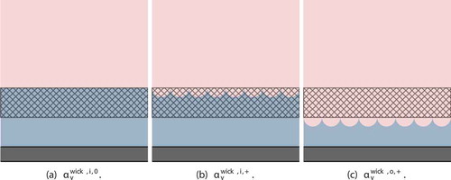
The contact angle of the liquid-vapor interface is critical for computing the capillary pressure $\mathrm{\Delta }{p}_{\mathrm{c}\mathrm{a}\mathrm{p}}$ and the interfacial area density $a_{\mathrm{i}\mathrm{n}\mathrm{t}}$. The contact angle is determined from the void fraction ${\alpha }_v$. First, a number of bounds in ${\alpha }_v$ are defined, which are described as follows:

1. ${\alpha }_v^{\mathrm{w}\mathrm{i}\mathrm{c}\mathrm{k},\mathrm{i},0}$: Interface is flat at the inner wick surface.

2. ${\alpha }_v^{\mathrm{w}\mathrm{i}\mathrm{c}\mathrm{k},\mathrm{i},+}$: Interface is at the inner wick surface, with hemispherical vapor pore volumes receding into wick.

3. ${\alpha }_v^{\mathrm{w}\mathrm{i}\mathrm{c}\mathrm{k},\mathrm{o},+}$: Interface is at the outer wick surface, with hemispherical vapor pore volumes receding into wick.

These bounds are illustrated in Fig. 3 and are computed as follows:

(33a) ${\alpha }_v^{\mathrm{w}\mathrm{i}\mathrm{c}\mathrm{k},\mathrm{i},0}=\frac{A_{\mathrm{c}\mathrm{o}\mathrm{r}\mathrm{e}}}{A},$(33a)

(33b) ${\alpha }_v^{\mathrm{w}\mathrm{i}\mathrm{c}\mathrm{k},\mathrm{i},+}={\alpha }_v^{\mathrm{w}\mathrm{i}\mathrm{c}\mathrm{k},\mathrm{i},0}+N{{ }^{\mathrm{\prime }\mathrm{\prime }\mathrm{\prime }}}_{\mathrm{p}\mathrm{o}\mathrm{r}\mathrm{e}}(D_{\mathrm{w}\mathrm{i}\mathrm{c}\mathrm{k},\mathrm{i}})V_{\mathrm{p}\mathrm{o}\mathrm{r}\mathrm{e},\mathrm{h}\mathrm{e}\mathrm{m}\mathrm{i}},$(33b)

Fig. 3. Void fraction bounds illustration. Vapor is shown in pink, liquid in blue, and cladding in gray

and

(33c) ${\alpha }_v^{\mathrm{w}\mathrm{i}\mathrm{c}\mathrm{k},\mathrm{o},+}=\frac{A_{\mathrm{c}\mathrm{o}\mathrm{r}\mathrm{e}}+\phi A_{\mathrm{w}\mathrm{i}\mathrm{c}\mathrm{k}}}{A}+N{{ }^{\mathrm{\prime }\mathrm{\prime }\mathrm{\prime }}}_{\mathrm{p}\mathrm{o}\mathrm{r}\mathrm{e}}(D_{\mathrm{w}\mathrm{i}\mathrm{c}\mathrm{k},\mathrm{o}})V_{\mathrm{p}\mathrm{o}\mathrm{r}\mathrm{e},\mathrm{h}\mathrm{e}\mathrm{m}\mathrm{i}},$(33c)

where $V_{\mathrm{p}\mathrm{o}\mathrm{r}\mathrm{e},\mathrm{h}\mathrm{e}\mathrm{m}\mathrm{i}}=\frac{2}{3}\pi R_{\mathrm{p}\mathrm{o}\mathrm{r}\mathrm{e}}^3$ represents the hemispherical volume of a single pore. The pore site density function $N{{ }^{\mathrm{\prime }\mathrm{\prime }\mathrm{\prime }}}_{\mathrm{p}\mathrm{o}\mathrm{r}\mathrm{e}}(D)$ computes, for a diameter $D$ within the wick, the number of pore sites per unit flow volume of the entire heat pipe cross section. It is defined by assuming the porosity $\phi$ to be valid as a surface porosity, not just a volume porosity:

(34) $N{{ }^{\mathrm{\prime }\mathrm{\prime }\mathrm{\prime }}}_{\mathrm{p}\mathrm{o}\mathrm{r}\mathrm{e}}(D)=\frac{\phi \pi D}{A_{\mathrm{p}\mathrm{o}\mathrm{r}\mathrm{e}}A},$(34)

where $A_{\mathrm{p}\mathrm{o}\mathrm{r}\mathrm{e}}=\pi R_{\mathrm{p}\mathrm{o}\mathrm{r}\mathrm{e}}^2$ denotes the individual pore cross-sectional area.

The contact angle ${\theta }_{\mathrm{c}\mathrm{a}\mathrm{p}}$ of the liquid-vapor interface is defined such that

(35) $cos{\theta }_{\mathrm{c}\mathrm{a}\mathrm{p}}=\frac{R_{\mathrm{p}\mathrm{o}\mathrm{r}\mathrm{e}}}{R_{\mathrm{c}\mathrm{a}\mathrm{p}}},$(35)

where $R_{\mathrm{c}\mathrm{a}\mathrm{p}}$ is the capillary radius, or radius of curvature, of the interface. Figure 4 gives an illustration of the contact angle.

Fig. 4. Contact angle definition. Vapor is shown in pink, liquid in blue, and wick in gray

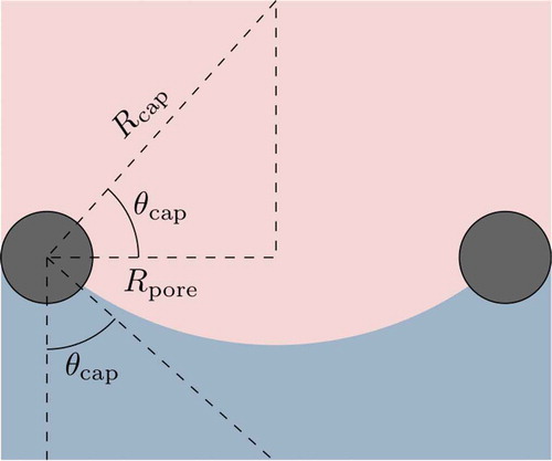
Let $\xi$ denote the sine of the contact angle:

(36) $\xi \equiv sin{\theta }_{\mathrm{c}\mathrm{a}\mathrm{p}}.$(36)

Combining this with Eq. (35)(35) $cos{\theta }_{\mathrm{c}\mathrm{a}\mathrm{p}}=\frac{R_{\mathrm{p}\mathrm{o}\mathrm{r}\mathrm{e}}}{R_{\mathrm{c}\mathrm{a}\mathrm{p}}},$(35) gives the capillary radius as a function of $\xi$:

(37) $R_{\mathrm{c}\mathrm{a}\mathrm{p}}(\xi )=\frac{R_{\mathrm{p}\mathrm{o}\mathrm{r}\mathrm{e}}}{cos{\theta }_{\mathrm{c}\mathrm{a}\mathrm{p}}}=\frac{R_{\mathrm{p}\mathrm{o}\mathrm{r}\mathrm{e}}}{\sqrt{1-{\xi }^2}}.$(37)

For the cases ${\alpha }_v\le {\alpha }_v^{\mathrm{w}\mathrm{i}\mathrm{c}\mathrm{k},\mathrm{i},0}$ and ${\alpha }_v>{\alpha }_v^{\mathrm{w}\mathrm{i}\mathrm{c}\mathrm{k},\mathrm{o},+}$, the interface is assumed to be flat. For the case ${\alpha }_v^{\mathrm{w}\mathrm{i}\mathrm{c}\mathrm{k},\mathrm{i},+}<{\alpha }_v\le {\alpha }_v^{\mathrm{w}\mathrm{i}\mathrm{c}\mathrm{k},\mathrm{o},+}$, the interface is fully curved toward the heat pipe wall. Finally, for the case ${\alpha }_v^{\mathrm{w}\mathrm{i}\mathrm{c}\mathrm{k},\mathrm{i},0}<{\alpha }_v\le {\alpha }_v^{\mathrm{w}\mathrm{i}\mathrm{c}\mathrm{k},\mathrm{i},+}$, the interface has a radius of curvature between $R_{\mathrm{p}\mathrm{o}\mathrm{r}\mathrm{e}}$ (full hemisphere) and infinity (flat). Applying these concepts,

(38a) $\xi ({\alpha }_v)=\left\{\begin{array}{cc}1& {\alpha }_v\le {\alpha }_v^{\mathrm{w}\mathrm{i}\mathrm{c}\mathrm{k},\mathrm{i},0}\\ \frac{1}{C_2}+\frac{C_2}{C_1+1}-1& {\alpha }_v^{\mathrm{w}\mathrm{i}\mathrm{c}\mathrm{k},\mathrm{i},0}<{\alpha }_v<{\alpha }_v^{\mathrm{w}\mathrm{i}\mathrm{c}\mathrm{k},\mathrm{i},+}\\ 0& {\alpha }_v^{\mathrm{w}\mathrm{i}\mathrm{c}\mathrm{k},\mathrm{i},+}\le {\alpha }_v<{\alpha }_v^{\mathrm{w}\mathrm{i}\mathrm{c}\mathrm{k},\mathrm{o},+}\\ 1& {\alpha }_v\ge {\alpha }_v^{\mathrm{w}\mathrm{i}\mathrm{c}\mathrm{k},\mathrm{o},+}\end{array}\right.,$(38a)

(38b) $C_1({\alpha }_v)={\left(\frac{3\left({\alpha }_v-{\alpha }_v^{\mathrm{w}\mathrm{i}\mathrm{c}\mathrm{k},\mathrm{i},0}\right)}{\pi R_{\mathrm{p}\mathrm{o}\mathrm{r}\mathrm{e}}^3{N{ }^{\mathrm{\prime }\mathrm{\prime }\mathrm{\prime }}}_{\mathrm{p}\mathrm{o}\mathrm{r}\mathrm{e}}(D_{\mathrm{w}\mathrm{i}\mathrm{c}\mathrm{k},\mathrm{i}})}\right)}^2,$(38b)

and

(38c) $C_2({\alpha }_v)=\sqrt[3]{{(C_1+1)}^2+\sqrt{C_1\left(1+C_1\left(3+C_1\left(3+C_1\right)\right)\right)}}.$(38c)

The expression for the case ${\alpha }_v^{\mathrm{w}\mathrm{i}\mathrm{c}\mathrm{k},\mathrm{i},0}<{\alpha }_v<{\alpha }_v^{\mathrm{w}\mathrm{i}\mathrm{c}\mathrm{k},\mathrm{i},+}$ is derived using the geometric relation of the void volume of each pore as a function of $\xi$:

(39) $V_{\mathrm{p}\mathrm{o}\mathrm{r}\mathrm{e}}(\xi )=\frac{\pi R_{\mathrm{p}\mathrm{o}\mathrm{r}\mathrm{e}}^3}{3}\left(2+\xi \right)\sqrt{\frac{1-\xi }{{\left(1+\xi \right)}^3}}.$(39)

This expression, combined with the following void fraction relation, is inverted to give the expression in Eq. (38)(36) $\xi \equiv sin{\theta }_{\mathrm{c}\mathrm{a}\mathrm{p}}.$(36) :

(40) ${\alpha }_v(\xi )={\alpha }_v^{\mathrm{w}\mathrm{i}\mathrm{c}\mathrm{k},\mathrm{i},0}+N{{ }^{\mathrm{\prime }\mathrm{\prime }\mathrm{\prime }}}_{\mathrm{p}\mathrm{o}\mathrm{r}\mathrm{e}}(D_{\mathrm{w}\mathrm{i}\mathrm{c}\mathrm{k},\mathrm{i}})V_{\mathrm{p}\mathrm{o}\mathrm{r}\mathrm{e}}(\xi ).$(40)

II.A.2. Capillary Pressure

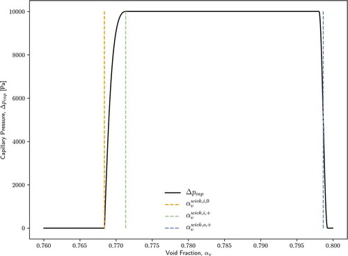
The capillary pressure difference between the phases is a function of the capillary radius:

(41) $\mathrm{\Delta }{p}_{\mathrm{c}\mathrm{a}\mathrm{p}}({\alpha }_v)=\left\{\begin{array}{cc}0& \xi =1\\ \frac{{\displaystyle 2\sigma }}{{\displaystyle R_{\mathrm{c}\mathrm{a}\mathrm{p}}(\xi )}}& \xi \ne 1\end{array}\right..$(41)

Figure 5 shows an example of the capillary pressure dependence on void fraction. Note that a smoothing process is performed at the discontinuity at ${\alpha }_v={\alpha }_v^{\mathrm{w}\mathrm{i}\mathrm{c}\mathrm{k},\mathrm{o},+}$.

Fig. 5. Capillary pressure versus void fraction

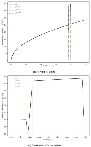
II.A.3. Interfacial Area Density

The interfacial area density $a_{\mathrm{i}\mathrm{n}\mathrm{t}}$ represents the surface area of the liquid-vapor interface per unit flow volume. The bounding void fraction values discussed in Sec. II.A.1 determine the regime of the interfacial area density:

1. For ${\alpha }_v\le {\alpha }_v^{\mathrm{w}\mathrm{i}\mathrm{c}\mathrm{k},\mathrm{i},0}$, the liquid-vapor interface is a cylindrical surface within the core region around the cross-section ${\alpha }_{v}A$.

2. For ${\alpha }_v^{\mathrm{w}\mathrm{i}\mathrm{c}\mathrm{k},\mathrm{i},0}<{\alpha }_v\le {\alpha }_v^{\mathrm{w}\mathrm{i}\mathrm{c}\mathrm{k},\mathrm{i},+}$, the liquid-vapor interface is composed of interface areas in all of the pores, with an individual surface area $S_{\mathrm{p}\mathrm{o}\mathrm{r}\mathrm{e}}(\xi )$:

(42) $S_{\mathrm{p}\mathrm{o}\mathrm{r}\mathrm{e}}(\xi )=\frac{2\pi R_{\mathrm{p}\mathrm{o}\mathrm{r}\mathrm{e}}^2}{1+\xi }.$(42)

3. For ${\alpha }_v^{\mathrm{w}\mathrm{i}\mathrm{c}\mathrm{k},\mathrm{i},+}<{\alpha }_v\le {\alpha }_v^{\mathrm{w}\mathrm{i}\mathrm{c}\mathrm{k},\mathrm{o},+}$, the liquid-vapor interface is again composed of interface areas in all of the pores, but now $\xi =1$ and is not a function of ${\alpha }_v$. To find the diameter of the interfaces $D_{\mathrm{i}\mathrm{n}\mathrm{t}}$ between the wick inner and outer diameter, the following expression for void fraction in this region is inverted:

(43) ${\alpha }_v={\alpha }_v^{\mathrm{w}\mathrm{i}\mathrm{c}\mathrm{k},\mathrm{i},0}+\frac{\phi \pi (D_{\mathrm{i}\mathrm{n}\mathrm{t}}^2-D_{\mathrm{w}\mathrm{i}\mathrm{c}\mathrm{k},\mathrm{i}}^2)}{4A}+N{{ }^{\mathrm{\prime }\mathrm{\prime }\mathrm{\prime }}}_{\mathrm{p}\mathrm{o}\mathrm{r}\mathrm{e}}(D_{\mathrm{i}\mathrm{n}\mathrm{t}})V_{\mathrm{p}\mathrm{o}\mathrm{r}\mathrm{e},\mathrm{h}\mathrm{e}\mathrm{m}\mathrm{i}},$(43)

where the second term accounts for the flow area between this diameter and the wick inner diameter.

4. For ${\alpha }_v>{\alpha }_v^{\mathrm{w}\mathrm{i}\mathrm{c}\mathrm{k},\mathrm{o},+}$, the liquid-vapor interface is a cylindrical surface within the liquid annulus. The diameter of this surface is found by using the fact that the liquid area is $(1-{\alpha }_v)A$ and that the outer diameter of the annulus area is $D_{\mathrm{c}\mathrm{l}\mathrm{a}\mathrm{d},\mathrm{i}}$.

Putting this all together,

(44a) $a_{\mathrm{i}\mathrm{n}\mathrm{t}}({\alpha }_v)=\left\{\begin{array}{cc}\frac{2\pi }{A}\sqrt{\frac{{\alpha }_{v}A}{\pi }}& {\alpha }_v\le {\alpha }_v^{\mathrm{w}\mathrm{i}\mathrm{c}\mathrm{k},\mathrm{i},0}\\ \frac{2\pi R_{\mathrm{p}\mathrm{o}\mathrm{r}\mathrm{e}}^2{N{ }^{\mathrm{\prime }\mathrm{\prime }\mathrm{\prime }}}_{\mathrm{p}\mathrm{o}\mathrm{r}\mathrm{e}}(D_{\mathrm{w}\mathrm{i}\mathrm{c}\mathrm{k},\mathrm{i}})}{1+\xi }& {\alpha }_v^{\mathrm{w}\mathrm{i}\mathrm{c}\mathrm{k},\mathrm{i},0}<{\alpha }_v\le {\alpha }_v^{\mathrm{w}\mathrm{i}\mathrm{c}\mathrm{k},\mathrm{i},+}\\ 2\pi R_{\mathrm{p}\mathrm{o}\mathrm{r}\mathrm{e}}^2{N{ }^{\mathrm{\prime }\mathrm{\prime }\mathrm{\prime }}}_{\mathrm{p}\mathrm{o}\mathrm{r}\mathrm{e}}(D_{\mathrm{i}\mathrm{n}\mathrm{t}})& {\alpha }_v^{\mathrm{w}\mathrm{i}\mathrm{c}\mathrm{k},\mathrm{i},+}<{\alpha }_v\le {\alpha }_v^{\mathrm{w}\mathrm{i}\mathrm{c}\mathrm{k},0,+}\\ \frac{\pi }{A}\sqrt{D_{\mathrm{c}\mathrm{l}\mathrm{a}\mathrm{d},\mathrm{i}}^2-\frac{4(1-{\alpha }_v)A}{\pi }}& {\alpha }_v>{\alpha }_v^{\mathrm{w}\mathrm{i}\mathrm{c}\mathrm{k},\mathrm{o},+}\end{array}\right.$(44a)

and

$D_{\mathrm{i}\mathrm{n}\mathrm{t}}=\frac{-b+\sqrt{b^2-4ac}}{2a},\left\{\begin{array}{c}a=\frac{\phi \pi }{4}\\ b=\frac{\phi \pi V_{\mathrm{p}\mathrm{o}\mathrm{r}\mathrm{e},\mathrm{h}\mathrm{e}\mathrm{m}\mathrm{i}}}{A_{\mathrm{p}\mathrm{o}\mathrm{r}\mathrm{e}}}\\ c=({\alpha }_v^{\mathrm{w}\mathrm{i}\mathrm{c}\mathrm{k},\mathrm{i},0}-{\alpha }_v)A-\frac{\phi \pi D_{\mathrm{w}\mathrm{i}\mathrm{c}\mathrm{k},\mathrm{i}}^2}{4}\end{array}\right..(44\mathrm{b})$

Figure 6 shows how the interfacial area density varies with void fraction. Similar to the capillary pressure, a smoothing process is performed at the discontinuities at ${\alpha }_v={\alpha }_v^{\mathrm{w}\mathrm{i}\mathrm{c}\mathrm{k},\mathrm{i},0}$ and ${\alpha }_v={\alpha }_v^{\mathrm{w}\mathrm{i}\mathrm{c}\mathrm{k},\mathrm{o},+}$.

Fig. 6. Interfacial area density versus void fraction

II.A.4. Thermodynamic Properties

Sockeye can be used with a generic equation of state. Currently, Sockeye provides equations of state for sodium and potassium as the working fluids.

The fluid properties of liquid sodium are obtained by integrating the compressibility equation by Gupta²⁸ from the saturated liquid state to the given state point. Vapor and saturation properties for sodium are given by Golden and Tokar.²⁹

The fluid properties of potassium vapor are calculated with the same model that Golden and Tokar introduced for sodium, whereas the coefficients for potassium are given in Ref. 30. For the liquid phase of potassium, no trusted compressibility equation was found in the literature; therefore, the calculation of the compressibility is carried out using a corresponding-states law for the compressibility of alkali metals given by Pasternak.³¹

II.A.5. Operational Limits

Heat pipes are subject to a number of phenomena that limit their heat transport capability. The most commonly cited operational limits are the following^1,2:

1. Capillary: Capillary pressure is insufficient to draw liquid into the evaporator region, leading to dryout.

2. Viscous: Viscous pressure losses may be dominant for the vapor flow, and the vapor pressure may reduce to zero.

3. Sonic: Comparable to a converging-diverging nozzle, a choked condition can develop at the evaporator exit, limiting the vapor speed at this point to the local speed of sound.

4. Entrainment: Liquid from the inner wick surface is sheared off by the vapor flow and taken to the condenser end, possibly leading to dryout.

5. Boiling: Excessive radial heat flux causes liquid in the wick to boil and possibly leads to dryout.

The flow model in Sockeye does not explicitly compute these limitations; instead, these limits are intended to be reproduced by the physics inherent in the flow model. When the capillary limit is encountered, the evaporator should dry out due to insufficient liquid return. When the sonic limit is encountered, choked flow at the evaporator exit should be observed. When the viscous limit is encountered, a near-zero pressure value should be observed at the condenser end of the vapor channel, inhibiting the movement of the vapor phase. Entrainment and boiling limits will require additional models to capture their effects, but it has been noted that for liquid metal heat pipes, both of these limits are rarely encountered.² Demonstration of the capillary, viscous, and sonic limits is a planned future task; see Sec. IV.

II.B. Heat Conduction

Sockeye also models 2-D heat conduction in axisymmetric coordinates, such as that in the heat pipe cladding, or additional bodies in contact with the heat pipe. Given the spatial domain $\mathrm{\Omega }=(r_1,r_2)\times (x_1,x_2)$ and its boundary $\mathrm{\partial }\mathrm{\Omega }$, the strong form of the heat conduction problem is the following:

(45) $\rho c_p\frac{\mathrm{\partial }T}{\mathrm{\partial }t}-\mathrm{\nabla }\cdot (k\mathrm{\nabla }T)=0(r,x)\in \mathrm{\Omega },$(45)

(46) $T(r,x,t=0)=T_0(r,x)(r,x)\in \mathrm{\Omega },$(46)

and

(47) $q(r,x,t)\equiv -k\mathrm{\nabla }T=q_b(r,x,t)(r,x)\in \mathrm{\partial }\mathrm{\Omega },$(47)

where $T_0$ is an initial temperature function, and $q_b$ is a boundary flux function. Table I summarizes the different boundary condition options, which can be applied to the boundaries $r=r_1$ and $r=r_2$ independently, as well as in specific axial regions. For the radiation boundary condition, $\epsilon$ represents the surface emissivity, $\sigma$ is the Stefan-Boltzmann constant, and $F$ is the view factor. The boundaries $x=x_1$ and $x=x_2$ are assumed to be insulated.

TABLE I Heat Conduction Boundary Conditions

Boundary Condition	Flux Function
Insulated	$q_b=0$
Direct heat flux	$q_b=q_b(r,x,t)$
Flow coupling	$q_b=\mathcal{H}(T_{\mathrm{\ell }}-T)$
Convection	$q_b=\mathcal{H}(T_{\mathrm{\infty }}-T)$
Radiation	$q_b=\epsilon \sigma F(T_{\mathrm{\infty }}^4-T^4)$
Combination	$q_b=\sum _i{q}_{b,i}$

III. DISCRETIZATION

III.A. Spatial Discretization

The flow equations given by Eqs. (5)(5) $\frac{\mathrm{\partial }{\alpha }_{\mathrm{\ell }}A}{\mathrm{\partial }t}+u_{\mathrm{i}\mathrm{n}\mathrm{t}}\frac{\mathrm{\partial }{\alpha }_{\mathrm{\ell }}}{\mathrm{\partial }x}A=\mathrm{\Theta }\left(p_{\mathrm{\ell }}+\mathrm{\Delta }{p}_{\mathrm{c}\mathrm{a}\mathrm{p}}-p_v\right)A-\frac{{\mathrm{\Gamma }}_{\mathrm{i}\mathrm{n}\mathrm{t}}{a}_{\mathrm{i}\mathrm{n}\mathrm{t}}A}{{\rho }_{\mathrm{i}\mathrm{n}\mathrm{t}}},$(5) through (11(11) $\begin{array}{rl}& \frac{\mathrm{\partial }{\alpha }_v{\rho }_v{E}_{v}A}{\mathrm{\partial }t}+\frac{\mathrm{\partial }{\alpha }_v{u}_v\left({\rho }_v{E}_v+p_v\right)A}{\mathrm{\partial }x}=p_{\mathrm{i}\mathrm{n}\mathrm{t}}{u}_{\mathrm{i}\mathrm{n}\mathrm{t}}\frac{\mathrm{\partial }{\alpha }_v}{\mathrm{\partial }x}A\\ & +{\bar{p}}_{\mathrm{i}\mathrm{n}\mathrm{t}}\mathrm{\Theta }\left(p_{\mathrm{\ell }}+\mathrm{\Delta }{p}_{\mathrm{c}\mathrm{a}\mathrm{p}}-p_v\right)A+{\alpha }_v{\rho }_v{g}_x{u}_{v}A\\ & +q_v^{\mathrm{w}\mathrm{a}\mathrm{l}\mathrm{l}}{P}_{\mathrm{w}\mathrm{a}\mathrm{l}\mathrm{l}}+q_v^{\mathrm{i}\mathrm{n}\mathrm{t}}{a}_{\mathrm{i}\mathrm{n}\mathrm{t}}A+{\mathrm{\Gamma }}_{\mathrm{i}\mathrm{n}\mathrm{t}}{E}_v^{\mathrm{i}\mathrm{n}\mathrm{t}}{a}_{\mathrm{i}\mathrm{n}\mathrm{t}}A.\end{array}$(11) ) are discretized using a finite volume scheme with optional slope reconstruction and total variation diminishing limitation.^32,33 When slope reconstruction is omitted, the scheme reduces to a Godunov scheme. Spatial discretization is an extensive subject and is not the focus of this work; therefore, only an overview is given here, and details are left to other references. First, the flow equations are expressed in the following form:

(48a) $\frac{\mathrm{\partial }\mathbf{U}}{\mathrm{\partial }t}+\frac{\mathrm{\partial }\mathbf{F}(\mathbf{U})}{\mathrm{\partial }x}+\mathrm{d}\mathrm{i}\mathrm{a}\mathrm{g}(\alpha (\mathbf{U}))\frac{\mathrm{\partial }\mathbf{H}(\mathbf{U})}{\mathrm{\partial }x}=\mathbf{S}(\mathbf{U}),$(48a)

(48b) $\mathbf{U}\equiv \left[\begin{array}{c}{\alpha }_{\mathrm{\ell }}A\\ {\alpha }_{\mathrm{\ell }}{\rho }_{\mathrm{\ell }}A\\ {\alpha }_{\mathrm{\ell }}{\rho }_{\mathrm{\ell }}{u}_{\mathrm{\ell }}A\\ {\alpha }_{\mathrm{\ell }}{\rho }_{\mathrm{\ell }}{E}_{\mathrm{\ell }}A\\ {\alpha }_v{\rho }_{v}A\\ {\alpha }_v{\rho }_v{u}_{v}A\\ {\alpha }_v{\rho }_v{E}_{v}A\end{array}\right],\mathbf{F}(\mathbf{U})\equiv \left[\begin{array}{c}{\alpha }_{\mathrm{\ell }}{u}_{\mathrm{i}\mathrm{n}\mathrm{t}}A\\ {\alpha }_{\mathrm{\ell }}{\rho }_{\mathrm{\ell }}{u}_{\mathrm{\ell }}A\\ {\alpha }_{\mathrm{\ell }}({\rho }_{\mathrm{\ell }}{u}_{\mathrm{\ell }}^2+p_{\mathrm{\ell }})A-{\alpha }_{\mathrm{\ell }}{p}_{\mathrm{i}\mathrm{n}\mathrm{t}}A\\ {\alpha }_{\mathrm{\ell }}{u}_{\mathrm{\ell }}({\rho }_{\mathrm{\ell }}{E}_{\mathrm{\ell }}+p_{\mathrm{\ell }})A-{\alpha }_{\mathrm{\ell }}{p}_{\mathrm{i}\mathrm{n}\mathrm{t}}{u}_{\mathrm{i}\mathrm{n}\mathrm{t}}A-{\alpha }_{\mathrm{\ell }}{k}_{\mathrm{\ell }}\frac{\mathrm{\partial }{T}_{\mathrm{\ell }}}{\mathrm{\partial }x}A\\ {\alpha }_v{\rho }_v{u}_{v}A\\ {\alpha }_v({\rho }_v{u}_v^2+p_v)A-{\alpha }_v{p}_{\mathrm{i}\mathrm{n}\mathrm{t}}A\\ {\alpha }_v{u}_v({\rho }_v{E}_v+p_v)A-{\alpha }_v{p}_{\mathrm{i}\mathrm{n}\mathrm{t}}{u}_{\mathrm{i}\mathrm{n}\mathrm{t}}A\end{array}\right],$(48b)

and

(48c) $\alpha (\mathbf{U})\equiv \left[\begin{array}{c}{\alpha }_{\mathrm{\ell }}\\ {\alpha }_{\mathrm{\ell }}\\ {\alpha }_{\mathrm{\ell }}\\ {\alpha }_{\mathrm{\ell }}\\ {\alpha }_v\\ {\alpha }_v\\ {\alpha }_v\end{array}\right],\mathbf{H}(\mathbf{U})\equiv \left[\begin{array}{c}-u_{\mathrm{i}\mathrm{n}\mathrm{t}}A\\ 0\\ p_{\mathrm{i}\mathrm{n}\mathrm{t}}A\\ p_{\mathrm{i}\mathrm{n}\mathrm{t}}{u}_{\mathrm{i}\mathrm{n}\mathrm{t}}A\\ 0\\ p_{\mathrm{i}\mathrm{n}\mathrm{t}}A\\ p_{\mathrm{i}\mathrm{n}\mathrm{t}}{u}_{\mathrm{i}\mathrm{n}\mathrm{t}}A\end{array}\right],$(48c)

and for brevity, $\mathbf{S}(\mathbf{U})$ is left to be inferred from the remaining terms in Eqs. (5)(5) $\frac{\mathrm{\partial }{\alpha }_{\mathrm{\ell }}A}{\mathrm{\partial }t}+u_{\mathrm{i}\mathrm{n}\mathrm{t}}\frac{\mathrm{\partial }{\alpha }_{\mathrm{\ell }}}{\mathrm{\partial }x}A=\mathrm{\Theta }\left(p_{\mathrm{\ell }}+\mathrm{\Delta }{p}_{\mathrm{c}\mathrm{a}\mathrm{p}}-p_v\right)A-\frac{{\mathrm{\Gamma }}_{\mathrm{i}\mathrm{n}\mathrm{t}}{a}_{\mathrm{i}\mathrm{n}\mathrm{t}}A}{{\rho }_{\mathrm{i}\mathrm{n}\mathrm{t}}},$(5) through (11)(11) $\begin{array}{rl}& \frac{\mathrm{\partial }{\alpha }_v{\rho }_v{E}_{v}A}{\mathrm{\partial }t}+\frac{\mathrm{\partial }{\alpha }_v{u}_v\left({\rho }_v{E}_v+p_v\right)A}{\mathrm{\partial }x}=p_{\mathrm{i}\mathrm{n}\mathrm{t}}{u}_{\mathrm{i}\mathrm{n}\mathrm{t}}\frac{\mathrm{\partial }{\alpha }_v}{\mathrm{\partial }x}A\\ & +{\bar{p}}_{\mathrm{i}\mathrm{n}\mathrm{t}}\mathrm{\Theta }\left(p_{\mathrm{\ell }}+\mathrm{\Delta }{p}_{\mathrm{c}\mathrm{a}\mathrm{p}}-p_v\right)A+{\alpha }_v{\rho }_v{g}_x{u}_{v}A\\ & +q_v^{\mathrm{w}\mathrm{a}\mathrm{l}\mathrm{l}}{P}_{\mathrm{w}\mathrm{a}\mathrm{l}\mathrm{l}}+q_v^{\mathrm{i}\mathrm{n}\mathrm{t}}{a}_{\mathrm{i}\mathrm{n}\mathrm{t}}A+{\mathrm{\Gamma }}_{\mathrm{i}\mathrm{n}\mathrm{t}}{E}_v^{\mathrm{i}\mathrm{n}\mathrm{t}}{a}_{\mathrm{i}\mathrm{n}\mathrm{t}}A.\end{array}$(11) .

Integrating over each cell volume $\mathrm{\Delta }{x}_i$, approximating the third term on the left side of Eq. (48a)(48a) $\frac{\mathrm{\partial }\mathbf{U}}{\mathrm{\partial }t}+\frac{\mathrm{\partial }\mathbf{F}(\mathbf{U})}{\mathrm{\partial }x}+\mathrm{d}\mathrm{i}\mathrm{a}\mathrm{g}(\alpha (\mathbf{U}))\frac{\mathrm{\partial }\mathbf{H}(\mathbf{U})}{\mathrm{\partial }x}=\mathbf{S}(\mathbf{U}),$(48a) by assuming $\alpha ={\alpha }_i$ over $\mathrm{\Delta }{x}_i$, using the divergence theorem, and then approximating the inter-cell fluxes gives a finite volume discretization:

(49a) $|\mathrm{\Delta }{x}_i|\frac{\mathrm{d}{\mathbf{U}}_i}{\mathrm{d}t}+{\mathbf{F}}_{i+1/2,i}-{\mathbf{F}}_{i-1/2,i}+\mathrm{d}\mathrm{i}\mathrm{a}\mathrm{g}({\alpha }_i)\left({\mathbf{H}}_{i+1/2,i}-{\mathbf{H}}_{i-1/2,i}\right)\approx \underset{\mathrm{\Delta }{x}_i}{\int }\mathbf{S}\mathrm{d}x,$(49a)

${\mathbf{U}}_i(t)\equiv \frac{1}{|\mathrm{\Delta }{x}_i|}\underset{\mathrm{\Delta }{x}_i}{\int }\mathbf{U}(x,t)\mathrm{d}x,{\alpha }_i(t)\equiv \frac{1}{|\mathrm{\Delta }{x}_i|}\underset{\mathrm{\Delta }{x}_i}{\int }\alpha (x,t)\mathrm{d}x,(49b)$

and

${\mathbf{F}}_{i+1/2,i}(t)\approx \mathbf{F}(\mathbf{U}(x_{i+1/2},t)),{\mathbf{H}}_{i+1/2,i}(t)\approx \mathbf{H}(\mathbf{U}(x_{i+1/2},t)).(49c)$

The computation of the numerical fluxes ${\mathbf{F}}_{i+1/2,i}$ and ${\mathbf{H}}_{i+1/2,i}$ is performed using an approximate Riemann solver, the details of which can be found in Ref. 34 and are not duplicated here.

The heat conduction equation given by Eq. (45)(45) $\rho c_p\frac{\mathrm{\partial }T}{\mathrm{\partial }t}-\mathrm{\nabla }\cdot (k\mathrm{\nabla }T)=0(r,x)\in \mathrm{\Omega },$(45) is discretized using the continuous finite element method; after integration by parts, the following weak form is obtained:

(50) ${\left(\rho c_p\frac{\mathrm{\partial }T}{\mathrm{\partial }t},{\varphi }_i\right)}_{\mathrm{\Omega }}+{\left(k\mathrm{\nabla }T,\mathrm{\nabla }{\varphi }_i\right)}_{\mathrm{\Omega }}-{⟨k\mathrm{\nabla }T,{\varphi }_i\mathbf{n}⟩}_{\mathrm{\partial }\mathrm{\Omega }}=0,$(50)

where $(\cdot ,\cdot {)}_{\mathrm{\Omega }}$ denotes a volume integral over $\mathrm{\Omega }$, and ${⟨\cdot ,\cdot ⟩}_{\mathrm{\partial }\mathrm{\Omega }}$ denotes a surface integral over the boundary of $\mathrm{\Omega }$.

III.B. Temporal Discretization

Sockeye supports both explicit and implicit temporal discretizations. Heat pipe transients of interest typically feature time domains on the scale of seconds to hours, for which the use of explicit temporal discretizations is impractical due to the Courant-Friedrichs-Lewy time-step size restriction. Therefore, implicit methods are usually more appropriate. The recommended implicit temporal discretization is the second-order Backward Difference Formula (BDF2), which is L-stable and thus suitable for integration of stiff equations.³⁵ For an ordinary differential equation,

(51) $\frac{\mathrm{\partial }u}{\mathrm{\partial }t}=f(u,t),$(51)

the BDF2 update step can be expressed as

(52) $u^{n+1}=\frac{4}{3}{u}^n-\frac{1}{3}{u}^{n-1}+\frac{2}{3}\mathrm{\Delta }tf(u^{n+1},t^{n+1}).$(52)

IV. VERIFICATION AND VALIDATION

Development of a verification and validation plan for Sockeye is currently underway. Verification will include a number of tasks such as verification of conservation of mass and energy and reproduction of analytic velocity and pressure profiles and temperature values.

The collection of experimental data for high-temperature heat pipes is challenging. Instrumentation must be able to withstand these high temperatures, and installation of instrumentation on the inside of a heat pipe potentially affects the flow field. Most experimental data for high-temperature heat pipes is limited to externally mounted thermocouples; however, some experimentalists have measured internal data, such as vapor temperature.^36,37 The following past experiments have been identified as potential validation cases:

1. SAFE-30 heat pipe module test⁷: In this experiment, a sodium/stainless steel heat pipe was attached to four cartridge heaters in a vacuum chamber. Thermocouples were mounted on three locations on the “fuel” tubes containing the cartridge heaters and five axial locations on the surface of the heat pipe cladding. A 5-h power ramp-up (to 2600 W electrical power) and cooldown was performed from the frozen state. The thermocouple data and measured powers have been provided to the Sockeye team. A preliminary comparison to these data is provided in Sec. V.B.

2. High-temperature heat pipes with multiple heat sources^36,37: In these experiments, a sodium/stainless steel heat pipe designed to operate in a vapor temperature range of 500°C to 800°C was fitted with four heaters (in different axial sections) and subjected to different combinations of powers to each. Additional dimensions to the experiments included the ambient condition (air versus vacuum), the working fluid fill level (two cases were tested), and the inclination of the heat pipe with respect to gravity (a few angles near the horizontal were tested). Data were collected from 12 wall thermocouples, 6 vapor space thermocouples, and calorimeters in the evaporator, transport, and condenser sections. Regimes studied include startup, continuum transient, and steady state.

In addition to existing heat pipe data, two Nuclear Energy University Program (NEUP) experimental studies are scheduled to produce data that will support Sockeye validation:

1. NEUP Project 20-19735—Experiments for Modeling and Validation of Liquid-Metal Heat Pipe Simulation Tools for Micro-Reactors³⁸: Normal operation, as well as the transient behavior of frozen startup, shutdown, and restart will be studied. The temperature distribution in the core, wick, annular gap, and external wall surface will be measured by a fiber-optic distributed temperature sensor and thermocouples. Pressure will be measured using pressure-transfer-liquid techniques. Phase distribution will be measured using X-ray systems.

2. NEUP Project 19-17416—Experiments and Computations to Address the Safety Case of Heat Pipe Failures in Special Purpose Reactors³⁹: Startup, shutdown, and normal operation will be studied at different inclinations. Thermocouples and optic fibers will be installed in all axial regions on the outside of the heat pipe. High-resolution X-ray imaging will be used to measure void fraction.

V. NUMERICAL DEMONSTRATIONS

This section gives numerical demonstrations of some of Sockeye’s capabilities to show that heat pipe operational phenomena are observed. Section V.A gives an example of comparing a single-ended configuration to a double-ended configuration and compares to some analytic solutions. Section V.B shows some modeling of the SAFE-30 heat pipe module test and compares to experimental data. Section V.C demonstrates spatial convergence using a manufactured solution. All runs were performed using Sockeye, version pub/nt-2020-rev1.

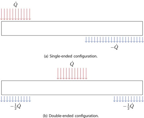
V.A. Test A: Double-Ended Heat Pipe

In this test problem, a comparison is made between single-ended and double-ended configurations for a heat pipe. Table II summarizes the heat pipe parameters and conditions used for this test problem. The input thermal power is imposed directly and uniformly over the evaporator and equally removed from the condenser region(s). For the single-ended configuration, the evaporator is along the first 0.2 m, followed by a 0.4-m adiabatic section, and then a 0.4-m condenser. For the double-ended configuration, the evaporator section is the middle 0.2 m, and the condenser is split into two 0.2-m segments, one on each end, with 0.2-m adiabatic sections dividing the evaporator and condenser sections, making a symmetric problem about the axial midpoint. See Figs. 7a and 7b for illustrations of the single-ended and double-ended configurations, respectively.

TABLE II Test A Specifications

Parameter	Value
Working fluid	Sodium
Wick inner diameter, $D_{\mathrm{w}\mathrm{i}\mathrm{c}\mathrm{k},\mathrm{i}}$	0.01231 m
Wick outer diameter, $D_{\mathrm{w}\mathrm{i}\mathrm{c}\mathrm{k},\mathrm{o}}$	0.01259 m
Cladding inner diameter, $D_{\mathrm{c}\mathrm{l}\mathrm{a}\mathrm{d},\mathrm{i}}$	0.01410 m
Heat pipe length, $L_{\mathrm{h}\mathrm{p}}$	1.0 m
Wick porosity, $\phi$	0.770621
Pore radius, $R_{\mathrm{p}\mathrm{o}\mathrm{r}\mathrm{e}}$	23 $\times {10}^{-6}$ m
Wick permeability, $K$	10${ }^{-10}$ m${ }^2$
Orientation	Horizontal
Initial temperature, $T_{\mathrm{\ell }}$, $T_v$	1200 K
Initial working fluid volume	$1.01(1-{\alpha }_v^{\mathrm{w}\mathrm{i}\mathrm{c}\mathrm{k},\mathrm{i},0})A{L}_{\mathrm{h}\mathrm{p}}$
Power, $\dot{Q}$	1 kW

Fig. 7. Configurations for test A

For this demonstration, 100 uniform elements are used along the length, and BDF2 time integration with an adaptive time step size is used and run until steady.

Sockeye results include the volume fraction, thermodynamic state, and axial velocity for each phase. Where possible, results are compared with analytic solutions.

First, analytic solutions are described for steady-state mass flow rate and velocity profiles. Defining the mass flow rate of a phase $k$ as ${\dot{m}}_k\equiv {\alpha }_k{\rho }_k{u}_{k}A$, evaluating Eqs. (6)(6) $\frac{\mathrm{\partial }{\alpha }_{\mathrm{\ell }}{\rho }_{\mathrm{\ell }}A}{\mathrm{\partial }t}+\frac{\mathrm{\partial }{\alpha }_{\mathrm{\ell }}{\rho }_{\mathrm{\ell }}{u}_{\mathrm{\ell }}A}{\mathrm{\partial }x}=-{\mathrm{\Gamma }}_{\mathrm{i}\mathrm{n}\mathrm{t}}{a}_{\mathrm{i}\mathrm{n}\mathrm{t}}A,$(6) and (9(9) $\frac{\mathrm{\partial }{\alpha }_v{\rho }_{v}A}{\mathrm{\partial }t}+\frac{\mathrm{\partial }{\alpha }_v{\rho }_v{u}_{v}A}{\mathrm{\partial }x}={\mathrm{\Gamma }}_{\mathrm{i}\mathrm{n}\mathrm{t}}{a}_{\mathrm{i}\mathrm{n}\mathrm{t}}A,$(9) ) at steady state gives

(53) $\frac{\mathrm{d}{\dot{m}}_{\mathrm{\ell }}}{\mathrm{d}x}=-{\mathrm{\Gamma }}_{\mathrm{i}\mathrm{n}\mathrm{t}}{a}_{\mathrm{i}\mathrm{n}\mathrm{t}}A,\frac{\mathrm{d}{\dot{m}}_v}{\mathrm{d}x}={\mathrm{\Gamma }}_{\mathrm{i}\mathrm{n}\mathrm{t}}{a}_{\mathrm{i}\mathrm{n}\mathrm{t}}A.$(53)

Now the following assumptions are employed for Eqs. (8)(8) $\begin{array}{rl}& \frac{\mathrm{\partial }{\alpha }_{\mathrm{\ell }}{\rho }_{\mathrm{\ell }}{E}_{\mathrm{\ell }}A}{\mathrm{\partial }t}+\frac{\mathrm{\partial }{\alpha }_{\mathrm{\ell }}{u}_{\mathrm{\ell }}\left({\rho }_{\mathrm{\ell }}{E}_{\mathrm{\ell }}+p_{\mathrm{\ell }}\right)A}{\mathrm{\partial }x}=p_{\mathrm{i}\mathrm{n}\mathrm{t}}{u}_{\mathrm{i}\mathrm{n}\mathrm{t}}\frac{\mathrm{\partial }{\alpha }_{\mathrm{\ell }}}{\mathrm{\partial }x}A\\ & +\frac{\mathrm{\partial }}{\mathrm{\partial }x}\left({\alpha }_{\mathrm{\ell }}{k}_{\mathrm{\ell }}\frac{\mathrm{\partial }{T}_{\mathrm{\ell }}}{\mathrm{\partial }x}A\right)-{\bar{p}}_{\mathrm{i}\mathrm{n}\mathrm{t}}\mathrm{\Theta }\left(p_{\mathrm{\ell }}+\mathrm{\Delta }{p}_{\mathrm{c}\mathrm{a}\mathrm{p}}-p_v\right)A\\ & +{\alpha }_{\mathrm{\ell }}{\rho }_{\mathrm{\ell }}{g}_x{u}_{\mathrm{\ell }}A+q_{\mathrm{\ell }}^{\mathrm{w}\mathrm{a}\mathrm{l}\mathrm{l}}{P}_{\mathrm{w}\mathrm{a}\mathrm{l}\mathrm{l}}+q_{\mathrm{\ell }}^{\mathrm{i}\mathrm{n}\mathrm{t}}{a}_{\mathrm{i}\mathrm{n}\mathrm{t}}A-{\mathrm{\Gamma }}_{\mathrm{i}\mathrm{n}\mathrm{t}}{E}_{\mathrm{\ell }}^{\mathrm{i}\mathrm{n}\mathrm{t}}{a}_{\mathrm{i}\mathrm{n}\mathrm{t}}A,\end{array}$(8) and (11)(11) $\begin{array}{rl}& \frac{\mathrm{\partial }{\alpha }_v{\rho }_v{E}_{v}A}{\mathrm{\partial }t}+\frac{\mathrm{\partial }{\alpha }_v{u}_v\left({\rho }_v{E}_v+p_v\right)A}{\mathrm{\partial }x}=p_{\mathrm{i}\mathrm{n}\mathrm{t}}{u}_{\mathrm{i}\mathrm{n}\mathrm{t}}\frac{\mathrm{\partial }{\alpha }_v}{\mathrm{\partial }x}A\\ & +{\bar{p}}_{\mathrm{i}\mathrm{n}\mathrm{t}}\mathrm{\Theta }\left(p_{\mathrm{\ell }}+\mathrm{\Delta }{p}_{\mathrm{c}\mathrm{a}\mathrm{p}}-p_v\right)A+{\alpha }_v{\rho }_v{g}_x{u}_{v}A\\ & +q_v^{\mathrm{w}\mathrm{a}\mathrm{l}\mathrm{l}}{P}_{\mathrm{w}\mathrm{a}\mathrm{l}\mathrm{l}}+q_v^{\mathrm{i}\mathrm{n}\mathrm{t}}{a}_{\mathrm{i}\mathrm{n}\mathrm{t}}A+{\mathrm{\Gamma }}_{\mathrm{i}\mathrm{n}\mathrm{t}}{E}_v^{\mathrm{i}\mathrm{n}\mathrm{t}}{a}_{\mathrm{i}\mathrm{n}\mathrm{t}}A.\end{array}$(11) :

1. steady

2. negligible energy change due to body forces (e.g., friction and gravity)

3. negligible axial heat conduction

4. negligible energy flux due to pressure, i.e., $\frac{\mathrm{d}{\alpha }_k{u}_k{p}_{k}A}{\mathrm{d}x}\approx 0$

5. negligible total energy gradient, i.e., $\frac{\mathrm{d}{E}_x}{\mathrm{d}x}\approx 0$.

Substituting Eq. (53)(53) $\frac{\mathrm{d}{\dot{m}}_{\mathrm{\ell }}}{\mathrm{d}x}=-{\mathrm{\Gamma }}_{\mathrm{i}\mathrm{n}\mathrm{t}}{a}_{\mathrm{i}\mathrm{n}\mathrm{t}}A,\frac{\mathrm{d}{\dot{m}}_v}{\mathrm{d}x}={\mathrm{\Gamma }}_{\mathrm{i}\mathrm{n}\mathrm{t}}{a}_{\mathrm{i}\mathrm{n}\mathrm{t}}A.$(53) into the energy equations resulting from the above assumptions and then summing them gives

(54) $\frac{\mathrm{d}{\dot{m}}_v}{\mathrm{d}x}=-\frac{\mathrm{d}{\dot{m}}_{\mathrm{\ell }}}{\mathrm{d}x}=\frac{q{ }^{\mathrm{\prime }}(x)}{h_{\mathrm{\ell }v}},$(54)

where $q{ }^{\mathrm{\prime }}=q_{\mathrm{w}\mathrm{a}\mathrm{l}\mathrm{l}}{P}_{\mathrm{w}\mathrm{a}\mathrm{l}\mathrm{l}}$ is the linear wall heat rate, and $h_{\mathrm{\ell }v}$ is the latent heat of vaporization. Now to get the axial velocity profile, the following additional assumptions are made:

1. Density and latent heat of vaporization are uniform.

2. The wick is perfectly saturated: ${\alpha }_v={\alpha }_v^{\mathrm{w}\mathrm{i}\mathrm{c}\mathrm{k},\mathrm{i},0}$.

With these assumptions,

(55) $u_v(x)=\frac{\underset{0}{\overset{x}{\int }}q{ }^{\mathrm{\prime }}(x{ }^{\mathrm{\prime }})\mathrm{d}x{ }^{\mathrm{\prime }}}{{\rho }_v{h}_{\mathrm{\ell }v}{A}_v},u_{\mathrm{\ell }}(x)=-\frac{\underset{0}{\overset{x}{\int }}q{ }^{\mathrm{\prime }}(x{ }^{\mathrm{\prime }})\mathrm{d}x{ }^{\mathrm{\prime }}}{{\rho }_{\mathrm{\ell }}{h}_{\mathrm{\ell }v}{A}_{\mathrm{\ell }}},$(55)

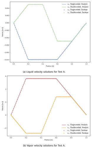
where $A_v=\frac{\pi }{4}{D}_{\mathrm{w}\mathrm{i}\mathrm{c}\mathrm{k},\mathrm{i}}^2$ is the vapor flow cross-sectional area, and $A_{\mathrm{\ell }}=A-A_v$ is the liquid flow cross-sectional area. Velocities for both the single-ended and double-ended configurations are shown in Fig. 8 and compared with the analytical solutions given in Eq. (55(55) $u_v(x)=\frac{\underset{0}{\overset{x}{\int }}q{ }^{\mathrm{\prime }}(x{ }^{\mathrm{\prime }})\mathrm{d}x{ }^{\mathrm{\prime }}}{{\rho }_v{h}_{\mathrm{\ell }v}{A}_v},u_{\mathrm{\ell }}(x)=-\frac{\underset{0}{\overset{x}{\int }}q{ }^{\mathrm{\prime }}(x{ }^{\mathrm{\prime }})\mathrm{d}x{ }^{\mathrm{\prime }}}{{\rho }_{\mathrm{\ell }}{h}_{\mathrm{\ell }v}{A}_{\mathrm{\ell }}},$(55) ), showing excellent agreement. With uniform heating and cooling, the velocities change linearly, in accordance with Eq. (55)(55) $u_v(x)=\frac{\underset{0}{\overset{x}{\int }}q{ }^{\mathrm{\prime }}(x{ }^{\mathrm{\prime }})\mathrm{d}x{ }^{\mathrm{\prime }}}{{\rho }_v{h}_{\mathrm{\ell }v}{A}_v},u_{\mathrm{\ell }}(x)=-\frac{\underset{0}{\overset{x}{\int }}q{ }^{\mathrm{\prime }}(x{ }^{\mathrm{\prime }})\mathrm{d}x{ }^{\mathrm{\prime }}}{{\rho }_{\mathrm{\ell }}{h}_{\mathrm{\ell }v}{A}_{\mathrm{\ell }}},$(55) . For the double-ended configuration, the total mass flow rate required for the given power transmission is split between two ends; thus the maximum speed of either phase is cut by a factor of 2. The decreased average speed of the double-ended configuration implies a lower pressure drop, since frictional terms in both phases are proportional to speed.

Fig. 8. Velocity solutions for test A

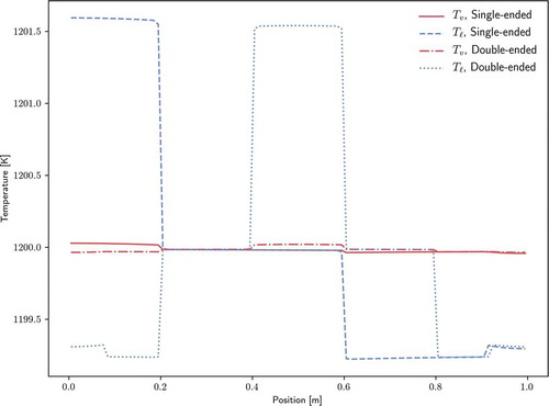
Figure 9 shows the liquid and vapor temperature profiles for both configurations. For both cases, the temperature varies less than 3 K over the length of the heat pipe. Because zero net power is added to the heat pipe over the course of the transient, the energy remains constant and is only redistributed; thus, the final temperatures are very close to the initial temperature of 1200 K. Since heating and cooling are applied to the liquid phase, the liquid phase temperature exceeds the vapor phase in the evaporator and is lower than the vapor phase in the condenser.

Fig. 9. Temperature solutions for test A

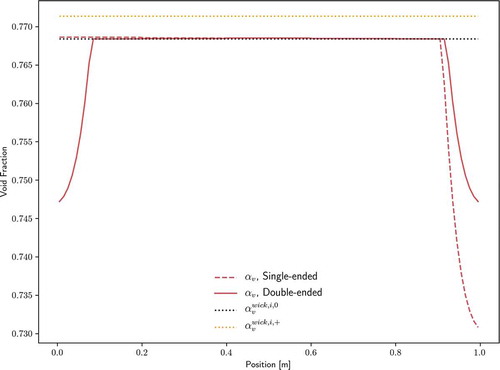
The void fraction profile is shown in Fig. 10. Recall from Sec. II.A.1 that ${\alpha }_v^{\mathrm{w}\mathrm{i}\mathrm{c}\mathrm{k},\mathrm{i},0}$ corresponds to the liquid-vapor interface flat at the inner surface of the wick, and ${\alpha }_v^{\mathrm{w}\mathrm{i}\mathrm{c}\mathrm{k},\mathrm{i},+}$ corresponds to full curvature inward at the inner surface of the wick. Therefore, for both configurations, the liquid-vapor interface is only slightly curved for most of the heat pipe length with some minor pooling of the liquid at the condenser end(s). In this case, the steady-state temperature distribution is nearly identical to the initial temperature, at which the volume of working fluid was determined with the fully saturated wick assumption. Therefore, the minor pooling is not a result of thermal expansion but rather just displacement from pore sites.

Fig. 10. Void fraction solutions for test A

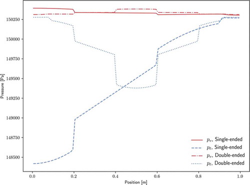
The pressure distributions of both phases are shown for both configurations in Fig. 11. For both configurations, the liquid pressure drop is dominant to the vapor pressure drop. Wet points (where liquid and vapor pressure are approximately equal) appear at the end of the condenser section(s). In the case of the double-ended configuration, the liquid and vapor flow paths are decreased by a factor of 2 over the single-ended configuration, thus leading to significantly smaller pressure drops.

Fig. 11. Pressure solutions for test A

Pressure solutions are compared against analytical pressure drop relations for the single-ended configuration. For the vapor phase, the theory of Cotter⁴⁰ is used. The radial Reynolds number for the vapor phase,

(56) $\mathrm{R}{\mathrm{e}}_{r,v}\equiv \frac{{\rho }_v{w}_v{R}_v}{{\mu }_v}=\frac{1}{2\pi {\mu }_v}\frac{\mathrm{d}{\dot{m}}_v}{\mathrm{d}x},$(56)

where $w_v$ is the radial vapor velocity component and $R_v=\frac{1}{2}{D}_{\mathrm{w}\mathrm{i}\mathrm{c}\mathrm{k},\mathrm{i}}$, is used to distinguish between pressure drop formulations. The maximum radial Reynolds number for this test problem was determined to be approximately 11.7, which Cotter’s theory classifies as “turbulent,” leading to the following pressure drop²:

(57a) $\frac{\mathrm{d}{p}_v}{\mathrm{d}x}=-\frac{s(x){\dot{m}}_v(x)}{4{\rho }_v{R}_v^4}\frac{\mathrm{d}{\dot{m}}_v}{\mathrm{d}x}-\frac{8a(x){\mu }_v{\dot{m}}_v(x)}{{\rho }_v\pi R_v^4},$(57a)

(57b) $s(x)=\left\{\begin{array}{cc}1& q(x)>0\\ 0& q(x)=0\\ \frac{4}{{\pi }^2}& q(x)<0\\ \hspace{0.17em}& \hspace{0.17em}\end{array}\right.,$(57b)

and

(57c) $a(x)=\left\{\begin{array}{cc}1& q(x)=0\\ 0& q(x)\ne 0\hspace{0.17em}\hspace{0.17em}\end{array}\right..$(57c)

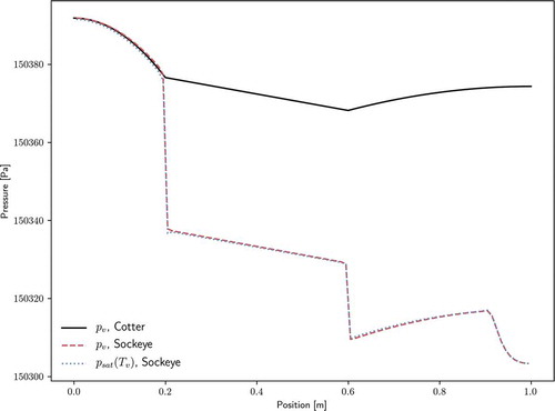
Figure 12 shows the comparison of this analytic solution with the pressure solution from Sockeye, as well as the saturation pressure at the vapor temperature. Vapor pressure drops within each region (evaporator, adiabatic, and condenser) match analytical solutions very well. However, Sockeye results indicate pressure drops between these regions that are not shown by the analytic models. Note from the pressure scale that these jumps are actually quite small, on the order of 10 Pa. As for the cause of these jumps, there is strong agreement between Sockeye’s pressure curve and saturation pressure curve, which indicates that the vapor phase is nearly following the saturation condition. The saturation pressure profile suggests the reason for these pressure drops: the temperature changes sharply at these locations. The analytic solution does not consider the nonisothermal effects.

Fig. 12. Comparison of vapor pressure drop with analytic solution for test A

For the liquid phase, Darcy’s law is used to analyze the pressure drop²:

(58) $\frac{\mathrm{d}{p}_{\mathrm{\ell }}}{\mathrm{d}x}=-\frac{{\mu }_{\mathrm{\ell }}{u}_{\mathrm{\ell }}}{K}\frac{A_{\mathrm{w}\mathrm{i}\mathrm{c}\mathrm{k},\mathrm{\ell }}}{{\alpha }_{\mathrm{\ell }}A},$(58)

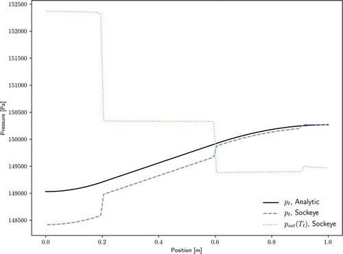
where the factor $A_{\mathrm{w}\mathrm{i}\mathrm{c}\mathrm{k},\mathrm{\ell }}/({\alpha }_{\mathrm{\ell }}A)$ is applied because only a fraction of the liquid channel is through the porous structure. Fig. 13 shows a comparison of this analytic solution with Sockeye's liquid pressure solution, as well as the saturation pressure at the liquid temperature. Again, pressure drops within each region match very well to the analytic solution, but pressure drops between regions are significant. Unlike the vapor phase, the liquid phase does not follow the saturation curve, but temperature jumps are present in the phase that do have an impact on the pressure profile.

Fig. 13. Comparison of liquid pressure drop with analytic solution for test A

V.B. Test B: SAFE-30 Heat Pipe Module Test

For this test problem, the SAFE-30 heat pipe module experiment⁷ described in Sec. IV is modeled. For this simulation, the 1-D, two-phase flow channel is coupled to heat conduction in the heat pipe cladding, which demonstrates the ability to account for the thermal resistance of the heat pipe and the transient effects of the cladding’s thermal capacity. This experiment started from room temperature, so the sodium working fluid was initially frozen, but Sockeye is not yet equipped to model startup, so the simulation was started from $t=8000$ s. The experiment was run until t = 25 200 s (7 h), but the Sockeye simulation results shown here are at $t=9575$ s because failure occurs shortly afterward; this failure is discussed later in this section.

Table III summarizes the heat pipe design used in this simulation, which is taken or derived from the experiment, with the exception of the permeability, which was not reported in Ref. 7. The experiment estimated the power input to the evaporator from the “fuel tubes” based on a lumped energy balance and measured thermocouple values. This power is denoted by “${\dot{Q}}_{\mathrm{e}\mathrm{v}\mathrm{a}\mathrm{p},\mathrm{F}\mathrm{T}}$, Experiment” in Fig. 14. This estimated power input was used as the input power to the evaporator in the Sockeye simulation by linearly interpolating between experimental points, which is denoted by “${\dot{Q}}_{\mathrm{e}\mathrm{v}\mathrm{a}\mathrm{p},\mathrm{F}\mathrm{T}}$, Sockeye.” Also in Fig. 14 is the experimental estimation of the radiative power from the condenser region and exposed evaporator region, denoted by “$-{\dot{Q}}_{\mathrm{r}\mathrm{a}\mathrm{d},\mathrm{n}\mathrm{o}\mathrm{n}\mathrm{p}\mathrm{o}\mathrm{o}\mathrm{l}}$, Experiment”; as Reid notes, this does not account for the radiative losses from the condenser pool since there were no thermocouples in that region. For the Sockeye simulation, radiative boundary conditions, as described in Table I, were used. In the experiment, the condenser section is fully exposed (thus having a view factor of $F=1$), but the evaporator section is only partially exposed due to contact with the fuel tubes, and a view factor of $F=0.25$ is used here. The environment temperature for the radiation exchange and surface emissivity were given from Ref. 7 to be 296 K and 0.4, respectively. For this demonstration, the evaporator and condenser regions were discretized into 50 elements each, and BDF2 time integration with an adaptive time step size was used.

TABLE III Test B Heat Pipe Description

Parameter	Value
Working fluid	Sodium
Working fluid mass, $m$	0.1453 kg
Wick inner diameter, $D_{\mathrm{w}\mathrm{i}\mathrm{c}\mathrm{k},\mathrm{i}}$	0.0174 m
Wick outer diameter, $D_{\mathrm{w}\mathrm{i}\mathrm{c}\mathrm{k},\mathrm{o}}$	0.0207 m
Cladding inner diameter, $D_{\mathrm{c}\mathrm{l}\mathrm{a}\mathrm{d},\mathrm{i}}$	0.0221 m
Cladding outer diameter, $D_{\mathrm{c}\mathrm{l}\mathrm{a}\mathrm{d},\mathrm{o}}$	0.0254 m
Evaporator length, $L_{\mathrm{e}\mathrm{v}\mathrm{a}\mathrm{p}}$	0.43 m
Condenser length, $L_{\mathrm{c}\mathrm{o}\mathrm{n}\mathrm{d}}$	0.77 m
Wick porosity, $\phi$	0.807308741
Pore radius, $R_{\mathrm{p}\mathrm{o}\mathrm{r}\mathrm{e}}$	47 $\times {10}^{-6}$ m
Wick permeability, $K$	10${ }^{-10}$ m${ }^2$
Orientation	Horizontal

Fig. 14. Comparison of experimental and numerical power transients for test B

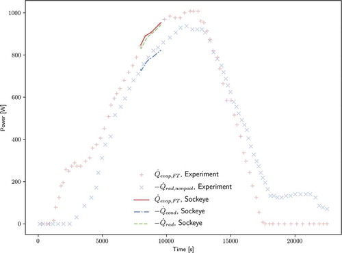
Figure 14 shows, in addition to experimental power estimations and Sockeye input, the resulting Sockeye radiative power losses in the condenser and evaporator sections. The set “$-{\dot{Q}}_{\mathrm{c}\mathrm{o}\mathrm{n}\mathrm{d}}$, Sockeye” shows the radiation power of the entire condenser section, including the liquid pool, and “$-{\dot{Q}}_{\mathrm{r}\mathrm{a}\mathrm{d}}$, Sockeye” additionally includes the radiation power of the exposed evaporator section. Unfortunately, neither of these have a direct experimental comparison (experimental results include evaporator but not condenser pool), but it is at least useful to verify that the total radiative power is roughly following the input power.

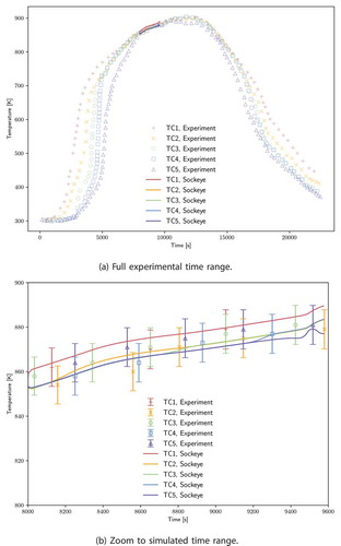
Figure 15a shows the temperature transient for the five thermocouples installed on the heat pipe. These thermocouple locations are given in Table IV. Figure 15b shows a zoom view for the simulated time period with error bars for the experimental data points. For Type C thermocouples, the error limits are the greater of 4.5°C for temperatures up to 425°C and 1% for temperatures up to 2320°C (Ref. 41); thus, the error bars in the considered temperature range correspond to 1%. The Sockeye solution stays within all of these error bars. Both the power and temperature transients are strongly dependent on the modeling of boundary conditions on the cladding as well as the total thermal capacity of the heat pipe. Future work is planned to improve upon the simulation setup used here by not using experimental estimations for evaporator power input, but instead using the input electric power to the heat cartridges and then performing lumped radiation transfer between heat cartridges, fuel tubes, the heat pipe, and the environment, similar to what is done in Ref. 6.

TABLE IV SAFE-30 Thermocouple Locations

Name	Distance from Evaporator Endcap
TC1	0.216 m
TC2	0.508 m
TC3	0.711 m
TC4	0.914 m
TC5	1.09 m

Fig. 15. Comparison of experimental thermocouple values against temperature solution values at thermocouple positions for test B

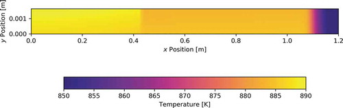
Figure 16 shows the temperature profiles at the final time, and it can be seen that the heat pipe operates nearly isothermally except for the liquid condenser pool, which attains a much lower temperature because its only source of heat is through condensation at its axial surface, while liquid in the rest of the heat pipe has a much greater surface-to-volume ratio. Figure 17 shows the final temperature profile in the heat pipe cladding, with the bottom edge corresponding to the inner cladding surface. The scale’s lower bound was increased to exclude some of the lower temperatures in the pool region to give the radial temperature gradient more visibility.

Fig. 16. Final temperature profiles for test B

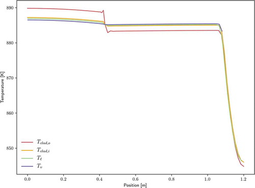
Fig. 17. Final cladding temperature profile for test B

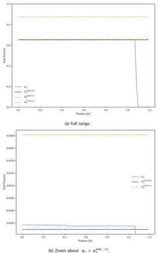
Figures 18a and 18b show a full view and zoom view, respectively, of the computed void fraction profile. The full view shows that for most of the heat pipe, the liquid-vapor interface is near the inner surface of the wick, and the zoom view shows that the interface is nearly flat. Figure 18a shows that in the final 10 cm, a liquid condenser pool (${\alpha }_v\approx 0$) formed. The formation of this liquid condenser pool is the reason for the simulation failure shortly after $t=9575$ s. Sockeye currently is not numerically robust in the limit ${\alpha }_v\to 0$; phase disappearance treatment is a high-priority item of future work. Heat pipes are commonly designed with more fluid than the annulus and wick can accommodate at a typical operating temperature, and this excess liquid volume grows with thermal expansion.

Fig. 18. Final void fraction solutions for test B

Last, the final solutions for velocity and pressure are presented. Velocity profiles are shown in Fig. 19 and follow the trends suggested by Eq. 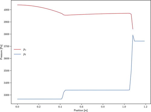(55)(55) $u_v(x)=\frac{\underset{0}{\overset{x}{\int }}q{ }^{\mathrm{\prime }}(x{ }^{\mathrm{\prime }})\mathrm{d}x{ }^{\mathrm{\prime }}}{{\rho }_v{h}_{\mathrm{\ell }v}{A}_v},u_{\mathrm{\ell }}(x)=-\frac{\underset{0}{\overset{x}{\int }}q{ }^{\mathrm{\prime }}(x{ }^{\mathrm{\prime }})\mathrm{d}x{ }^{\mathrm{\prime }}}{{\rho }_{\mathrm{\ell }}{h}_{\mathrm{\ell }v}{A}_{\mathrm{\ell }}},$(55) ; i.e., the vapor velocity increases where there is heating and decreases where there is cooling, with liquid velocity doing the opposite. In this case, there is a condenser pool, so the liquid velocity is zero in this region. Note that vapor solutions are not plotted where no vapor exists. The pressure profiles are shown in Fig. 20. The vapor pressure features a drop over the evaporator region due to acceleration and gradual pressure recovery in the condenser; however, unlike for test A, there is no sharp pressure drop between the evaporator and condenser. This is due to a much more gradual temperature drop between the regions, which is owed to the intermediate cladding layer and solution-dependent condenser boundary conditions, both not present in test A. The liquid pressure profile does show a significant pressure drop between the condenser and evaporator since the liquid phase has a sharper temperature gradient there. The liquid pressure drop due to porous losses is small in comparison.

Fig. 19. Final velocity solutions for test B

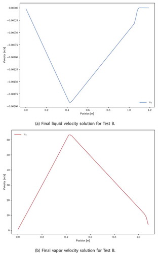
Fig. 20. Final pressure solutions for test B

V.C. Test C: Spatial Convergence Verification

To verify theoretical spatial convergence rates, the Method of Manufactured Solutions (MMS) was used. To simplify the problem, the following assumptions were used:

1. constant volume fraction

2. zero interfacial heat transfer coefficients

3. zero pressure relaxation

4. zero heat conduction

5. infinite permeability

6. zero gravity

7. zero wall friction

8. zero wall heat.

With the first three assumptions, the liquid and vapor phases are effectively decoupled, and with the remaining assumptions, Eqs. (5)(5) $\frac{\mathrm{\partial }{\alpha }_{\mathrm{\ell }}A}{\mathrm{\partial }t}+u_{\mathrm{i}\mathrm{n}\mathrm{t}}\frac{\mathrm{\partial }{\alpha }_{\mathrm{\ell }}}{\mathrm{\partial }x}A=\mathrm{\Theta }\left(p_{\mathrm{\ell }}+\mathrm{\Delta }{p}_{\mathrm{c}\mathrm{a}\mathrm{p}}-p_v\right)A-\frac{{\mathrm{\Gamma }}_{\mathrm{i}\mathrm{n}\mathrm{t}}{a}_{\mathrm{i}\mathrm{n}\mathrm{t}}A}{{\rho }_{\mathrm{i}\mathrm{n}\mathrm{t}}},$(5) through (11(11) $\begin{array}{rl}& \frac{\mathrm{\partial }{\alpha }_v{\rho }_v{E}_{v}A}{\mathrm{\partial }t}+\frac{\mathrm{\partial }{\alpha }_v{u}_v\left({\rho }_v{E}_v+p_v\right)A}{\mathrm{\partial }x}=p_{\mathrm{i}\mathrm{n}\mathrm{t}}{u}_{\mathrm{i}\mathrm{n}\mathrm{t}}\frac{\mathrm{\partial }{\alpha }_v}{\mathrm{\partial }x}A\\ & +{\bar{p}}_{\mathrm{i}\mathrm{n}\mathrm{t}}\mathrm{\Theta }\left(p_{\mathrm{\ell }}+\mathrm{\Delta }{p}_{\mathrm{c}\mathrm{a}\mathrm{p}}-p_v\right)A+{\alpha }_v{\rho }_v{g}_x{u}_{v}A\\ & +q_v^{\mathrm{w}\mathrm{a}\mathrm{l}\mathrm{l}}{P}_{\mathrm{w}\mathrm{a}\mathrm{l}\mathrm{l}}+q_v^{\mathrm{i}\mathrm{n}\mathrm{t}}{a}_{\mathrm{i}\mathrm{n}\mathrm{t}}A+{\mathrm{\Gamma }}_{\mathrm{i}\mathrm{n}\mathrm{t}}{E}_v^{\mathrm{i}\mathrm{n}\mathrm{t}}{a}_{\mathrm{i}\mathrm{n}\mathrm{t}}A.\end{array}$(11) ) reduce to a homogeneous system, to which MMS sources are added, resulting in the following system:

(59) $\frac{\mathrm{\partial }{\alpha }_{\mathrm{\ell }}{\rho }_{\mathrm{\ell }}A}{\mathrm{\partial }t}+\frac{\mathrm{\partial }{\alpha }_{\mathrm{\ell }}{\rho }_{\mathrm{\ell }}{u}_{\mathrm{\ell }}A}{\mathrm{\partial }x}=S_{{\alpha }_{\mathrm{\ell }}{\rho }_{\mathrm{\ell }}A},$(59)

(60) $\frac{\mathrm{\partial }{\alpha }_{\mathrm{\ell }}{\rho }_{\mathrm{\ell }}{u}_{\mathrm{\ell }}A}{\mathrm{\partial }t}+\frac{\mathrm{\partial }{\alpha }_{\mathrm{\ell }}\left({\rho }_{\mathrm{\ell }}{u}_{\mathrm{\ell }}^2+p_{\mathrm{\ell }}\right)A}{\mathrm{\partial }x}=S_{{\alpha }_{\mathrm{\ell }}{\rho }_{\mathrm{\ell }}{u}_{\mathrm{\ell }}A},$(60)

(61) $\frac{\mathrm{\partial }{\alpha }_{\mathrm{\ell }}{\rho }_{\mathrm{\ell }}{E}_{\mathrm{\ell }}A}{\mathrm{\partial }t}+\frac{\mathrm{\partial }{\alpha }_{\mathrm{\ell }}{u}_{\mathrm{\ell }}\left({\rho }_{\mathrm{\ell }}{E}_{\mathrm{\ell }}+p_{\mathrm{\ell }}\right)A}{\mathrm{\partial }x}=S_{{\alpha }_{\mathrm{\ell }}{\rho }_{\mathrm{\ell }}{E}_{\mathrm{\ell }}A},$(61)

(62) $\frac{\mathrm{\partial }{\alpha }_v{\rho }_{v}A}{\mathrm{\partial }t}+\frac{\mathrm{\partial }{\alpha }_v{\rho }_v{u}_{v}A}{\mathrm{\partial }x}=S_{{\alpha }_v{\rho }_{v}A},$(62)

(63) $\frac{\mathrm{\partial }{\alpha }_v{\rho }_v{u}_{v}A}{\mathrm{\partial }t}+\frac{\mathrm{\partial }{\alpha }_v\left({\rho }_v{u}_v^2+p_v\right)A}{\mathrm{\partial }x}=S_{{\alpha }_v{\rho }_v{u}_{v}A},$(63)

and

(64) $\frac{\mathrm{\partial }{\alpha }_v{\rho }_v{E}_{v}A}{\mathrm{\partial }t}+\frac{\mathrm{\partial }{\alpha }_v{u}_v\left({\rho }_v{E}_v+p_v\right)A}{\mathrm{\partial }x}=S_{{\alpha }_v{\rho }_v{E}_{v}A},$(64)

where $S_i$ represents the MMS source rate for $i$.

To facilitate the MMS source derivation, the ideal gas equation of state is used for both phases, with different parameters:

(65) $p_k(\rho ,e)=\rho e({\gamma }_k-1),$(65)

where ${\gamma }_{\mathrm{\ell }}=2$ and ${\gamma }_v=1.4$.

The chosen MMS solutions are the following:

(66) ${\alpha }_k(x,t)=0.5,$(66)

(67) ${\rho }_k(x,t)=A_k(sin(B_{k}x+C_{k}t)+2),$(67)

(68) $u_k(x,t)=A_{k}tsin(\pi x),$(68)

and

(69) $p_k(x,t)=A_k(cos(B_{k}x+C_{k}t)+2),$(69)

where $A_k$, $B_k$, and $C_k$ are chosen constants for phase $k$. The chosen constants were $A_{\mathrm{\ell }}=B_{\mathrm{\ell }}=C_{\mathrm{\ell }}=1$ and $A_v=B_v=C_v=0.5$.

Runs were performed on the domain $x\in (0,1)$ with a cross-sectional area of $A=1$. To prevent temporal error from obscuring spatial error, a small time step size of $\mathrm{\Delta }t={10}^{-6}$ s was used with the third-order, explicit, strong-stability-preserving temporal integration scheme.⁴² Ten time steps were used in each of the five runs of different mesh sizes, with the coarsest mesh size being 0.1 m and refining the mesh by a factor of 2 for each subsequent run. Error was computed for density, velocity, and pressure in each phase. The following error norm was used to assess convergence for a quantity $y$:

(70) $\parallel y-y_h{\parallel }_1\equiv \sum _i{h}_i|y(x_i)-Y_i|,$(70)

where in this context,

$h$ =	=	mesh size, i.e., $\mathrm{\Delta }x$
$y_h$ =	=	approximate solution of the exact solution $y$
$i$ =	=	an element index
$Y_i$ =	=	associated solution value.

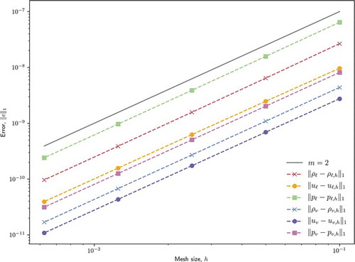
Without slope reconstruction, the spatial discretization is described as a Godunov scheme, which is first-order accurate, and with full slope reconstruction, second-order accuracy is expected.^32,33 Figures 21 and 22 show the results of this study for the Godunov scheme and full-reconstruction scheme, respectively. Reference slopes for first-order and second-order accuracy are provided where relevant. The Godunov scheme demonstrates the expected first-order accuracy for density and pressure but velocity encounters a second-order accuracy superconvergence for the chosen test problem and error norm. The full slope reconstruction scheme demonstrates universal second-order accuracy in the chosen error norm.

Fig. 21. Spatial convergence for the Godunov scheme

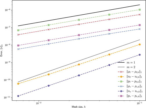
Fig. 22. Spatial convergence for the full-reconstruction scheme

VI. CONCLUSIONS

Sockeye provides a versatile tool for performing transient simulations of conventional axial heat pipes. Two-phase flow simulation is provided by the application of specialized closures to the nonequilibrium seven-equation model,^24–26,34 a well-posed 1-D model of two-phase flow. This can then be coupled to heat conduction in the heat pipe cladding to account for thermal capacity and resistance due to the cladding. Capillary driving forces are captured through the use of a geometric mapping function of capillary pressure to volume fraction, and the corresponding capillary pressure driving force is achieved through the use of pressure relaxation terms. A selection of heat pipe operational limits is inherent in the model, such as the capillary limit, viscous limit, and sonic limit, but their demonstration is planned for future work.

Comparisons were made against analytical velocity solutions and pressure drop relations. Velocity solutions had excellent agreement with analytic solutions, and pressure drops matched well within each axial region but with significant pressure drops between regions due to large temperature gradients at these locations. Sockeye was also compared against experimental data from the SAFE-30 heat pipe module test, but the formation of a condenser pool caused a simulation failure because Sockeye is not yet robust in the phase disappearance limits. For the duration of the experiment simulated, temperature solutions stayed within thermocouple error limits.

Future work for Sockeye includes a number of high-priority items for use as a practical engineering tool. Robustness in the phase disappearance limit is targeted, which entails appropriate guarding against division by zero-valued volume fractions and smooth transitions to single-phase equations. This is important because many heat pipes are designed with excess working fluid and thus will form condenser pools. A practical solution is needed for modeling the startup process, and the presence of noncondensable gases needs to be considered. Other work includes demonstration of relevant operational limits and further validation and verification efforts.

Acknowledgments

The Sockeye and RELAP-7 nuclear reactor system analysis code developments are being carried out under the auspices of Idaho National Laboratory, a contractor of the U.S. Government under contract number DEAC07-05ID14517. Accordingly, the U.S. Government retains a nonexclusive, royalty-free license to publish or reproduce the published form of this contribution, or allows others to do so, for U.S. Government purposes.

References

- D. A. REAY, P. A. KEW, and R. J. McGLEN, Heat Pipes: Theory, Design and Applications, Elsevier Ltd (2014).
- A. FAGHRI, Heat Pipe Science and Technology, Global Digital Press (2016).
- C. J. PERMANN et al., “MOOSE: Enabling Massively Parallel Multiphysics Simulation,” SoftwareX, 11, 100430 (2020); https://doi.org/10.1016/j.softx.2020.100430.
- C. MATTHEWS et al., “Coupled Multiphysics Simulations of Heat Pipe Microreactors Using DireWolf,” Nucl. Technol., 207, 1142 (2021); https://doi.org/10.1080/00295450.2021.1906474.
- A. FAGHRI and C. HARLEY, “Transient Lumped Heat Pipe Analyses,” Heat Recovery Syst. CHP, 14, 4, 351 (1994); https://doi.org/10.1016/0890-4332(94)90039-6.
- R. S. REID, “Heat Pipe Transient Response Approximation,” LA-UR-01-5895, Los Alamos National Laboratory (2002).
- R. S. REID, J. T. SENA, and A. L. MARTINEZ, “Sodium Heat Pipe Module Test for the SAFE-30 Reactor Prototype,” AIP Conf. Proc., 552, 869 (2001); https://doi.org/10.1063/1.1358021.
- Z. ZUO and A. FAGHRI, “A Network Thermodynamic Analysis of the Heat Pipe,” Int. J. Heat Mass Transfer, 41, 11, 1473 (1998); https://doi.org/10.1016/S0017-9310(97)00220-2.
- H. SHABGARD et al., “Heat Pipe Heat Exchangers and Heat Sinks: Opportunities, Challenges, Applications, Analysis, and State of the Art,” Int. J. Heat Mass Transfer, 89, 138 (2015); https://doi.org/10.1016/j.ijheatmasstransfer.2015.05.020.
- S. BENN et al., “Analysis of Thermosyphon/Heat Pipe Integration for Feasibility of Dry Cooling for Thermoelectric Power Generation,” Appl. Thermal Eng., 104, 358 (2016); https://doi.org/10.1016/j.applthermaleng.2016.05.045.
- L. M. POPLASKI, A. FAGHRI, and T. L. BERGMAN, “Analysis of Internal and External Thermal Resistances of Heat Pipes Including Fins Using a Three-Dimensional Numerical Simulation,” Int. J. Heat Mass Transfer, 102, 455 (2016); https://doi.org/10.1016/j.ijheatmasstransfer.2016.05.116.
- K. PANDA, I. DULERA, and A. BASAK, “Numerical Simulation of High Temperature Sodium Heat Pipe for Passive Heat Removal in Nuclear Reactors,” Nucl. Eng. Des., 323, 376 (2017); https://doi.org/10.1016/j.nucengdes.2017.03.023.
- M. MA et al., “A Pure-Conduction Transient Model for Heat Pipes via Derivation of a Pseudo Wick Thermal Conductivity,” Int. J. Heat Mass Transfer, 149, 119122 (2020); https://doi.org/10.1016/j.ijheatmasstransfer.2019.119122.
- W. J. BOWMAN and J. E. HITCHCOCK, “Transient, Compressible Heat-Pipe Vapor Dynamics,” presented at the ASME 1988 Natl. Heat Transfer Conf., Houston, Texas, July 24–27, 1988, 1, 329 (1988).
- Y. CAO and A. FAGHRI, “Transient Two-Dimensional Compressible Analysis for High-Temperature Heat Pipes with Pulsed Heat Input,” Numer. Heat Transfer Part A, 18, 4, 483 (1990); https://doi.org/10.1080/10407789008944804.
- V. H. RANSOM and H. CHOW, “ATHENA Heat Pipe Transient Model,” Space Nucl. Power Syst., 389 (1987).
- M. J. HALL and J. M. DOSTER, “A Sensitivity Study of the Effects of Evaporation/Condensation Accommodation Coefficients on Transient Heat Pipe Modeling,” Int. J. Heat Mass Transfer, 33, 3, 465 (1990); https://doi.org/10.1016/0017-9310(90)90182-T.
- J.-M. TOURNIER and M. S. EL-GENK, “A Heat Pipe Transient Analysis Model,” Int. J. Heat Mass Transfer, 37, 4, 753 (1994); https://doi.org/10.1016/0017-9310(94)90113-9.
- Y. CAO and A. FAGHRI, “A Numerical Analysis of High-Temperature Heat Pipe Startup from the Frozen State,” J. Heat Transfer, 115, 247 (1993); https://doi.org/10.1115/1.2910657.
- M. R. BAER and J. W. NUNZIATO, “A Theory of Deflagration-to-Detonation Transition (DDT) in Granular Explosives,” Int. J. Multiphase Flow, 12, 6, 861 (1986); https://doi.org/10.1016/0301-9322(86)90033-9.
- R. SAUREL and R. ABGRALL, “A Multiphase Godunov Method for Compressible Multifluid and Multiphase Flows,” J. Comput. Phys., 150, 2, 425 (1999); https://doi.org/10.1006/jcph.1999.6187.
- S. TOKAREVA and E. TORO, “HLLC-Type Riemann Solver for the Baer–Nunziato Equations of Compressible Two-Phase Flow,” J. Comput. Phys., 229, 10, 3573 (2010); https://doi.org/10.1016/j.jcp.2010.01.016.
- A. AMBROSO, C. CHALONS, and P.-A. RAVIART, “A Godunov-Type Method for the Seven-Equation Model of Compressible Two-phase Flow,” Comput. Fluids, 54, 67, 67 (2012); https://doi.org/10.1016/j.compfluid.2011.10.004.
- R. A. BERRY et al., “RELAP-7 Theory Manual,” INL/EXT-14-31366 Revision 3, Idaho National Laboratory (2018).
- R. A. BERRY et al., “Sockeye Heat Pipe Code Theory Development: Based on the 7-Equation, Two-Phase Flow Model of RELAP-7,” presented at the Int. Topl. Mtg. Advances in Thermal Hydraulics (ATH’20), October 20-23, 2020, Electricité de France Lab Paris-Saclay, France (2020).
- R. A. BERRY, R. SAUREL, and O. LEMETAYER, “The Discrete Equation Method (DEM) for Fully Compressible, Two-Phase Flows in Ducts of Spatially Varying Cross-Section,” Nucl. Eng. Des., 240, 11, 3797 (2010); https://doi.org/10.1016/j.nucengdes.2010.08.003.
- A. CHINNAYYA, E. DANIEL, and R. SAUREL, “Modelling Detonation Waves in Heterogeneous Energetic Materials,” J. Comput. Phys., 196, 2, 490 (2004); https://doi.org/10.1016/j.jcp.2003.11.015.
- S. D. GUPTA, “Experimental High Temperature Coefficients of Compressibility and Expansivity of Liquid Sodium and Other Related Properties,” PhD Thesis, Columbia University (1977).
- G. H. GOLDEN and J. V. TOKAR, “Thermophysical Properties of Sodium,” ANL-7323, Argonne National Laboratory (1967).
- O. J. FOUST, Sodium-NaK Engineering Handbook. Volume I. Sodium Chemistry and Physical Properties, Gordon and Breach, Science Publishers, Inc (1972).
- A. D. PASTERNAK, “Isothermal Compressibility of the Liquid Alkali Metals,” Mater. Sci. Eng., 3, 2, 65 (1968); https://doi.org/10.1016/0025-5416(68)90019-0.
- E. TORO, Riemann Solvers and Numerical Methods for Fluid Dynamics: A Practical Introduction, Springer, Berlin (2009).
- R. LEVEQUE and D. CRIGHTON, Finite Volume Methods for Hyperbolic Problems, Cambridge Texts in Applied Mathematics, Cambridge University Press (2002).
- D. FURFARO and R. SAUREL, “A Simple HLLC-Type Riemann Solver for Compressible Nonequilibrium Two-Phase Flows,” Comput. Fluids, 111, 159 (2015); https://doi.org/10.1016/j.compfluid.2015.01.016.
- C. F. CURTISS and J. O. HIRSCHFELDER, “Integration of Stiff Equations,” Proc. Natl. Acad. Sci., 38, 3, 235 (1952); https://doi.org/10.1073/pnas.38.3.235.
- A. FAGHRI, M. BUCHKO, and Y. CAO, “A Study of High-Temperature Heat Pipes with Multiple Heat Sources and Sinks: Part I—Experimental Methodology and Frozen Startup Profiles,” J. Heat Transfer, 113, 4, 1003 (1991); https://doi.org/10.1115/1.2911193.
- A. FAGHRI, M. BUCHKO, and Y. CAO, “A Study of High-Temperature Heat Pipes with Multiple Heat Sources and Sinks: Part II—Analysis of Continuum Transient and Steady-State Experimental Data with Numerical Predictions,” J. Heat Transfer, 113, 4, 1010 (1991); https://doi.org/10.1115/1.2911194.
- S. LEE, “NEUP Project 20-19735: Experiments for Modeling and Validation of Liquid-Metal Heat Pipe Simulation Tools for Micro-Reactors,” Technical Abstract, U.S. Department of Energy (2020).
- V. PETROV, “NEUP Project 19-17416: Experiments and Computations to Address the Safety Case of Heat Pipe Failures in Special Purpose Reactors,” Technical Abstract, U.S. Department of Energy (2019).
- T. COTTER, “Theory of Heat Pipes,” LA-3246-MS, Los Alamos National Laboratory (1965).
- G. W. BURNS et al., “Temperature-Electromotive Force Reference Functions and Tables for the Letter-Designated Thermocouple Types Based on the ITS-90,” Monograph 175, National Institute of Standards and Technology (1993).
- S. GOTTLIEB, “On High Order Strong Stability Preserving Runge-Kutta and Multi Step Time Discretizations,” J. Sci. Comput., 25, 1/2 (2005); https://doi.org/10.1007/s10915-004-4635-5.