Grizzly and BlackBear: Structural Component Aging Simulation Codes

Abstract

The operating environment of nuclear reactors imposes extreme challenges on the materials from which the structures within and surrounding the reactor are constructed. Understanding the effects of exposure to this environment is critical for ensuring the safe long-term operation of these reactors. The Grizzly and BlackBear codes are being developed to model the progression of aging mechanisms and their effects on the integrity of critical structures. These codes take advantage of the capabilities of the MOOSE framework to solve the wide range of coupled physics problems that are encountered in predictive simulation of structural degradation. This paper provides an overview of these codes, with a specific focus on two capabilities relevant for light water reactor applications: reactor pressure vessel embrittlement and concrete degradation.

Keywords:

• Structural components
• reactor pressure vessel
• concrete

I. INTRODUCTION

The structural components that comprise nuclear reactors and their supporting structures are subjected to harsh operating environments that can challenge their integrity, especially after exposure for extended durations. The aspects of nuclear power that make it attractive, such as high power density in the core, are largely responsible for these material issues. Reactor structures are subjected not only to heat flux, but also to accompanying neutron and gamma radiation emanating from the core. This is a concern both for the currently operating fleet of predominantly light water reactors (LWRs), as well as for advanced reactors currently under development.¹

In the United States, currently operating commercial reactors comprise only LWRs and provide roughly 20% of the electrical power to the grid. The aging of these reactors is a significant issue: Roughly 50% of these reactors are now operating under a 20-year extension to their original 40-year license,² and subsequent license renewals that would allow operation for an additional 20 years (i.e., up to 80 years) are being pursued by the operators of multiple plants, with the first such renewal being issued in December 2019 (Ref. 3). The U.S. Department of Energy’s (DOE’s) Light Water Reactor Sustainability (LWRS) program performs research to ensure the safe and economical long-term operation of these reactors,⁴ a significant part of which is devoted to material degradation issues.

Grizzly is a simulation code, the development of which was initiated in support of the LWRS program to simulate the aging of LWR systems, components, and structures. To understand the serviceability of an aged structure, it is important to be able to predict both the progression of the relevant aging mechanisms, as well as their effect on the ability of that structure to safely operate under anticipated service loading. Grizzly addresses both of these aspects of the aging problem. Many of the degradation phenomena of interest for nuclear structures are also observed in other civil structures. To make the simulation capabilities available to the broader scientific community and to foster collaboration, the portions of Grizzly that are not specific to nuclear applications have been released in an open-source code called BlackBear that provides a subset of Grizzly’s capabilities. The development of these codes is being led by Idaho National Laboratory (INL) in collaboration with multiple other DOE national laboratories and universities.

There is significant current interest in the development of advanced reactors, nearly all of which operate at significantly higher temperatures than LWRs and many of which include design features, such as molten salt coolants, that impose additional challenges on structural materials.^5,6 While Grizzly was originally developed exclusively for LWR applications, its scope has recently been expanded to also include modeling of structural material issues unique to advanced reactors.

Modeling the progression of aging and its effects on structural integrity almost invariably involves the solution of coupled systems of partial differential equations (PDEs) representing the individual physics involved. Grizzly and BlackBear employ the capabilities of the MOOSE framework,⁷ on which they are based, to solve these coupled PDEs using computing hardware ranging from laptops to high-performance clusters, as dictated by the problem size.

There is a very broad range of structural component degradation mechanisms of interest, especially when considering multiple reactor types. In an effort to focus research on the most pressing issues for LWRs, the U.S. Nuclear Regulatory Commission conducted an evaluation of aging issues of potential concern for operating LWRs up to 80 years, known as the expanded materials degradation assessment (EMDA), following a phenomena identification and ranking table process to identify phenomena with high importance and low knowledge. This resulted in a series of reports on major areas, which included core internals and piping, reactor pressure vessel (RPV) steel, concrete structures, and electrical cabling and insulation.

Based on the findings of the EMDA, LWR RPVs (Ref. 8) and concrete structures⁹ were chosen as the initial targets for Grizzly development. Both of these types of structures have extreme difficulty and cost associated with their replacement or repair, which means that their degradation has the potential to limit the service life of the entire nuclear power plant. Development is ongoing to address other structures, but these are the areas with the most complete capabilities currently and are the primary focus of this paper. This paper provides an overview of Grizzly’s software architecture, along with more detailed descriptions of its LWR RPV and concrete simulation capabilities, with accompanying demonstrations on each of these types of structures.

Although both the LWR RPV and concrete simulation capabilities discussed here rely heavily on structural mechanics simulation capabilities that are widely available in other codes, these are applied in ways that specifically target the needs of these applications in unique ways. Specifically, for LWR RPVs Grizzly provides an ability to perform probabilistic analysis on a population of flaws based on a three-dimensional (3-D) model of the global response of the RPV. This allows for local effects such as those demonstrated here on an analysis of a postulated cold plume region to be addressed in ways that are currently not possible with other codes. Likewise, for concrete structures, Grizzly provides an extremely flexible framework for solution of the coupled physics models essential for modeling degradation mechanisms.

II. CODE ARCHITECTURE

II.A. Multiscale Modeling

Modeling the mechanisms and effects of degradation inherently involves considering multiple length scales. Assessing the integrity of a structure subjected to degradation generally involves the use of models of entire structures or components and requires the use of models that can efficiently represent the effects of degradation on the material properties relevant at the scales of those structures. The evolution of those material properties is driven by changes in the microstructure that occur over long periods of time at the atomistic and grain scales.

In some cases, empirical models for the evolution of material properties are adequate for the purposes of engineering analysis, and Grizzly takes advantage of those models. However, such models are inherently limited to application within the parameter space in which they are calibrated. In RPVs, the primary aging concern is that the steel embrittles over time in the reactor environment and becomes more susceptible to fracture. The material property models widely used for predicting the progression of embrittlement, e.g., the model described in Ref. 10, are calibrated to data obtained from fracture tests of irradiated coupons, but the environmental exposure times of those coupons are limited to the lifetime of the current reactor fleet. Extrapolating those data to long-term operation scenarios is inherently problematic.

A major part of the Grizzly development effort has focused on developing models to predict the underlying microstructure evolution leading to RPV steel embrittlement, with the goal of developing predictive models for embrittlement over longer-term exposure to the reactor environment. This has involved the development of models at the atomistic scale^11,12 to understand mechanisms of radiation damage to the crystal structure within grains, mean-field cluster dynamics models of precipitation,¹³ crystal plasticity models to understand the effects of irradiation on flow stress behavior,^14,15 and cohesive zone model development to model temperature-dependent toughness.¹⁶

Some of these microstructure evolution models are based on continuum theories, while many of them, particularly those that represent behavior at the atomistic scale, are not. Based on continuous finite element theory, Grizzly is applicable to modeling techniques that represent continuous behavior, such as phase field, crystal plasticity, and continuum mechanics. It also can be used to solve the ordinary differential equations (ODEs) of mean-field cluster dynamics modeling. It does not, however, support techniques such as molecular dynamics and kinetic Monte Carlo that are used at atomistic scales; other codes are used for those purposes. Grizzly does provide support for reading in solutions from some of these atomistic-scale models and mapping them to continuous solution fields, which has been used for modeling precipitate nucleation in a kinetic Monte Carlo code, and then using phase-field models to predict their coarsening and growth.¹⁷

This development of predictive models of material microstructure and property evolution is extremely important and is an ongoing effort that has been proceeding in parallel with the development of tools for engineering assessment of the effect of material degradation on structural capacity. These engineering-scale tools currently use the available semi-empirical models, but as models are developed for material degradation informed by multiscale modeling, with applicability to a broader range of conditions, they will be deployed for use. The scope of the current paper is limited to the engineering-scale capabilities in Grizzly.

II.B. Relationships Between Codes

The MOOSE framework provides the foundational capabilities needed by a modern finite element–based simulation code, such as input/output, parsing, finite element data structures, solvers, parallel communication, etc. These capabilities are used to some extent by every application based on MOOSE.

A key design principle of the MOOSE framework that is carried through to all application codes based on it, is that physics models are object-oriented modular components that can be composed together in unique ways to provide an extremely wide variety of capabilities. Although the basic execution workflow can be customized to some extent, the applications built on MOOSE rely on MOOSE to drive the simulation execution process. Rather than defining their own procedural workflow, as is done with other simulation frameworks, domain-specific applications based on MOOSE implement their unique capabilities through customized modules that are plugged into the MOOSE framework and called at the appropriate times. A wide variety of systems are provided by MOOSE that provide interfaces for the most common use cases.⁷ In addition, if further customization is needed, MOOSE provides interfaces for very generic operations through the UserObject system, which is used extensively in Grizzly.

An important consequence of this modular design is that it makes sharing code between applications very straightforward. Capabilities are provided by C++ classes (or sets of such classes) that derive from base classes that define the way that they interface with the MOOSE framework. Sharing a capability with another application simply entails including directories containing the source code files that define those classes in the build process of the application that needs those capabilities.

Sharing of capabilities that are needed by multiple applications is also facilitated by the layout of the open-source MOOSE codebase, which consists of two major components: the framework and the common physics modules (or “modules”). The MOOSE modules are an area where models that provide basic sets of capabilities for a variety of physics are implemented. Application-specific specializations of these models are implemented in individual MOOSE-based applications, which include only the modules that they need.

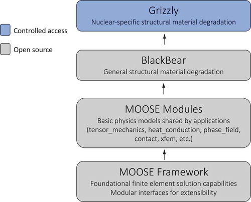
Similar to the way applications can include models from the MOOSE modules, they can also include models from other MOOSE-based applications. The designs of Grizzly and BlackBear take advantage of this. BlackBear provides a set of open-source models that are generically applicable to a variety of civil structures. The source code for BlackBear is maintained on GitHub,¹⁸ which facilitates distribution and testing and accepting code contributions from the broad research community. Grizzly inherits the full set of capabilities in BlackBear as a library, adding an additional set of models that pertain only to nuclear applications and have limitations imposed on their distribution. Thus, Grizzly is a superset of the capabilities of BlackBear, and BlackBear is a superset of the capabilities provided by the MOOSE framework and the selected MOOSE modules that it builds on, as illustrated in Fig. 1.

Fig. 1. Relationship between Grizzly, BlackBear, and the MOOSE modules and framework

II.C. Thermomechanical Solution Infrastructure

Grizzly/BlackBear simulations rely heavily on the solution of the equations of mechanical equilibrium and heat transfer, which are used to solve for the displacement $\mathit{u}$ and temperature $T$ field variables, respectively. In the absence of body forces, the equilibrium equation

(1) $\mathrm{\nabla }\cdot \sigma =\mathbf{0}$(1)

governs the mechanical deformation. The stress tensor $\sigma$ is computed from the displacement field through kinematic and constitutive relationships, shown respectively for small-strain elasticity:

(2) $\mathit{\epsilon }=\frac{1}{2}\left(\mathrm{\nabla }\mathit{u}+{(\mathrm{\nabla }\mathit{u})}^T\right)$(2)

and

(3) $\sigma =\mathbf{C}:\mathit{\epsilon },$(3)

where $\mathit{\epsilon }$ is the strain tensor, and $\mathit{C}$ is the elasticity tensor. Intrinsic strains (or eigenstrains), such as those induced by thermal expansion or swelling, are represented by subtracting them from $\mathit{\epsilon }$.

Heat transfer within a solid is governed by

(4) $\rho C_p\frac{\mathrm{\partial }T}{\mathrm{\partial }t}=k{\mathrm{\nabla }}^{2}T+\dot{Q},$(4)

where

$\rho$ =	=	density
$C_p$ =	=	specific heat at constant pressure
$k$ =	=	thermal conductivity
$\dot{Q}$ =	=	a volumetric heating rate.

The foundational capabilities to solve these mechanical equilibrium and heat equations are provided by the MOOSE tensor_mechanics and heat_conduction modules, respectively. These modules were originally developed to meet the needs of the BISON nuclear fuel performance code,¹⁹ which also relies on the solution of thermal and mechanical equations. Having these models implemented in the MOOSE modules allows Grizzly to heavily leverage the work done on these modules for BISON. For both the BISON and Grizzly applications, coupling between thermal and mechanical solutions is important, as described in Ref. 20, and MOOSE makes handling the coupling between those field variables (as well as other solution fields) straightforward.

For brevity, the mechanics [Eqs. (1)(1) $\mathrm{\nabla }\cdot \sigma =\mathbf{0}$(1) and (3(3) $\sigma =\mathbf{C}:\mathit{\epsilon },$(3) )] are shown here in their simplest form for linear elasticity. Multiple sources of nonlinearity are encountered in real-world structural degradation applications, including temperature-dependent elastic moduli, inelastic behavior due to creep or plasticity, nonlinear functions for eigenstrains, and finite deformation. Likewise, the heat [Eq. (4(4) $\rho C_p\frac{\mathrm{\partial }T}{\mathrm{\partial }t}=k{\mathrm{\nabla }}^{2}T+\dot{Q},$(4) )] can be nonlinear due to the dependence of the specific heat and conductivity on temperature. The foundational code for these equations in the MOOSE modules provides full support for handling such nonlinearities, as well as arbitrary coupling between these and other physics equations. These field equations can be solved in one dimension (spherically symmetric or axisymmetric), two dimensions (axisymmetric or Cartesian), and three dimensions (Cartesian).

II.D. Fracture Mechanics Methods

Fracture is an important failure mechanism for multiple types of structural components, so flexible fracture analysis capabilities are needed by Grizzly. The primary application for fracture capabilities in Grizzly has been RPV integrity, but it is anticipated that future research areas such as stress corrosion crack growth and graphite fracture will also require such capabilities.

To represent the jumps in the displacements or other solution fields due to fracture, Grizzly makes use of the extended finite element method^21,22 (XFEM), which allows for arbitrary discontinuities in a solution field to be represented on a finite element mesh. In XFEM, the solution field $\mathit{u}$ as a function of position $\mathit{x}$ and time $t$ is represented by a combination of the standard finite element representation of the continuous field using interpolation functions $N_I$ along with additional enrichment functions. These enrichments represent the jump across the crack with a Heaviside function $H$ and the effects of asymptotic fields near the crack tip using a set of enrichment functions $\mathrm{F}\mathrm{\_}\mathrm{L}$. The enriched field equations are expressed by

$\begin{array}{rl}& \mathit{u}(\mathit{x},t)=\underset{\mathrm{C}\mathrm{o}\mathrm{n}\mathrm{t}\mathrm{i}\mathrm{n}\mathrm{u}\mathrm{o}\mathrm{u}\mathrm{s}}{\underbrace{\sum _{I=1}^n{N}_I(\mathit{x}){\mathit{u}}_I(t)}}+\underset{\mathrm{H}\mathrm{e}\mathrm{a}\mathrm{v}\mathrm{i}\mathrm{s}\mathrm{i}\mathrm{d}\mathrm{e}\mathrm{E}\mathrm{n}\mathrm{r}\mathrm{i}\mathrm{c}\mathrm{h}\mathrm{e}\mathrm{d}}{\underbrace{\sum _{J=1}^n{N}_J(\mathit{x})H(\mathit{x}){\mathit{b}}_J(t)}}\\ & +\underset{\mathrm{N}\mathrm{e}\mathrm{a}\mathrm{r}-\mathrm{t}\mathrm{i}\mathrm{p}\mathrm{E}\mathrm{n}\mathrm{r}\mathrm{i}\mathrm{c}\mathrm{h}\mathrm{e}\mathrm{d}}{\underbrace{\sum _{K=1}^n{N}_K(\mathit{x})\sum _{L=1}^4{F}_L(\mathit{x})c_K^L(t)}},(5)\end{array}$

where

$n$ =	=	number of nodes per finite element
${\mathit{u}}_I$ =	=	nodal displacements
${\mathit{b}}_J$ =	=	additional nodal degrees of freedom corresponding to Heaviside enrichment
${\mathit{c}}_K$ =	=	additional nodal degrees of freedom corresponding to the near-tip enrichment.

Additional nodal degrees of freedom are introduced corresponding to these enrichments, which is necessary to ensure continuity of the enriched field within the material on either side of the interface.

The xfem MOOSE module provides an implementation of XFEM based on the phantom-node method,²³ which is equivalent to the original XFEM formulation with Heaviside enrichment. Details on the implementation of the xfem module, along with BISON nuclear fuel applications that motivated its development, are provided in Ref. 24. The MOOSE implementation of XFEM uses the phantom-node approach for Heaviside enrichment and provides the option to use near-tip enrichment in addition to that.

In most fracture mechanics applications, the stress intensity factors (SIFs) along the crack front are the quantity of interest. The mode-I SIF $K_I$ can be computed from the J-integral for cracks under pure mode-I loading. For mixed-mode loading, the interaction integral can be used to compute any of the SIFs for the three directions. The interaction integrals are implemented using domain integrals around rings around the crack tip in two dimensions or three dimensions in the tensor_mechanics MOOSE module based on the formulation of Ref. 25. These integrals can be used interchangeably for cracks that are represented by meshes that conform to the crack geometry or for mesh-independent cracks that are represented using XFEM.

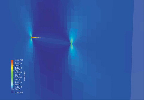
For RPV applications, Grizzly uses reduced-order models to efficiently compute SIFs for axis-aligned elliptical flaws, as described in Sec. III.A.2. Detailed XFEM models of cracks under the same conditions have been used to test the validity of those solutions, and initial testing has found them to be in very good agreement with each other. Using XFEM with interaction integrals also allows for straightforward evaluation of SIFs for flaws with more complex geometries, such as nonaxis-aligned flaws and multiple interacting flaws. Figure 2 shows a representative Grizzly simulation that uses XFEM and interaction integrals to compute SIFs for an embedded elliptical circumferential flaw in an RPV. The SIFs were directly computed from this detailed finite element model. A uniform 1-MPa far-field axial stress was imposed in this case. Although local mesh refinement was used in the vicinity of the flaw, the mesh does not conform to the flaw geometry, which is instead defined geometrically.

Fig. 2. Grizzly solution of an embedded elliptical circumferential flaw in an RPV showing cross section of the RPV wall passing through flaw with contours of von Mises stress (in Pa). Displacements are magnified 10 000$\times$ to show opening

III. RPV INTEGRITY ASSESSMENT

In LWRs the coolant and reactor internals are contained within the RPV, the integrity of which is critical for preventing the release of radioactive contaminants from the primary-coolant water during normal operation and transient conditions. RPVs are massive low-alloy ferritic steel vessels with a thin liner of stainless steel cladding on the inner surface. RPVs for pressurized water reactors (PWRs) are approximately 13 m tall, with an inner radius of approximately 2 m, while those for boiling water reactors are approximately 22 m tall, with an inner radius of approximately 3 m (Ref. 26).

Reactor pressure vessels contain potentially large populations of flaws introduced during the manufacturing process. Over their operating lives, RPVs are subjected to years of exposure to elevated temperature and pressure, including cyclic loading due to normal operations (startup, cooldown, testing, etc.), while also being subjected to neutron flux from the reactor. They are designed to withstand these normal operating conditions and must be demonstrated to have an acceptably low risk of failure during very rare beyond-design-basis accident conditions that could result in pressurized thermal shock (PTS) loading.^26,27 A PTS occurs when the RPV is flooded with lower-temperature coolant, resulting in a rapid decrease in the inner surface temperature while also being pressurized. The safety concern is that under one of these rare PTS events, a pre-existing flaw could serve as the initiation site for a fracture that could propagate through the wall. The steel is more brittle at lower temperatures, so the combined effects of low temperatures, high stresses (from thermal gradients and pressure loading), and embrittlement due to long-term exposure to the reactor environment increase the risk of fracture.

III.A. Analysis Procedure

Assessing the susceptibility of an embrittled RPV to fracture during a PTS event involves multiple distinct analysis phases: (1) computing the global thermomechanical response of the RPV to the transient loading, (2) performing a probabilistic fracture mechanics (PFM) analysis in which the probability of fracture initiation in any of the flaws present in the RPV is assessed, and (3) post processing the probabilistic results by combining them with the likelihood of occurrence of the transients studied.

Multiple codes are currently being developed for PFM analysis, as surveyed by Ref. 28, with PASCAL (Ref. 29) and FAVOR (Ref. 30) being the most widely used. Current codes used for this purpose are typically based on the assumption that there is no axial or azimuthal variation in the thermomechanical response of the RPV and treat the beltline region as an infinite cylinder, which permits solution of the global response with a one-dimensional (1-D) model. Grizzly follows the basic PFM approach used by the FAVOR code,³⁰ but adapts those algorithms to allow their use in more general conditions. For example, Grizzly allows for PFM calculations based on multidimensional models of the global thermomechanical RPV response and allows for the use of a 3-D fluence distribution to be read directly from data provided by a neutron-transport code.³¹

III.A.1. Global Thermomechanical Response

The process used for the analysis of the thermomechanical response of the RPV is a fairly standard application of coupling of the thermal and mechanical analysis features in the MOOSE modules. A finite element model of an RPV was constructed to include the relevant geometric features, including both the cladding and the base metal. Boundary conditions are prescribed to apply transient coolant temperature histories using convective flux boundary condition and pressure histories. Temperature-dependent thermal expansion and elastic moduli for the base and cladding materials are used in computing the material response.

Reactor pressure vessel integrity analyses typically focus on the behavior of the beltline region of the RPV that is in close proximity to the reactor core because that is the region that experiences the highest neutron fluence, and hence, the highest embrittlement. It is generally assumed that this region is sufficiently isolated from the ends of the vessel and the inlets to permit the idealization of its thermomechanical response as that of an infinite cylinder, which allows the use of a 1-D axisymmetric model for the global response. Grizzly allows for the use of 1-D global models, which require very little computational effort, but also allows for this global response to be modeled using two-dimensional (2-D) or 3-D representations, which allows for the investigation of the effects of spatial variations in the geometry and loading conditions.

Post processing is performed during each step of that analysis to perform least-squares fitting to compute the coefficients of polynomials that represent the through-wall variation of the temperature, hoop stress, and axial stress. These are used in the PFM analysis. For 1-D models, these coefficients are computed at a single location that represents the response everywhere in the RPV. For 2-D or 3-D models, the through-wall variations of these fields are computed at points on a regular grid in the azimuthal and axial coordinates in a cylindrical coordinate system and output for each of those grid point locations.

III.A.2. Probabilistic Fracture Mechanics

Due to the inherent uncertainty in the flaw population and the material properties of the RPV, probabilistic techniques are well suited to characterize the susceptibility of an RPV to fracture. The details of the PFM approach, as well as its implementation in Grizzly are described in detail in Ref. 32, and are only briefly summarized here.

In a PFM analysis, a series of random realizations of the population of flaws is generated using Monte Carlo sampling based on specified distributions of flaws in the RPV. Each flaw in the population is characterized by its geometric dimensions (size, position, orientation, aspect ratio), as well as parameters defining the local chemistry (concentrations of Cu, Ni, Mn, and P) and the nil-ductility reference temperature $R{T}_{NDT}$. A given realization of the flaw population often results in thousands of flaws in an RPV (based on experimental characterizations of flaw densities³³), the vast majority of which are usually found to be inconsequential in the PFM analysis.

Once the flaw population is generated, the local embrittlement of the material at that flaw location is computed. The semi-empirical model of Ref. 10 is currently used for this purpose, and including other models in a similar manner would be straightforward. This embrittlement is expressed as a shift in $R{T}_{NDT}$ from the value for the unirradiated material.

Because of the large number of flaws evaluated, it would be impractical to perform direct fracture mechanics simulations of each flaw. Instead a weight function approach originally proposed by Ref. 34 is used that computes $K_I$ as a linear superposition of contributions from individual components of a polynomial expansion of the far-field stress in the material where a crack is located.

In this technique, the through-wall distribution of the stress component normal to the crack $\sigma$ as a function of the depth $a{ }^{\mathrm{\prime }}$ relative to the flaw depth $a$ is described by an n’th-order polynomial:

(6) $\sigma \left(\frac{a{ }^{\mathrm{\prime }}}{a}\right)=C_0+C_1\left(\frac{a{ }^{\mathrm{\prime }}}{a}\right)+\cdots +C_n{\left(\frac{a{ }^{\mathrm{\prime }}}{a}\right)}^n,$(6)

where ${\mathit{C}}_i$ are the polynomial coefficients of the stress distribution. $K_I$ is computed as

(7) $K_I=\sum _{i=0}^n{C}_i{K}_i\sqrt{\pi a},$(7)

where $K_i$ are stress intensity factor influence coefficients (SIFICs). A given SIFIC $K_i$ is computed for a specific flaw geometry by evaluating $K_I$ using a finite element model or other approach that explicitly represents the flaw subjected to the far-field stress expansion of Eq. (6)(6) $\sigma \left(\frac{a{ }^{\mathrm{\prime }}}{a}\right)=C_0+C_1\left(\frac{a{ }^{\mathrm{\prime }}}{a}\right)+\cdots +C_n{\left(\frac{a{ }^{\mathrm{\prime }}}{a}\right)}^n,$(6) with all polynomial coefficients set to 0 except for $C_i$.

These SIFICs can be evaluated for a set of specific flaw geometries, and various techniques can be used to develop expressions for them over a range of parameters. This approach is adopted by the American Society of Mechanical Engineers (ASME) Boiler and Pressure Vessel Code, which provides formulas for computing SIFICs for surface-breaking and subsurface (embedded) elliptical flaws in Sec. XI, Article A-3000 of the ASME Boiler and Pressure Vessel Code.³⁵ There are some additional complexities for handling the effects of the cladding for surface-breaking flaws, as described in Ref. 32. It should also be noted that the approach for embedded flaws used in the present work is based on the technique of Ref. 36 to compute coefficients used in 2013 and earlier versions of the ASME code.

As mentioned in Sec. III.A.1, the stress coefficients at points on a grid in the azimuthal and axial coordinates are computed and output during the global RPV thermomechanical analysis. Every flaw evaluated in the PFM analysis falls at some point within this grid, and the polynomial coefficients describing the through-wall variation of a field at that point are interpolated from those grid points to the current point. The interpolated values of the stress coefficients are used in the $K_I$ calculation, and the interpolated values of the temperature coefficients are used to directly evaluate the temperature at the tip of the flaw being considered. Grizzly also provides the option of directly reading these stress and temperature fields from a mesh file. In that approach, stress is sampled at a set of points along a line emanating radially through the RPV wall, and least-squares fitting is performed to compute the stress coefficients. This approach was used in earlier work, but using precomputed polynomial coefficients in the PFM analysis has proven to be far more efficient.

Once $K_I$ is computed using the approach described previously, a Weibull statistical model is used to compute the conditional probability of fracture initiation (CPI) of each flaw, given occurrence of the transient, at each time. This model uses a closed-form expression that is as a function of $K_I$, the current temperature at the flaw location, and $R{T}_{NDT}$ with the effect of embrittlement. This is used to compute the aggregate CPI for any flaw in the RPV $\mathrm{C}\mathrm{P}{\mathrm{I}}_{\mathrm{R}\mathrm{P}\mathrm{V}}$ as

(8) $\mathrm{C}\mathrm{P}{\mathrm{I}}_{\mathrm{R}\mathrm{P}\mathrm{V}}=1-\prod _{i=1}^{n_{\mathrm{f}\mathrm{l}\mathrm{a}\mathrm{w}}}(1-\mathrm{C}\mathrm{P}{\mathrm{I}}_i),$(8)

where $n_{\mathrm{f}\mathrm{l}\mathrm{a}\mathrm{w}}$ is the number of flaws in the RPV, and $\mathrm{C}\mathrm{P}{\mathrm{I}}_i$ is the maximum CPI for flaw $i$ during that transient.

$\mathrm{C}\mathrm{P}{\mathrm{I}}_{\mathrm{R}\mathrm{P}\mathrm{V}}$ computed in Eq. (8)(8) $\mathrm{C}\mathrm{P}{\mathrm{I}}_{\mathrm{R}\mathrm{P}\mathrm{V}}=1-\prod _{i=1}^{n_{\mathrm{f}\mathrm{l}\mathrm{a}\mathrm{w}}}(1-\mathrm{C}\mathrm{P}{\mathrm{I}}_i),$(8) represents the CPI for a particular realization of the flaw population. Usually, a very small number of flaws in a given population have nonzero values of CPI, and there is typically significant variation in the value of $\mathrm{C}\mathrm{P}{\mathrm{I}}_{\mathrm{R}\mathrm{P}\mathrm{V}}$ from one RPV realization to the next. The primary quantity of interest in a PFM calculation is the mean value of $\mathrm{C}\mathrm{P}{\mathrm{I}}_{\mathrm{R}\mathrm{P}\mathrm{V}}$ computed over a set of RPV realizations that is sufficiently large that $\mathrm{C}\mathrm{P}{\mathrm{I}}_{\mathrm{R}\mathrm{P}\mathrm{V}}$ does not change significantly with the addition of more realizations. At that point, these Monte Carlo iterations are considered to be converged.

If $\mathrm{C}\mathrm{P}{\mathrm{I}}_{\mathrm{R}\mathrm{P}\mathrm{V}}$ is very low, which is often the case, a large number of RPV realizations is usually required for convergence. It is thus essential for computational efficiency for the evaluations of individual flaws to be very rapid, and parallel computation greatly aids in these calculations. In Grizzly, the PFM calculation is performed as a separate analysis after the global analysis. This calculation does not perform PDE solutions as is typically the case in a MOOSE-based application, but it takes advantage of many of the features of MOOSE to efficiently perform these calculations in parallel.

III.B. PFM Demonstration with Plume Effect

The current standard practice in RPV PFM calculations is to assume that temperature and pressure are applied uniformly to the RPV during a transient. This, in combination with an assumption that the beltline region of interest is sufficiently distant from geometric features that would affect its response under such conditions, allows the RPV’s global response to be computed using a 1-D axisymmetric model. The assumption of uniform coolant temperature can be called into question, however, because as the RPV is flooded with lower-temperature coolant, the temperature in the region near the inlet will be lower than that in the rest of the vessel until sufficient time has passed for mixing to occur.

Other researchers^37,38 have recently investigated this “cold plume” effect and shown that the more rapid cooling in the plume region near the inlet results in higher SIFs and fracture probabilities in this region. These studies focused on a limited number of specific flaws in selected regions of an RPV.

Because of its ability to perform PFM calculations based on multidimensional analyses of the global RPV response, Grizzly is uniquely able to evaluate the cold plume effect in a probabilistic analysis that considers the full flaw population in an RPV rather than investigating isolated flaws. This capability is demonstrated here using a 3-D quarter-symmetry model of a representative full RPV, including all relevant geometric effects, with a postulated transient with a nonuniform temperature distribution.

III.B.1. Global Thermomechanical Analysis

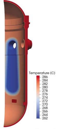
The RPV geometry and dimensions used here are based on publicly available information on a typical four-loop PWR pressure vessel, but do not represent a specific RPV. To idealize the nonuniform temperature conditions, a plume region emanating downward from the inlet is identified, as shown on the model in Fig. 3. A transient temperature and pressure history that has been used in other PTS analyses assuming spatially uniform conditions is used as the basis for the transient applied here and is applied to the balance of the inner surface of the RPV, while a more rapidly decreasing temperature function is used in the plume region. As can be seen in Fig. 3, which shows the temperature at time = 120 s there is a region between the plume and nonplume regions over which the temperature linearly transitions between the two functions.

Fig. 3. Quarter-symmetry 3-D RPV model used in plume effect demonstration. Temperature contours shown at 120 s into the simulation during the rapid cooling phase to identify the region where the cold plume was applied (shown in blue)

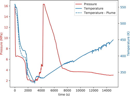
The transient that is used as the basis for this nonuniform temperature distribution is particularly aggressive and represents a scenario in which a pressure release valve is stuck open, resulting in depressurization and significant decrease in temperature followed by a rapid repressurization and slow temperature increase once the valve closes again. Figure 4 shows the pressure and temperature histories applied in both the plume and nonplume regions. The plume temperature history was created as an offset to the nonplume baseline function such that the maximum temperature difference between the plume and nonplume region is 20°C. The plume function drops the temperature more quickly than the nonplume region for the first 3000 s until it reaches the same temperature as the rest of the inner surface, and then the functions are the same.

Fig. 4. Internal pressure and temperature loading histories used for RPV PFM analysis. Temperature histories applied to the plume and nonplume region are both shown, and the single pressure history shown is applied to the entire RPV inner surface

It is important to emphasize that this is a contrived example created to demonstrate this capability in Grizzly. The shape and size of the plume region, as well as the temperature difference between the plume and nonplume region, are approximations and do not represent actual expected conditions. High-fidelity computational fluid dynamics (CFD) simulations could be used to compute more realistic transient coolant-temperature distributions.

The RPV model used in this study has the dimensions and other constant properties listed in Table I. Temperature-dependent material properties for the base metal and stainless steel liner were used for the base metal and cladding materials, respectively. Tabular functions were used for these temperature-dependent properties, and Table II provides samples of these properties at three temperatures relevant for this simulation. It should be noted that the thermal expansion coefficients are mean values, with the reference temperature shown in Table I. Appropriate symmetry conditions were applied to the model shown in Fig. 3 to allow it to represent the response of the full RPV, assuming that all inlets experience the same plume effects.

TABLE I Constant Values Used in Global RPV Simulation

RPV total wall thickness	219.2 mm
Cladding thickness	4.064 mm
RPV inner radius	2.197 m
Thermal expansion reference temperature	21.1°C
Stress free temperature	253.3°C
Convective flux heat transfer coefficient	5.0 kW/(m${ }^2$K)
Base and cladding Poisson’s ratio	0.3
Base and cladding density	7833 kg/m${ }^3$
Operating temperature	286.1°C

TABLE II Temperature-Dependent Material Properties for the Base Metal and Cladding Used in the Global RPV Simulation at Selected Temperatures

Property	Value at 286°C	Value at 177°C	Value at 67°C
Base Young’s Modulus (GPa)	184.2	191.0	198.3
Clad Young’s Modulus (GPa)	127.0	135.8	147.3
Base coefficient of thermal expansion (K${ }^{-1}$)	1.395 $\times {10}^{-5}$	1.350 $\times {10}^{-5}$	1.291 $\times {10}^{-5}$
Clad coefficient of thermal expansion (K${ }^{-1}$)	1.701 $\times {10}^{-5}$	1.638 $\times {10}^{-5}$	1.562 $\times {10}^{-5}$
Base thermal conductivity (W/m$\cdot$K)	41.52	43.25	43.42
Clad thermal conductivity (W/m$\cdot$K)	18.34	16.61	14.88
Base specific heat (J/Kg$\cdot$K)	555.2	512.1	461.0
Clad specific heat (J/Kg$\cdot$K)	546.8	526.7	500.7

To quantify the effect of the plume, two versions of the model were run: one with separate temperature histories applied to the plume and nonplume regions, and a baseline case in which the nonplume baseline temperature history is applied everywhere in the inner surface of the RPV. The heat transfer coefficient in general varies spatially and temporally over the course of the transient, but because a full CFD analysis would be required to establish this for a spatially varying temperature, a constant value of 5000 W/(m${ }^2$K) was used throughout the analysis.

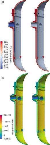
Figure 5 shows representative temperature and hoop-stress contours computed using this 3-D model for the cases with and without the plume effect at a time when the differences between the two are most pronounced. The same color scales are used for both cases, and it can be clearly seen that the material in the plume region experiences both lower temperatures and higher tensile hoop stresses due to the more rapid cooling. The model is clipped through the centerline of the inlet to show the through-wall variations of these fields and their spatial variation at the location where the differences are most pronounced.

Fig. 5. (a) Temperature and (b) hoop-stress contours in the 3-D global RPV model 420 s into the transient event. Results for the case with and without the plume are shown on the left and right, respectively

III.B.2. PFM Analysis

Two separate PFM analyses were performed based on the plume and nonplume global RPV analyses described previously. The PFM analysis depends on user-defined flaw distributions, parameters describing material chemistry and toughness, the fluence distribution, and the locations of welds. The parameters used for the PFM analysis were intentionally kept simple to highlight the effects of the plume in this analysis.

Reactor pressure vessels are manufactured by welding together plates or forgings, and these weld regions typically have properties that make them more susceptible to fracture than the plates or forgings. Although these welds can be represented in Grizzly, the model used for this demonstration consists of a single cylindrical plate spanning a 90-deg quadrant of the vessel. Because welds tend to have higher densities of flaws with higher probabilities of failure, including them would make it more challenging to see the effects of the plume. Likewise, the fluence distribution can be quite complex, and full 3-D maps of the fluence distribution can be read in from a file in Grizzly, but instead, a constant surface fluence was prescribed, and the equation of Ref. 39 was used to attenuate the fluence through the wall.

To define the flaw density, depth, and aspect ratios, a set of distributions based on data in Ref. 33 was used, and only embedded flaws were considered. The plate was assumed to have been exposed to 40 effective full power years, with an inner surface fluence of $0.327\times {10}^{19}/\mathrm{c}{\mathrm{m}}^2$. Coefficients of variation of 0.118 and 0.056 were used for sampling the fluence for the full plate and for individual flaws within that plate. The mean values of the concentration of alloying elements (in weight percent) in the plate were Cu = 0.13, Ni = 0.7, Mn = 1.44, and P = 0.01. Standard deviations of the normal distributions for Cu, Ni, and P were 0.0073, 0.0244, and 0.0013, respectively. Sampling the Mn concentration uses a more complex process with no user-settable parameters. The unirradiated nil-ductility reference temperature $R{T}_{NDT0}$ is 10.0°C, and its standard deviation is 9.44°C.

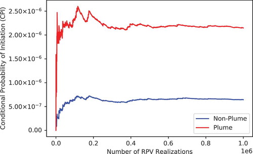
Figure 6 shows the convergence history of the Monte Carlo iterations for the plume and nonplume cases and how a large (1 $\times {10}^6$) number of RPV realizations would need to be evaluated before these results could be considered converged. The plume case clearly shows an increased likelihood of failure, with a mean CPI for the quarter of the RPV considered of 2.15 $\times {10}^{-6}$, as opposed to a value of 6.44 $\times {10}^{-7}$ for the nonplume case.

Fig. 6. Convergence history of Monte Carlo iterations for computing CPI for plume and nonplume PFM models

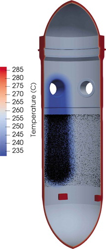
Figure 7 shows the distribution of flaws with nonzero failure probability from the 1 $\times {10}^6$ Monte Carlo iterations superimposed on a snapshot of the temperature distribution during the transient for the plume case. It is important to note that these are not flaws in an individual RPV realization, but the accumulation of flaws over a large number of realizations. This clearly illustrates how there is an increased propensity for flaw failure in the plume region, which is due to a combination of the higher thermally induced stresses and lower temperatures in that region.

Fig. 7. Locations of flaws with nonzero CPI over 1 $\times {10}^6$ Monte Carlo iterations superimposed on the RPV global model, showing the temperature field at a point during the cooldown phase of the transient

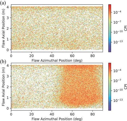
Figure 8 shows scatter plots of the flaws for the plume and nonplume cases, but in a 2-D rollout plot with the flaw positions color coded by CPI and plotted in terms of axial versus azimuthal coordinates, with the origin being a point at the lower right side of the beltline region in Fig. 7. These plots clearly show how in the plume case there is a significantly higher density of flaws with high CPI in the plume region, while the flaws with nonzero CPI are much more uniformly distributed in the nonplume case.

Fig. 8. Locations of all flaws with nonzero CPI over 1 $\times {10}^6$ Monte Carlo iterations in terms of azimuthal and axial position in the RPV. Results are shown for the (a) uniform temperature (nonplume) PFM model and (b) plume model. Flaws are colored based on CPI, and the origin of this coordinate system is at the lower right side of the beltline region in the model shown in Fig. 7

As mentioned previously, the scenarios considered here were simplified considerably in several ways to highlight the effect of the plume, and as a result, these analyses clearly show this. Future studies will include more realism in all aspects of the model, including adding the effects of welds, nonuniform fluence maps, and more realistic thermal boundary conditions. The effects of the plume will likely not be as pronounced in such models as they are here because of the other sources of spatial nonuniformity.

IV. CONCRETE DEGRADATION MODELING

Concrete is widely used in the construction of nuclear facilities due its structural strength and ability to shield radiation. Notable uses of concrete in LWR nuclear power plant structures include biological shield walls, containment structures, spent fuel pools, and cooling towers. Concrete usually has a long life span; however, when exposed to extreme environments such as high temperatures, humidity, chemical attack, etc., the performance of the concrete can degrade significantly. Hence, understanding the aging and degradation of concrete over time is essential to ensure the performance, operability, and safety of nuclear facilities.

Concrete degradation is a complex phenomenon that can involve multiple physical and chemical mechanisms. For example, long-term degradation of concrete in nuclear power plant structures is influenced by its exposure to temperature, humidity, radiation, loading, chemical seepage, etc. The properties of the constituents of the concrete, such as aggregates, cement, and reinforcement bars also significantly influence the mechanical behavior and strength of the concrete.

Coupling between the physical phenomena involved in concrete degradation is often important. For example, multiple mechanisms that affect mechanical behavior depend on local temperature and moisture, which can have significant spatial and temporal variation depending on the boundary conditions. Likewise, mechanical damage can affect moisture and chemical transport. Hence, modeling long-term concrete degradation requires having the ability to model each of the physics individually as well as coupled together. A variety of approaches have been taken to address coupling between the physics models relevant to concrete degradation, including one-directional coupling and multidirectional coupling,^40–45 depending on the needs of specific applications.

Some concrete structures in nuclear power plants are exposed to significantly more aggressive environments than typically experienced by usual civil engineering structures. Degradation mechanisms that have been identified as being particularly significant for the nuclear industry include expansion due to alkali-silica reaction⁴⁶ (ASR) and radiation-induced volumetric expansion⁴⁷ (RIVE), which both lead to strength reduction, damage, and microcracking in the concrete. While ASR is observed in a variety of civil structures, RIVE is unique to nuclear applications.

The ASR deterioration of concrete structures can be attributed, on the microscopic level, to the formation of a hydrophilic gel due to complex dissolution-precipitation reactions between reactive silica in aggregates and alkaline ions such as potassium (K${ }^{+}$), sodium (Na${ }^{+}$), and hydroxyl (OH${ }^{-}$) in the cement-pore solution. If water is available in concrete pores, the gel swells, creating internal pressure in localized regions within concrete structures that can initiate micro and macro cracking, excessive expansion, misalignment of structures, etc. In addition, exposure to higher temperatures and humidity can significantly accelerate the ASR reaction rate. The prediction of ASR thus requires a fully coupled thermohydromechanical model that captures the spatial and temporal evolution of temperature, humidity, stress, and strain, including the long-term creep and stress relaxation in the concrete.

IV.A. Model Details

Grizzly and BlackBear have a maturing capability for modeling the moisture and thermal transport processes in concrete that contribute to the progression of multiple degradation mechanisms. They can also model expansive reactions and their effects on mechanical response and strength. The thermal, moisture, and mechanical models are all solved in a tightly coupled manner that permits capturing multidirectional coupling between these models. BlackBear provides the foundational set of physics models for concrete, including models for the nonlinear mechanical response of concrete and reinforcing bars, all available as open-source software.¹⁸ Details of a basic set of models used for modeling ASR are described here. Grizzly also provides a model for RIVE, not described here, which employs some of the foundational models provided by BlackBear.

The ability to solve coupled multiphysics equations provides an essential foundation for a concrete degradation modeling tool. Grizzly and BlackBear leverage the features of the MOOSE framework that greatly facilitate the solution of the coupled physics equations relevant to concrete. This solution environment makes it natural to solve coupled equations such as these in a single, tightly coupled nonlinear solution algorithm. Adding dependencies of any of these physics models on the variables associated with other physics is also made quite straightforward by the modular nature of MOOSE and the facilities provided for coupling. For example, it has been demonstrated that the foundational models discussed here can be readily built upon to include complex coupling between chemical species transport models as well as reactions between those species.^48,49

IV.A.1. Heat Transfer

The governing PDE for heat transfer in concrete is an extension of the heat equation given by Bazant et al.⁵⁰ and Saouma et al.⁵¹ as

(9) $\rho C\frac{\mathrm{\partial }T}{\mathrm{\partial }t}=\mathrm{\nabla }\cdot \left(k\mathrm{\nabla }T\right)-C_w{D}_h\mathrm{\nabla }H\mathrm{\nabla }T+C_a\frac{\mathrm{\partial }W}{\mathrm{\partial }H}\frac{\mathrm{\partial }H}{\mathrm{\partial }t}+Q,$(9)

where

$T$ =	=	temperature
$\rho$ =	=	density of the concrete
$C$ =	=	specific heat
$k$ =	=	thermal conductivity of the concrete
$C_w$ =	=	mass density and isobaric (constant pressure) heat capacity of liquid water
$W$ =	=	water (moisture) content
$H$ =	=	pore water relative humidity
$C_a$ =	=	heat absorption of free water
$\frac{\mathrm{\partial }W}{\mathrm{\partial }H}$ =	=	moisture capacity
$Q$ =	=	rate of heat per unit volume generated within the body
$t$ =	=	time.

The terms on the right side of Eq. (9)(9) $\rho C\frac{\mathrm{\partial }T}{\mathrm{\partial }t}=\mathrm{\nabla }\cdot \left(k\mathrm{\nabla }T\right)-C_w{D}_h\mathrm{\nabla }H\mathrm{\nabla }T+C_a\frac{\mathrm{\partial }W}{\mathrm{\partial }H}\frac{\mathrm{\partial }H}{\mathrm{\partial }t}+Q,$(9) represent heat conduction, convective transport of heat due to fluid flow, and heat adsorption due to the adsorption of free water molecules in pores onto pore walls, respectively.

There are several constitutive models available in BlackBear to calculate the thermal capacity $\rho C$ and thermal conductivity $k$ of the concrete such as the American Society Civil Engineering model⁵² for normal-strength concrete, the Kodur model⁵³ for high-strength concrete, and the Eurocode model⁵⁴ for both normal- and high-strength concrete. Details of these models can be found in Ref. 48.

IV.A.2. Moisture Diffusion

The governing equation for moisture diffusion in concrete is formulated based on solving for the pore water relative humidity $H$ as a field variable:

(10) $\frac{\mathrm{\partial }W}{\mathrm{\partial }H}\frac{\mathrm{\partial }H}{\mathrm{\partial }t}=\mathrm{\nabla }(D_h\mathrm{\nabla }H)+\mathrm{\nabla }(D_{ht}\mathrm{\nabla }T)+\frac{\mathrm{\partial }{W}_d}{\mathrm{\partial }t},$(10)

where

$W$ =	=	total water content
$D_h$ =	=	moisture diffusivity
$D_{ht}$ =	=	coupled moisture diffusivity under the influence of a temperature gradient
$W_d$ =	=	a source term representing the total mass of free evaporable water released into the pores by dehydration of the cement paste.

Similar to thermal properties, there are several models available in BlackBear for calculating the properties associated with relative humidity evolution.⁴⁸

IV.A.3. ASR Swelling

Based on Ulm et al.’s stress-independent reaction,⁴⁰ Saouma and Perotti proposed a first-order ASR reaction kinetics model that is dependent on both the temperature and the first invariant of the stress tensor⁵⁵ as

$t_C(\theta ,\xi )\cdot \frac{d\xi }{dt}={\tau }_C(\theta )\cdot \frac{1+\mathrm{e}\mathrm{x}\mathrm{p}[-{\tau }_L(\theta ,I_{\sigma },f_{c{ }^{\mathrm{\prime }}})/{\tau }_C(\theta )]}{\xi +\mathrm{e}\mathrm{x}\mathrm{p}[-{\tau }_L(\theta ,I_{\sigma },f_{c{ }^{\mathrm{\prime }}})/{\tau }_C(\theta )]}\cdot \frac{d\xi }{dt}=1-\xi ,$

where

$\xi$ = ASR reaction extent, ranging from 0 (not reacted) to 1 (fully reacted)

$\theta$ = temperature (the symbol $\theta$ is used instead of $T$ for temperature to be consistent with the notations in Refs. 40 and 55)

${\tau }_C(\theta )$, ${\tau }_L(\theta ,I_{\sigma },f_{c{ }^{\mathrm{\prime }}})$ = the latency and characteristic times of ASR reactions expressed as

(11) ${\tau }_C(\theta )={\tau }_C({\theta }_0)\mathrm{e}\mathrm{x}\mathrm{p}[U_C(1/\theta -1/{\theta }_0)]$(11)

and

(12) ${\tau }_L(\theta ,I_{\sigma },f_c\mathrm{\prime })=f(I_{\sigma },f_c\mathrm{\prime }){\tau }_L({\theta }_0)\mathrm{e}\mathrm{x}\mathrm{p}[U_L(1/\theta -1/{\theta }_0)],$(12)

respectively, where

${\theta }_0$ =	=	reference temperature for free ASR expansion
$I_{\sigma }$ =	=	first invariant of the stress tensor
$f_{c{ }^{\mathrm{\prime }}}$ =	=	uniaxial compressive strength of concrete
$U_L$, $U_C$ =	=	thermal activation energy constants for the latency and characteristic times, respectively.

The function $f(I_{\sigma },f_{c{ }^{\mathrm{\prime }}})$ represents the effect of compressive stress, which can impact the ASR reaction kinetics by delaying the latency time ${\tau }_L$ (Refs. 48 and 55). Equation (11)(11) ${\tau }_C(\theta )={\tau }_C({\theta }_0)\mathrm{e}\mathrm{x}\mathrm{p}[U_C(1/\theta -1/{\theta }_0)]$(11) for the ASR reaction is a nonlinear ODE that can be solved locally in an incremental form utilizing a Newton-Raphson iteration scheme, given the current temperature, the stress, and the reaction extent at the end of the previous time step.

From the ASR reaction extent $\mathrm{\Delta }\xi$, the ASR volumetric strain increment $\mathrm{\Delta }{\epsilon }_{vol}^{\mathrm{A}\mathrm{S}\mathrm{R}}$ from time $t$ to $t+\mathrm{\Delta }t$ is evaluated using

(13) $\mathrm{\Delta }{\epsilon }_{vol}^{\mathrm{A}\mathrm{S}\mathrm{R}}={\mathrm{\Gamma }}_t(f_{t{ }^{\mathrm{\prime }}},{\sigma }_1|COD){\mathrm{\Gamma }}_c(\bar{\sigma },f_{c{ }^{\mathrm{\prime }}})g(H)\mathrm{\Delta }\xi {\epsilon }^{\mathrm{\infty }}{|}_{\theta ={\theta }_0},$(13)

where

$f_{t{ }^{\mathrm{\prime }}}$ =	=	tensile strength of the concrete
${\sigma }_I$ =	=	maximum principal stress
$COD$ =	=	crack opening displacement
$\bar{\sigma }$ =	=	ratio between the hydrostatic stress and compressive strength of concrete
${\epsilon }^{\mathrm{\infty }}$ =	=	maximum free volumetric expansion at the reference temperature.

The function $g(H)$ describes the dependency of gel expansion on the water in concrete such that $g(H)=H^m$, with $m$ being an empirical constant known as relative humidity exponent. Functions ${\mathrm{\Gamma }}_c(\bar{\sigma },f_{c{ }^{\mathrm{\prime }}})$ and ${\mathrm{\Gamma }}_t(f_{t{ }^{\mathrm{\prime }}},{\sigma }_{\hspace{0.17em}}1|COD)$ account for the reduction in ASR expansion due to absorption of gel into diffuse microcracks in compressive loading or into tensile cracks, respectively.⁵⁵

The ASR expansion is anisotropic, and this is represented in the model by redistributing the incremental ASR volumetric strain $\mathrm{\Delta }{\epsilon }_{vol}^{\mathrm{A}\mathrm{S}\mathrm{R}}$ in the three principal directions according to their relative propensity for expansion. Saouma and Perotti⁵⁵ presented a method to calculate the relative weights along three principal directions based on the principal stresses under either uniaxial, biaxial, or triaxial confinement conditions. Details of the approach along with the implementation strategy are provided in Ref. 48. The individual incremental ASR strains in the principal directions are obtained using the relative weights $W_i$:

(14) $\begin{array}{cccc}\mathrm{\Delta }{\epsilon }_i^{\mathrm{A}\mathrm{S}\mathrm{R}}\mathit{=}{W}_i\Delta {\epsilon }_V^{\mathrm{A}\mathrm{S}\mathrm{R}}\mathit{,}& i=1,2,3.& \hspace{0.17em}& \hspace{0.17em}\end{array}$(14)

These strains differ from each other in general, depending on the local stress state driven by the material confinement conditions. This ASR expansion-induced strain is imposed as an incremental eigenstrain during the mechanical solution in BlackBear to calculate the overall deformation of the concrete structures.

IV.A.4. Concrete Creep

Creep deformation is observed in concrete under sustained loading over time. Creep is facilitated by external conditions, such as temperature, moisture, etc., that lead to the shrinkage of concrete over time. Here, the creep behavior of the concrete material is modeled based on the generalized Kelvin-Voigt model,⁵⁶ where the system is represented by a combination of springs and dashpots connected in a series. The viscoelastic behavior of the dashpots deteriorates the effective stiffness of the concrete. The overall stress-strain behavior is expressed as

(15) ${\sigma }_{ij}=C_{ijkl}{\epsilon }_{kl}^{mech}-\sum _{n=1}^N{C}_{ijkl}^n{\alpha }_{kl}^n,$(15)

where ${\alpha }^n$ are internal strains associated with each Kelvin-Voigt unit, and ${\mathit{C}}^n$ is the stiffness of the corresponding spring in the chain. These units obey the following time-dependent relationship:

(16) $\mathrm{\forall }n\in [1,N]:{\sigma }_{ij}^n=C_{ijkl}^n\left({\alpha }^n+{\eta }^n{\dot{\alpha }}^n\right),$(16)

where ${\eta }^n$ is the viscosity of the associated dashpot. The constitutive equations are solved using a semi-implicit, single-step, first-order finite difference scheme.

Further, the logarithmic viscoelastic behavior for concrete has been implemented assuming a Burgers-type of material with an elastic spring, a Kelvin-Voigt module, and a dashpot placed in series. The total strain is decomposed into three components: an elastic strain ${\epsilon }_{\mathbf{e}}$, a recoverable viscoelastic strain ${\epsilon }_{\mathbf{r}}$, and an irrecoverable creep strain ${\epsilon }_{\mathbf{c}}$, such that

(17) $\mathit{\epsilon }={\epsilon }_e+{\epsilon }_r+{\epsilon }_c.$(17)

Elastic strain is directly related to the stress $\mathbf{s}$ with the usual Hooke’s law. Recoverable creep strain corresponds to the short-term viscoelastic strain of the material, which can be partially recovered upon unloading. It is calculated using a single Kelvin-Voigt module:

(18) $\sigma ={\mathit{C}}_r:\left({\mathit{\epsilon }}_r+{\eta }_r{\dot{\mathit{\epsilon }}}_r\right),$(18)

where ${\mathit{C}}_r$ is the fourth-order elasticity tensor of the spring, and ${\eta }_r$ is the viscosity of the dashpot. Irrecoverable creep strain corresponds to the long-term viscoelastic strain of the material. It is linear with the logarithm of time, and is calculated as

(19) $\sigma =\left(1+\frac{t}{{\tau }_c}\right){\eta }_c{C}_e:\stackrel{.}{{\epsilon }_c},$(19)

where ${\eta }_c$ is the viscosity of the time-dependent dashpot, and ${\tau }_c$ is the characteristic time of the logarithmic creep that controls when the logarithmic behavior starts. The model also includes the effect of temperature, relative humidity, and drying on creep.

IV.A.5. Damage Model

Alkali-silica reaction expansion causes microcracking in the ASR-affected regions, resulting in the degradation of the local mechanical properties of the concrete. These effects are represented using the following scalar damage model⁵⁵ in BlackBear:

(20) $d=(1-{\beta }_E)\xi ,$(20)

where

$d$ =	=	damage index induced by ASR
$\xi$ =	=	ASR extent
${\beta }_E$ =	=	residual fraction of elastic modulus at full ASR reaction.

The damage reduces the effective elastic modulus, which affects the stress calculation

(21) $\sigma =(1-d)\mathit{C}:{\mathit{\epsilon }}_e,$(21)

where

$\sigma$ =	=	damaged stress
$\mathit{C}$ =	=	undamaged elasticity tensor
${\mathit{\epsilon }}_e$ =	=	elastic strain computed by subtracting the inelastic contributions from the total strain.

It should be noted that this isotropic damage model does not fully capture the effects of external loading on the orientation of ASR-induced microcracks.⁵⁷

The effects of damage can be accounted for in conjunction with creep and plasticity in BlackBear. First, the inelastic strains accounting for various deformation mechanisms, such as plasticity, creep, etc., and the corresponding effective stresses are calculated based on the undamaged properties using an iterative process. The damage index is then applied to the effective stress to calculate the damaged stress. Although only ASR-induced damage is discussed here, BlackBear also has the ability to include other sources of damage, such as those induced by mechanical loading.

IV.A.6. Reinforcing Bars

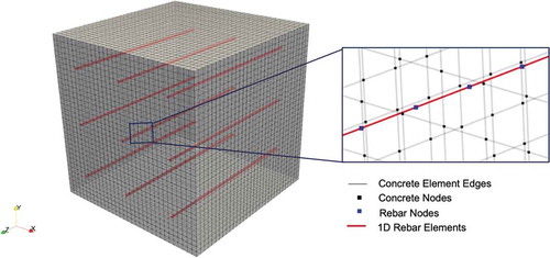
Most concrete structures contain reinforcing bars (rebar) to improve their ability to carry tensile stresses. For structural-scale simulations, it is generally impractical to explicitly include rebar in the mesh in higher-dimensional models. BlackBear provides an ability to represent rebar using discrete 1-D truss elements in models where the concrete is represented using 2-D or 3-D continuum elements.

Creating higher-dimensional meshes of the concrete that conform to the rebar is inherently problematic. To simplify the process of mesh creation, BlackBear uses node-to-element constraints to connect the nodes of the rebar to the continuum elements in which they are located. These constraints are very general and can be used to enforce that the value of any solution variable at a node is equal to the interpolated value of a solution variable at its location in a 2-D or 3-D continuum element.

The primary advantage of this approach is that it does not require coincident nodes or conforming meshes between concrete and rebar. This allows the mesh of the concrete structure to be completely independent of the mesh of the 1-D rebar elements. For every node in the rebar mesh, the containing concrete element is identified, and a constraint is imposed between the rebar node and the set of nodes in the concrete element.

The equal-value constraint acts upon overlapping portions of two blocks using a penalty-based formulation. The error in the solution is proportional to a user-specified penalty parameter $k_p$, which is set to a value sufficiently high to minimize error. The constraint is enforced by updating the residual on the secondary (rebar) nodes $r_s$ and primary (concrete) nodes $r_p$ as

(22) $\begin{array}{cc}{r}_s& =r_s+k_p(u_s-u_p)\\ \mathrm{a}\mathrm{n}\mathrm{d}\\ r_p& =r_p-\sum _{i=0}^n{\varphi }_i{k}_p(u_s-u_p),\end{array}$(22)

where

$u_s$ =	=	value of the solution field on the secondary nodes
$u_p$ =	=	corresponding value of that field interpolated from its values at the primary nodes at its location in the concrete element
${\varphi }_i$ =	=	interpolation function associated with node $i$ in the primary element
$n$ =	=	number of nodes in the primary element.

This formulation assumes no bond slip between the concrete and rebar, but this effect can be included in the constraint.

In the present study, the constitutive behavior of the rebar is assumed to be linearly elastic, with a constant coefficient of thermal expansion, but more complex behavior can be readily included.

IV.B. ASR Model Demonstration

Development of a set of tests to validate the concrete models in BlackBear against experimental data is currently underway, and one of these test cases is shown here to demonstrate these modeling capabilities. Wald et al.⁵⁸ performed a series of experiments to understand how the presence of multiaxial reinforcement affects the ASR expansion behavior of concrete. In their study, multi-axial expansion was monitored for a set of 33 reinforced concrete cubes, all having the same size (480 mm), but with varying reinforcement configurations. These cubes were exposed to temperature and humidity conditions designed to result in accelerated ASR. Four unreinforced specimens were monitored to obtain the free expansion behavior of the concrete. These experiments are well suited to assess the ability of the rebar models in BlackBear to predict the confining effect of rebar on concrete structures affected by ASR.

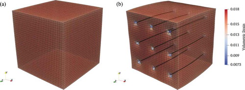
Two of these experiments are modeled here: one unreinforced block (Specimen A1-000b) and one block with nine uniaxial bars oriented in the z-direction (Specimen A1-001a). Figure 9 shows the BlackBear model of the block with rebar modeled as 1-D trusses. This shows the configuration of the nine bars oriented in the z-direction, distributed in three uniform layers. The concrete is modeled with a uniform $32\times 32\times 32$ mesh of linear hexahedral elements, while each rebar is meshed with 23 elements along its axial dimension. As can be seen from the close-up view provided in Fig. 9, the nodes of the rebar mesh do not necessarily coincide with the nodes of the concrete mesh. The model of the unreinforced block is not shown, but is identical except for the absence of rebar. The constraints described in Sec. IV.A.6 were used to tie the nodes of the rebar to the concrete elements.

Fig. 9. BlackBear model of concrete block for a case with nine reinforcing bars aligned with the z-direction (Specimen A1-001a). The close-up view shows details of the independent meshing of the rebar and concrete continuum

Because of the relatively small size of this experimental specimen, there is not significant spatial variation in the temperature and relative humidity fields. Nonetheless, the BlackBear models of these blocks solved for temperature, relative humidity, and displacement fields using the models described in this paper. Other applications more suitable for highlighting the effects of coupling have been demonstrated on more hypothetical scenarios.⁵⁹ The mechanical model included ASR expansion and creep in the concrete. Table III shows the material properties used in the BlackBear models. The only mechanical boundary conditions applied to the blocks were pinned constraints to prevent rigid body motion but allow unrestrained free expansion. For thermal and humidity boundary conditions, experimental temperature and humidity histories,⁵⁸ as shown in Fig. 10, are applied on all outside boundaries of the concrete blocks.

TABLE III Properties of the Concrete

Material Property	Value
Initial temperature	10.6°C
Initial relative humidity	80%
Aggregate type	Siliceous
Reference density	2231 kg/m^3
Reference specific heat	1100.0 J/(kg K)
Water/cement ratio	0.5
Aggregate volume fraction	0.7
Concrete Young’s Modulus	37.9 GPa
Rebar Young’s Modulus	200 GPa
Concrete Poisson’s ratio	0.22
Rebar thermal expansion coefficient	$11.3\times {10}^{-6}$/K
Rebar thermal conductivity	53 W/(m K)
ASR expansion characteristic time	18.9 days
ASR expansion latency time	18 days
ASR characteristic. activation Energy	5400
ASR latency activation energy	9400
ASR reference temperature	35°C
Activation temperature for creep	23°C

Fig. 10. (a) Time history of temperature and (b) relative humidity, including reported values from experiments⁵⁸ applied to the boundary of the BlackBear model along with average values computed in the plain and reinforced blocks in the BlackBear models

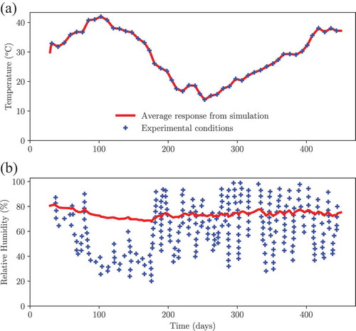
In the simulations, the average temperature response of the block closely follows the environmental temperature prescribed on the boundaries of the block because heat conduction occurs rapidly relative to the timescale of the experiment. However, due to the low permeability of the concrete, moisture transport occurs over much longer timescales, and the average value of the relative humidity can differ significantly from the value at the boundary, as shown in Fig. 10, which compares the computed average temperature and relative humidity in the concrete block with the values applied at the boundaries.

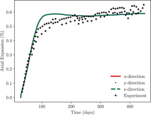
During the experiments, the axial expansion in three directions was monitored. These measurements include all sources of expansion, which include ASR and thermal expansion. Since data for ASR expansion in isolation are not available, the parameters that control the ASR expansion model were calibrated to match the average axial expansion reported in the plain concrete block. The displacement values were extracted from the simulation at the same six points that were considered during the experiments⁵⁸ on each of the surfaces. The average expansion, here, represents the average of measurements from these six points. Considering the curing time of 28 days, the simulations were started at 28 days except otherwise mentioned. Figure 11 shows the experimental and simulation results, which indicate that, with calibration, the model is able to replicate the experimentally observed behavior reasonably well.

Fig. 11. Experimental and simulation results for axial expansion of an unrestrained concrete block (Specimen A1-000b) used for model calibration

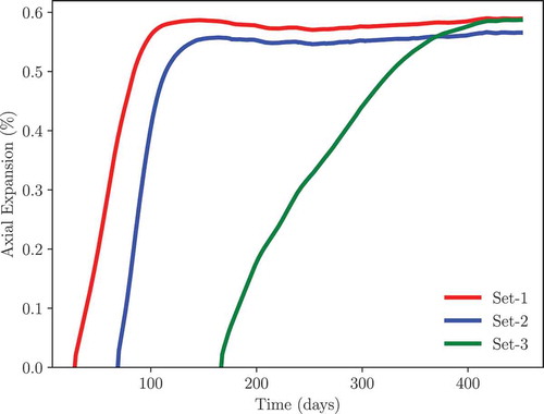
As noted by Ref. 58, the start time of the experiment can significantly affect the ASR expansion behavior because of the effects of synchronizing the aging of the concrete with the periods of high temperature when ASR expansion is accelerated. To illustrate the effect of starting the same experiment at different times of the year, the same unreinforced concrete block was simulated with three different starting times for exposure to the environmental conditions. The start time of exposure of the block to the temperature and relative humidity history shown in Fig. 10 is varied to match the times used for the three sets of experiments conducted by Ref. 58. Here, Set-1 corresponds to the concrete (Specimen A1-000b) expansion as reported by Ref. 58 that is used for calibrating the ASR model in BlackBear. Set-2 and Set-3 concretes are considered to have been cast at later times and their testing started approximately from 69 days and 166 days, respectively. Similar dependencies on start time were shown by Ref. 58, but for specimens with varying reinforcement configurations because unreinforced blocks were not actually tested at each of these start times. It is advantageous, however, to compare the response of identical unreinforced blocks to highlight the effects of environmental conditions on ASR kinetics. The results of this parameter study shown in Fig. 12 clearly demonstrate that starting at a time with a lower temperature impedes the ASR reaction and delays its onset.

Fig. 12. BlackBear simulation results showing the effect of the environmental conditions on the free expansion of a plain concrete block. Here, the exposure of the block to the temperature and relative humidity history varies with the start time

The same set of parameters calibrated for the unreinforced block was then applied to predict the expansion of the reinforced concrete block. Figure 13 compares the contours of the local volumetric expansion of the concrete block with no reinforcement (Specimen A1-000b) and with uniaxial reinforcement (Specimen A1-001a from Ref. 58) at the end of the experiment. As can be seen in Fig. 13, the presence of rebar constrains the expansion in the axial direction of the bars. It can also be seen that the volumetric expansion is slightly lower along the edges of both blocks, which can be attributed to the relative humidity being lower in the early stages of the experiment because it more closely tracked the environmental conditions.

Fig. 13. Volumetric expansion of a concrete block with (a) no reinforcement (Specimen A1-000b) and (b) with uniaxial reinforcement (Specimen A1-001a). The deformation is magnified 50$\times$ to highlight the confining effect of the bars

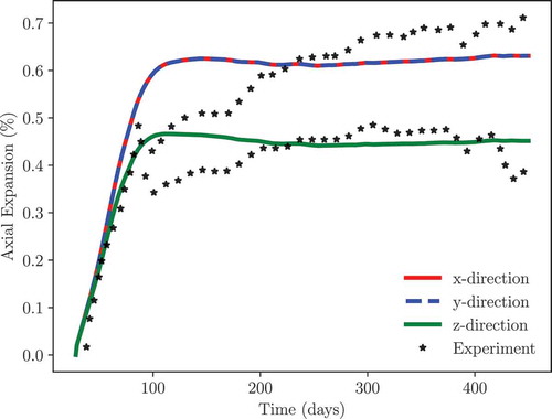
Time histories of the simulated average axial expansion in the three directions are shown compared with experimental results in Fig. 14. The constraining effect of the rebar in the z-direction is clearly evident as a decreased expansion in that direction relative to the other two directions. In this scenario, the expansion in the x- and y-directions are nearly identical and overlay each other. It should be noted that although the damage model is active in all of these cases, the numerical models did not predict the onset of any damage. ASR expansion is over predicted in all directions early in the aging process, but eventually approaches experimental results. Similar behavior is observed for the unreinforced block (Fig. 11). This may be due to issues inherent in the ASR expansion or isotropic damage models used here.

Fig. 14. Experimental and simulation results for axial expansion of a concrete block with uniaxial reinforcement (Specimen A1-001a) showing the effect of reinforcement on the response in the three directions

V. SUMMARY AND FUTURE WORK

The Grizzly and BlackBear codes utilize the capabilities of the MOOSE framework to understand the effects of aging on structural components in nuclear power plants and can also be used to address such phenomena in other similar structures used for other applications as well. There is a wide variety of structures in a nuclear power plant, and the development work in these codes to date has primarily focused on the RPV and reinforced concrete capabilities described here. These have both reached the point where they are largely feature complete, and the emphasis has shifted from development to testing of these capabilities. Representative simulations of an RPV and a concrete specimen have been presented here.

There are still some important limitations to the capabilities shown here. For RPV modeling, one important area where further development is needed is in a capability to compute not only the probability of crack initiation, but of crack propagation through the RPV wall. This involves the development of an initiation, growth, and arrest model, which has been prototyped but still needs further development. For reinforced concrete, a comprehensive capability requires robust capabilities to model nonlinear mechanical behavior, including damage and rebar bond slip. Some capability exists in this area, but this is another area of active development and testing.

A significant current emphasis is on the testing of the RPV capabilities. Because of the nature of the RPV problem, it is difficult to validate PFM calculations against experimental data. However, multiple aspects of these models (such as thermal and mechanical response and fracture-mechanics solutions) can be verified against known mathematical solutions. In addition, the PFM predictions can be benchmarked against solutions from other codes. A summary of a recent effort in which Grizzly’s PFM calculations were benchmarked against another code using 1-D models to represent the global behavior is provided in Ref. 60 and shows generally good agreement across a range of conditions. PFM predictions such as those presented in this paper are highly sensitive to the input parameters, and a thorough investigation of the sensitivity to the various parameters is warranted. As previously mentioned, CFD simulations could be readily coupled with the 3-D PFM models described here to better understand the effects of the cold plume under more realistic conditions. Also, development of lower-length-scale predictive models of RPV steel microstructure and property evolution is ongoing, with the goal of developing a predictive model of embrittlement that can be confidently applied for long-term operation scenarios.

For concrete, a growing body of experimental data is available for validation of the simulation models, and work is underway to develop a suite of problems that simulate those data. The case shown in this paper is part of a larger suite of problems, the development of which is documented in Ref. 60. In addition, extensive data are available on the nonlinear response of reinforced concrete structures to mechanical loading. Validation against those data is also important to ensure that the code adequately predicts this behavior. Once confidence has been developed in the ability of the code to predict ASR expansion and nonlinear mechanical response, the validation test suite will also be expanded to include predictions of the behavior of ASR-affected structures subjected to mechanical loading. These codes will also be applied to the simulation of full-scale nuclear structures. The concrete simulation framework is reasonably complete at this point, but as testing and application reviews limitations with the current set of models, these models will be revised accordingly.

The discussion here has focused on two important classes of LWR structural systems, but there are many other important systems to consider as well. In LWRs, stress corrosion cracking in core internal structures and other components in contact with the coolant loop are a high priority for future development. A framework for predictive modeling of high-temperature creep response in advanced reactor alloys is being developed. Modeling the response of graphite reflectors is also of interest for advanced reactor applications. The coupled physics simulation capabilities of the MOOSE framework will greatly facilitate the development of simulation tools for these applications, and many of the foundational capabilities used here will also be useful for these other applications. Finally, it should be emphasized that the intent of this effort is to make these capabilities widely available to the nuclear industry. This is being done by making BlackBear available to the general public as an open-source code and by making Grizzly readily available, with export control restrictions, through INL’s standard code access channels.

Acknowledgments

This work was funded by the DOE’s Office of Nuclear Energy’s Modeling and Simulation and LWRS programs. This paper has been authored by a contractor of the U.S. Government under contract DE-AC07-05ID14517. Accordingly, the U.S. Government retains a nonexclusive, royalty free license to publish or reproduce the published form of this contribution, or allow others to do so, for U.S. Government purposes.

References

- S. ZINKLE and G. WAS, “Materials Challenges in Nuclear Energy,” Acta Mater., 61, 3, 735 (2013); https://doi.org/10.1016/j.actamat.2012.11.004.
- “NRC Datasets,” U.S. Nuclear Regulatory Commission (2020).
- “Status of Subsequent License Renewal Applications,” U.S. Nuclear Regulatory Commission; https://www.nrc.gov/reactors/operating/licensing/renewal/subsequent-license-renewal.html ( current as of July 10, 2020).
- “Light Water Reactor Sustainability Program: Integrated Program Plan,” INL/EXT-11-23452, Rev 4, Idaho National Laboratory (2016).
- H. D. GOUGAR, “High Temperature Reactor Research and Development Roadmap, Draft for Public Comment,” INL/EXT-17-41803, Rev 3, Idaho National Laboratory (2017).
- G. WAS et al., “Materials for Future Nuclear Energy Systems,” J. Nucl. Mater., 527, 151837 (2019); https://doi.org/10.1016/j.jnucmat.2019.151837.
- C. J. PERMANN et al., “MOOSE: Enabling Massively Parallel Multiphysics Simulation,” SoftwareX, 11, 100430 (2020); https://doi.org/10.1016/j.softx.2020.100430.
- R. K. NANSTAD et al., “Expanded Materials Degradation Assessment (EMDA) Volume 3: Aging of Reactor Pressure Vessels,” NUREG/CR-7153, Vol. 3, ORNL/TM-2013/532, Oak Ridge National Laboratory (2014).
- H. GRAVES et al., “Expanded Materials Degradation Assessment (EMDA) Volume 4: Aging of Concrete and Civil Structures,” NUREG/CR-7153, Vol. 4, ORNL/TM-2013/532, Oak Ridge National Laboratory (2014).
- E. EASON et al., “A Physically-Based Correlation of Irradiation-Induced Transition Temperature Shifts for RPV Steels,” J. Nucl. Mater., 433, 1–3, 240 (2013); https://doi.org/10.1016/j.jnucmat.2012.09.012.
- Y. ZHANG et al., “Formation of Prismatic Loops from C15 Laves Phase Interstitial Clusters in Body-Centered Cubic Iron,” Scr. Mater., 98, 5 (2015); https://doi.org/10.1016/j.scriptamat.2014.10.033.
- Y. ZHANG et al., “Preferential Cu Precipitation at Extended Defects in BCC Fe: An Atomistic Study,” Comput. Mater. Sci, 101, 181 (2015); https://doi.org/10.1016/j.commatsci.2015.01.041.
- X.-M. BAI et al., “Modeling Copper Precipitation Hardening and Embrittlement in a Dilute Fe-0.3at.%Cu Alloy Under Neutron Irradiation,” J. Nucl. Mater., 495, 442 (2017); https://doi.org/10.1016/j.jnucmat.2017.08.042.
- P. CHAKRABORTY and S. B. BINER, “Parametric Study of Irradiation Effects on the Ductile Damage and Flow Stress Behavior in Ferritic-Martensitic Steels,” J. Nucl. Mater., 465, 89 (2015); https://doi.org/10.1016/j.jnucmat.2015.05.054.
- P. CHAKRABORTY and S. B. BINER, “Crystal Plasticity Modeling of Irradiation Effects on Flow Stress in Pure-Iron and Iron-Copper Alloys,” Mech. Mater., 101, 71 (2016); https://doi.org/10.1016/j.mechmat.2016.07.013.
- P. CHAKRABORTY and S. B. BINER, “A Unified Cohesive Zone Approach to Model the Ductile to Brittle Transition of Fracture Toughness in Reactor Pressure Vessel Steels,” Eng. Fract. Mech., 131, 194 (2014); https://doi.org/10.1016/j.engfracmech.2014.07.029.
- Y. ZHANG et al., “Mesoscale Modeling of Solute Precipitation and Radiation Damage,” INL/EXT-15-36754, Idaho National Laboratory (2015).
- “BlackBear Source Code Repository,” https://github.com/idaholab/blackbear ( current as of July 10, 2020).
- R. L. WILLIAMSON et al., “BISON: A Flexible Code for Advanced Simulation of the Performance of Multiple Nuclear Fuel Forms,” Nucl. Technol., 207, 954 (2021); https://doi.org/10.1080/00295450.2020.1836940.
- S. NOVASCONE et al., “Evaluation of Coupling Approaches for Thermomechanical Simulations,” Nucl. Eng. Des., 295, 910 (2015); https://doi.org/10.1016/j.nucengdes.2015.07.005.
- T. BELYTSCHKO and T. BLACK, “Elastic Crack Growth in Finite Elements with Minimal Remeshing,” Int. J. Numer. Methods Eng., 45, 5, 601 (1999); https://doi.org/10.1002/(SICI)1097-0207(19990620)45:5<601::AID-NME598>3.0.CO;2-S.
- N. MOËS, J. DOLBOW, and T. BELYTSCHKO, “A Finite Element Method for Crack Growth Without Remeshing,” Int. J. Numer. Methods Eng., 46, 1, 131 (1999); https://doi.org/10.1002/(SICI)1097-0207(19990910)46:1<131::AID-NME726>3.0.CO;2-J.
- A. HANSBO and P. HANSBO, “A Finite Element Method for the Simulation of Strong and Weak Discontinuities in Solid Mechanics,” Comput. Methods Appl. Mech. Eng., 193, 33–35, 3523 (2004); https://doi.org/10.1016/j.cma.2003.12.041.
- W. JIANG, B. W. SPENCER, and J. E. DOLBOW, “Ceramic Nuclear Fuel Fracture Modeling with the Extended Finite Element Method,” Eng. Fract. Mech., 223, 106713 (2020); https://doi.org/10.1016/j.engfracmech.2019.106713.
- M. C. WALTERS, G. H. PAULINO, and R. H. DODDS, “Interaction Integral Procedures for 3-D Curved Cracks Including Surface Tractions,” Eng. Fract. Mech., 72, 11, 1635 (2005); https://doi.org/10.1016/j.engfracmech.2005.01.002.
- Irradiation Embrittlement of Reactor Pressure Vessels (RPVS) in Nuclear Power Plants, No. 26 in Woodhead Publishing Series in Energy, N. SONEDA, Ed., Woodhead Publishing, Waltham, Massachusetts (2015).
- K. THAMARAISELVI and S. VISHNUVARDHAN, “Fracture Studies on Reactor Pressure Vessel Subjected to Pressurised Thermal Shock: A Review,” Nucl. Eng. Des., 360, 110471 (2020); https://doi.org/10.1016/j.nucengdes.2019.110471.
- G. QIAN and M. NIFFENEGGER, “Procedures, Methods and Computer Codes for the Probabilistic Assessment of Reactor Pressure Vessels Subjected to Pressurized Thermal Shocks,” Nucl. Eng. Des., 258, 35 (2013); https://doi.org/10.1016/j.nucengdes.2013.01.030.
- K. ONIZAWA, H. NISHIKAWA, and H. ITOH, “Development of Probabilistic Fracture Mechanics Analysis Codes for Reactor Pressure Vessels and Piping Considering Welding Residual Stress,” Int. J. Press. Vessels Pip., 87, 1, 2 (2010); https://doi.org/10.1016/j.ijpvp.2009.11.011.
- P. WILLIAMS et al., “Fracture Analysis of Vessels – Oak Ridge, FAVOR, V16.1, Computer Code: Theory and Implementation of Algorithms, Methods, and Correlations,” ORNL/LTR-2016/309, Oak Ridge National Laboratory (2016).
- B. W. SPENCER et al., “Coupling of Neutron Transport and Probabilistic Fracture Mechanics Codes for Analysis of Embrittled Reactor Pressure Vessels,” ASME Pressure Vessels and Piping Conf., PVP2020–21680, American Society of Mechanical Engineers, Virtual Online, August 3, 2020.
- B. SPENCER, W. HOFFMAN, and M. BACKMAN, “Modular System for Probabilistic Fracture Mechanics Analysis of Embrittled Reactor Pressure Vessels in the Grizzly Code,” Nucl. Eng. Des., 341, 25 (2019); https://doi.org/10.1016/j.nucengdes.2018.10.015.
- G. J. SCHUSTER et al., “Characterization of Flaws in U.S. Reactor Pressure Vessels,” NUREG/CR-6741, Vol. 2, PNNL-11143B, Pacific Northwest National Laboratory (2000).
- H. F. BÜCKNER, “A Novel Principle for the Computation of Stress Intensity Factors,” Z. Angew Math. Mech., 50, 529 (1970).
- “ASME Boiler and Pressure Vessel Code, Section XI, Rules for Inservice Inspection of Nuclear Power Plant Components,” ASME BPVC.XI-2017, American Society of Mechanical Engineers (2017).
- R. C. CIPOLLA, “Computational Method to Perform the Flaw Evaluation Procedure as Specified in the ASME Code, Section XI, Appendix A,” EPRI Report NP-1181, Failure Analysis Associates (1979).
- G. QIAN et al., “Effect of Non-Uniform Reactor Cooling on Fracture and Constraint of a Reactor Pressure Vessel,” Fatigue Fract. Eng. Mater. Struct., 41, 7, 1559 (2018); https://doi.org/10.1111/ffe.12796.
- H. UITSLAG-DOOLAARD et al., “Numerical Prediction of a Single Phase Pressurized Thermal Shock Scenario for Crack Assessment in a Reactor Pressure Vessel Wall,” Ann. Nucl. Energy, 144, 107563 (2020); https://doi.org/10.1016/j.anucene.2020.107563.
- “Regulatory Guide 1.99: Radiation Embrittlement of Reactor Vessel Materials, Revision 2,” U.S. Nuclear Regulatory Commission (1988).
- F.-J. ULM et al., “Thermo-Chemo-Mechanics of ASR Expansion in Concrete Structures,” J. Eng. Mech., 126, 3, 233 (2000); https://doi.org/10.1061/(ASCE)0733-9399(2000)126:3(233).
- V. SAOUMA, L. PEROTTI, and T. SHIMPO, “Stress Analysis of Concrete Structures Subjected to Alkali-Aggregate Reactions,” ACI Struct. J., 104, 5, 532 (2007).
- L. JASON et al., “Hydraulic Behaviour of a Representative Structural Volume for Containment Buildings,” Nucl. Eng. Des., 237, 12–13, 1259 (2007); https://doi.org/10.1016/j.nucengdes.2006.09.035.
- S. MULTON and A. SELLIER, “Multi-Scale Analysis of Alkali-Silica Reaction (ASR): Impact of Alkali Leaching on Scale Effects Affecting Expansion Tests,” Cem. Concr. Res., 81, 122 (2016); https://doi.org/10.1016/j.cemconres.2015.12.007.
- M. S. POURBEHI, G. P. VAN ZIJL, and J. STRASHEIM, “Analysis of Combined Action of Seismic Loads and Alkali-Silica Reaction in Concrete Dams Considering the Key Chemical-Physical-Mechanical Factors and Fluid-Structure Interaction,” Eng. Struct., 195, 263 (2019); https://doi.org/10.1016/j.engstruct.2019.05.087.
- D.-M. BOUHJITI et al., “Accounting for Realistic Thermo-Hydro-Mechanical Boundary Conditions Whilst Modeling the Ageing of Concrete in Nuclear Containment Buildings: Model Validation and Sensitivity Analysis,” Eng. Struct., 166, 314 (2018); https://doi.org/10.1016/j.engstruct.2018.03.015.
- “NRC Information Notice 2011-20: Concrete Degradation by Alkali-Silica Reaction,” U.S. Nuclear Regulatory Commission (Nov. 18, 2011).
- T. M. ROSSEEL et al., “Review of the Current State of Knowledge on the Effects of Radiation on Concrete,” J. Adv. Concr. Technol., 14, 7, 368 (2016); https://doi.org/10.3151/jact.14.368.
- H. HUANG, B. W. SPENCER, and G. CAI, “Grizzly Model of Multi-Species Reactive Diffusion, Moisture/Heat Transfer and Alkali-Silica Reaction in Concrete,” INL/EXT-15-36425, Idaho National Laboratory (2015).
- R. BALLARINI et al., “Multiple Degradation Mechanisms in Reinforced Concrete Structures, Modeling and Risk Analysis,” INL/EXT-20-57095, Idaho National Laboratory (2020).
- Z. P. BAŽANT, J.-C. CHERN, and W. THONGUTHAI, “Finite Element Program for Moisture and Heat Transfer in Heated Concrete,” Nucl. Eng. Des., 68, 1, 61 (1982); https://doi.org/10.1016/0029-5493(82)90040-1.
- V. SAOUMA et al., “Structural Significance of Alkali-Silica Reaction in Massive Reinforced Concrete Structures,” ORNL/TM-2014/489, Oak Ridge National Laboratory (2014).
- ASCE COMMITTEE ON FIRE PROTECTION, Structural Fire Protection, American Society of Civil Engineers, New York (1992).
- V. KODUR, T. WANG, and F. CHENG, “Predicting the Fire Resistance Behaviour of High Strength Concrete Columns,” Cem. Concr. Compos., 26, 2, 141 (2004); https://doi.org/10.1016/S0958-9465(03)00089-1.
- EUROCODE, Design of Concrete Structures. Part 1-2: General Rules - Structural Fire Design, European Committee for Standardization, Brussels, Belgium (2004).
- V. SAOUMA and L. PEROTTI, “Constitutive Model for Alkali-Aggregate Reactions,” ACI Mater. J., 103, 3 (2006); https://doi.org/10.14359/15853.
- A. B. GIORLA, “Simulation of Concrete Members Affected by Alkali-Silica Reaction with Grizzly,” ORNL/TM-2016/523, Oak Ridge National Laboratory (2016).
- C. F. DUNANT and K. L. SCRIVENER, “Effects of Uniaxial Stress on Alkali-Silica Reaction Induced Expansion of Concrete,” Cem. Concr. Res., 42, 3, 567 (2012); https://doi.org/10.1016/j.cemconres.2011.12.004.
- D. M. WALD et al., “Development and Multiaxial Distribution of Expansions in Reinforced Concrete Elements Affected by Alkali-Silica Reaction,” Struct. Concr., 18, 914 (2017); https://doi.org/10.1002/suco.201600220.
- B. W. SPENCER and H. HUANG, “Coupled Physics Simulation of Expansive Reactions in Concrete with the Grizzly Code,” Proc. 18th Int. Conf. on Environmental Degradation of Materials in Nuclear Power Systems—Water Reactors, J. H. JACKSON, D. PARAVENTI, and M. WRIGHT Eds., pp. 131–141, Springer (2017).
- B. W. SPENCER et al., “Assessment of Grizzly Capabilities for Reactor Pressure Vessels and Reinforced Concrete Structures,” INL/EXT-20-59941, Idaho National Laboratory (2020).