Method of Characteristics for 3D, Full-Core Neutron Transport on Unstructured Mesh

Abstract

A myriad of nuclear reactor designs are currently being considered for next-generation power production. These designs utilize unique geometries and materials and can rely on multiphysics effects for safety and operation. This work develops a neutron transport tool, MOCkingbird, capable of three-dimensional (3D), full-core reactor simulation for previously intractable geometries. The solver is based on the method of characteristics, utilizing unstructured mesh for the geometric description. MOCkingbird is built using the MOOSE multiphysics framework, allowing for straightforward linking to other physics in the future. A description of the algorithms and implementation is given, and solutions are computed for two-dimensional/3D C5G7 and the Massachusetts Institute of Technology BEAVRS benchmark. The final result shows the application of MOCkingbird to a 3D, full-core simulation utilizing 1.4 billion elements and solved using 12 000 processors.

Keywords:

• Method of characteristics
• unstructured mesh
• MOCkingbird
• MOOSE, BEAVRS

I. INTRODUCTION

Modeling and simulation of nuclear reactors play a vital role in their life cycle. The existing fleet has relied heavily on modeling and simulation based on informed approximations from many experiments and decades of operating experience. The existing tools have proven themselves to be up to the task for simulation of existing reactor designs. These tools have heavily relied on nodal calculations,^1–3 with support from two-dimensional (2D) method of characteristics (MOC) solvers for lattice calculations.^4–7 However, most designs among the next generation of advanced reactors would benefit from three-dimensional (3D), full-core, neutron transport calculations. One of the primary drivers for this is the need to be agnostic to model complex, heterogeneous axial geometry. In addition, multiphysics effects, such as core “flowering” in sodium-cooled fast reactors,⁸ can also be captured using flexible 3D neutron transport tools. Unfortunately, high-fidelity, 3D neutron transport calculation has largely remained on the sidelines due to large computational requirements.⁹ Recently, groundbreaking research in 3D, full-core, neutron transport has led to some of the first viable solution methods for reactor design.^9–15

This work develops a MOC neutron transport method on unstructured mesh that is accurate, scalable, geometrically flexible, capable of full-core 3D calculation, and able to respond to arbitrary multiphysics interactions, such as geometric deformation. To achieve these goals, a new neutron transport solver, named MOCkingbird, was developed utilizing the MOOSE framework.^16,17 MOOSE provides MOCkingbird with the underlying geometrical representation and a simplified linking to other physics within the reactor core. Utilizing unique algorithms for parallelization of MOC, MOCkingbird can efficiently solve both 2D and 3D neutron transport problems.

This paper is composed as follows: Sec. II presents the state of the art of the underlying numerical method in MOCkingbird, the MOC, and its use with unstructured mesh. Section III summarizes the main advanced features of MOCkingbird, while Sec. IV dives into some of the fundamentals of the method and presents some of the technical choices made during implementation. Finally, Sec. V presents numerical light water reactor benchmarks solved with MOCkingbird, providing both validation and an evaluation of its scaling and performance.

II. BACKGROUND

II.A. MOC for Neutron Transport

Transport simulations can predict the flow of neutrons through materials, enabling predictive modeling of radiation shielding, neutron detectors, critical experiments, and reactor cores. The MOC, further described in Sec. IV, is a solution method that is used in many fields and has seen broad adoption in the nuclear engineering community for solving the neutron transport equation, starting from the work of Ref. 18. MOC has become broadly used in reactor analysis, supplanting other transport solution methodologies for many applications, including lattice physics.¹⁹

The MOC is traditionally solved using constructive solid geometry^20,21 (CSG). CSG represents the surfaces within a reactor using a parametric representation of simple shapes, which are then operated on with Boolean logic. This scheme has been particularly successful for modeling light water reactors due to its ability to perfectly represent the concentric cylinders placed within lattices inherent to that geometry. Early efforts successfully utilized MOC for cross-section and discontinuity factor calculations for input into full-core nodal calculations.^2,4 Extensive research utilizing this method for 2D radial calculations has led to efficient, accelerated,^22,23 parallel^20,21,24 codes capable of full-core calculations.²⁵ Lately, breakthrough work has led to some of the first 3D, full-core MOC calculations.^9–12 In the last 15 years, considerable work has been done to successfully leverage axial couplings of 2D MOC solutions, in what is known as 2D/one-dimensional (1D) transport,^26,27 to provide 3D transport solutions at lower cost and accuracy than 3D MOC.

II.B. Unstructured Mesh MOC State of the Art

While CSG is ideal for ray tracing, it can be difficult to use for representing complicated geometries and geometric deformation.²⁸ An alternative is unstructured mesh. Most commonly used in finite element solvers, unstructured mesh builds geometry out of discrete “elements” that are made of simple shapes such as triangles, quadrilaterals, hexahedra, and tetrahedra. Many of these small elements can be combined to create complicated geometries that can then be straightforwardly deformed. This is the approach MOCkingbird uses for geometrical representation. In addition to the flexibility gained through utilizing unstructured mesh, by abstracting ray tracing to be across an element, MOCkingbird gains the ability to work in 1D, 2D, and 3D. Unstructured mesh is also the basis for numerous non-MOC finite element transport solvers.^29,30

Utilization of unstructured mesh as the geometric representation for MOC is not, in itself, a new concept. Several previous studies have applied this methodology. Two of the most successful implementations of MOC utilizing unstructured mesh were developed at Argonne National Laboratory: MOCFE (Ref. 31) and PROTEUS-MOCEX (Ref. 32). While these two codes share a similar geometric discretization, including the ability to solve 3D, they vary greatly in implementation detail.

Of paramount importance to MOC on unstructured mesh is the ability to handle communication of angular flux moments across domain decomposed geometry. In light of this, MOCFE utilized a novel matrix-free generalized minimum residual method (GMRES) solver to accelerate a nonimplicit global sweep iterative algorithm. To further reduce parallel communication due to domain decomposition, MOCFE also employed angle- and energy-based decomposition. MOCFE utilized a distributed-mesh back-projection³³ (among other schemes) to generate 3D trajectories (trajectories out of the radial plane) allowing for MOC solutions in 3D geometries. Ghosting for track generation and load balancing for the computationally expensive solution phase were explored. The back-projection of the geometry being different for each angle proved challenging for load balancing.

PROTEUS-MOCEX utilized a wholly different scheme for the solution of 3D transport problems. Instead of directly generating 3D trajectories, PROTEUS-MOCEX built on the extensive research into so-called 2D/1D methods that utilize CSG (Refs. 34 and 35). Broadly, 2D/1D methods employ transport solvers (such as MOC) in the radial direction and lower-order methods in the axial direction (such as diffusion, or S_N). This scheme can be incredibly effective due to reactors often having much higher geometric and material variability in the radial direction than the axial direction. PROTEUS-MOCEX, in addition to utilizing unstructured mesh, went one step further: It replaced the 1D axial solve and the axial leakage term in 2D with a 1D finite element treatment and effectively 3D sources in the 2D MOC solve.³² The 2D MOC sweep was then coupled into the axial solve as a line source. This provided the efficiency needed to solve complex 3D transport problems.³⁶

Several other research efforts have also utilized unstructured mesh with MOC. The MOC on Unstructured Mesh³⁷ (MOCUM) project is heavily focused on automatically converting CSG geometry into triangular elements. A Delaunay triangulation algorithm was created, allowing for simplified workflow from reactor geometry discretization to MOC solution. Parallelism in MOCUM was handled using OpenMP. MoCha-Foam³⁸ was developed using the OpenFoam open-source, partial differential equation (PDE) solver framework, allowing for future expansion into multiphysics problems. Finally, an effort to utilize linear source representation on unstructured meshes³⁹ was undertaken at Bhabha Atomic Research Center in Mumbai. Similar to MOCUM, a triangulation was utilized to produce the geometry, however, less elements were needed due to the higher-order representation of the source. One unique aspect of this effort was that it utilized curved triangle edges to reduce geometric representation error.

Each of these research efforts pushed the state of the art forward for MOC on unstructured mesh. However, many aspects still remain unsolved. These include accurate reflective boundary condition treatment,^31,40 memory issues,³² parallelization,^33,37,38 and parallel track generation.³³ This project aims to alleviate these issues through the development of MOCkingbird.

III. MOCkingbird

MOCkingbird has been developed using MOOSE, which is a framework for building multiphysics tools, and therefore is a natural fit for a code that will ultimately perform multiphysics analysis of reactors. MOOSE provides important infrastructure to MOCkingbird, including finite element mesh, ray-tracing capabilities, input/output, online post processing, auxiliary field computations, code timing, memory management, testing infrastructure, and straight-forward coupling to other MOOSE-based applications.

The other significant library dependency is that of OpenMOC, which MOCkingbird relies on for track generation.⁴⁰ OpenMOC contains routines for the efficient generation of cyclic 2D and 3D tracks. The ability to selectively generate 3D tracks based on a unique one dimension is critical to efficient track generation and claiming. In addition, said track generation also computes the necessary quadrature weights to use with the tracks for angular and spatial integration.

III.A. Summary of Main Features

MOCkingbird uses the conventional flat source MOC formulation as detailed in Ref. 19. Long characteristic tracks (domain boundary to domain boundary) are used in both serial and parallel, providing the same solver behavior regardless of the number of message passing interface⁴¹ (MPI) ranks used. At this time, MOCkingbird uses flat source, isotropic scattering, isotropic fission source, and multigroup cross-section approximations. MOCkingbird does not contain cross-section generation capabilities; thus, all cross sections must be generated externally. However, a flexible interface exists to allow for the reading of many different types of cross-section databases. One in-progress aspect of MOCkingbird is its acceleration capability based on DSA,²³ rather than CMFD,^22,42 which is more commonly used in MOC programs. Acceleration in MOCkingbird is still under heavy development and will be the subject of future publications.

Some interesting or unique aspects of MOCkingbird are

1. unstructured mesh for geometry definition and spatial discretization

2. no geometric assumptions made in the solver

3. capable of working with moving mesh, e.g., from thermal expansion or fracture

4. same solution behavior in serial and parallel

5. parallel, scalable cyclic track generation, starting point location, and track distribution

6. asynchronous sparse data exchange algorithms during problem setup

7. scalable communication routines during problem setup

8. efficient, robust element traversal

9. scalable, domain decomposed ray tracing

10. smart buffering for messages

11. scalable memory usage

12. object pool utilization to reduce memory allocation and deallocation

13. weighted partitioning for load balance

14. high parallel scalability

15. developed using MOOSE for simplified linking to other physics codes.

III.B. Ray-Tracing Capabilities

Asynchronous parallel ray tracing allows for the integration of a complete track across the entire domain decomposed geometry without any intermediate global synchronization or iteration. This sets apart MOCkingbird from other MOC codes and aids in convergence. Because such a capability could be useful for solving many physical problems, e.g., radiative heat transfer or shock waves, MOCkingbird’s ray-tracing capability has been abstracted into a MOOSE module that will be part of the open source release in the near future. The details of this parallel algorithm are beyond the scope of the current discussion and will be detailed in a future publication.

As is mentioned in Sec. IV.E, many MOC codes employ modular ray tracing (MRT) and modular spatial domain decomposition (SDD) (Refs. 9 and 43) in parallel. When using a modular decomposition, tracks are only integrated from one partition boundary to another within one source iteration, creating a block-Jacobi-like method. As noted in Ref. 33, this idea is untenable for arbitrarily decomposed unstructured mesh that is partitioned with a mesh partitioner.

Figure 1 shows why this is the case. With unstructured-mesh partitioning there are many jagged/reentrant corners along partition boundaries. If a track were to pass through the domain in such a way that it follows a partition boundary, then a block-Jacobi-like tracing of that track would take many source iterations before boundary information is propagated across the domain.⁹ In a large 3D mesh for a full reactor core with millions of tracks, this situation frequently occurs. Similar issues have been studied for the domain decomposition of discrete ordinates sweeps in finite element neutron transport.^44,45

Fig. 1. The mesh is split for three MPI ranks, and one track is considered. With a block-Jacobi-like algorithm, the boundary angular flux would only propagate to the other side of the domain after all source iterations. In MOCkingbird, the entire track is traced in one iteration without any intermediate global synchronization

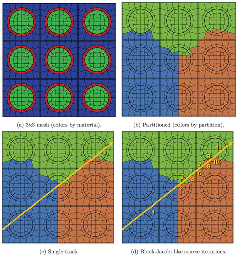
Utilizing an asynchronous communication strategy, MOCkingbird efficiently traces the track shown in Fig. 1c in one source iteration without any intermediate global synchronization. This provides multiple advantages: behavior is the same in parallel and serial, storage of partition angular fluxes is not required (therefore scalable in memory), and the convergence rate is not reduced as observed in Ref. 9.

IV. MOC IN MOCkingbird

The MOCkingbird code utilizes a traditional form of MOC that makes use of flat spatial source regions and transport-corrected-P₀ scattering cross sections. These simplifications can be removed in the future, but provide a good basis to start from. Many detailed treatments of this formulation are found in the literature.^4,9,20,43,46

This section gives an overview of the characteristic form of the steady-state Boltzmann neutron transport equation as used by MOCkingbird. Sections IV.A through IV.F start from the multigroup, isotropic scattering approximation and review the reduction to a problem that is discrete in both angle and space. Ultimately, a source iteration scheme is developed for the iterative solution of the k-eigenvalue problem.⁴⁷

IV.A. Characteristic Equation

We start from the isotropic scattering multigroup neutron multiplication eigenproblem, the derivation of which can be found in any reactor physics book, e.g., Ref. 48. This equation reads:

$\begin{array}{rl}& \left(\mathbf{\Omega }\cdot \mathrm{\nabla }+{\mathrm{\Sigma }}_{t,g}(\mathit{r})\right){\psi }_g(\mathit{r},\mathbf{\Omega })\\ & =\frac{1}{4\pi }\sum _{g{ }^{\mathrm{\prime }}=1,n_g}{\int }_{4\pi }{\mathrm{\Sigma }}_{s0,g{ }^{\mathrm{\prime }}\to g}(\mathit{r}){\psi }_{g{ }^{\mathrm{\prime }}}(\mathit{r},{\mathbf{\Omega }}^{\prime }){\mathrm{d}\mathbf{\Omega }}^{\prime }+\frac{{\chi }_g(\mathit{r})}{4\pi k_{eff}}\\ & \sum _{g{ }^{\mathrm{\prime }}=1,n_g}{\int }_{4\pi }\nu {\mathrm{\Sigma }}_{f,g{ }^{\mathrm{\prime }}}(\mathit{r}){\psi }_{g{ }^{\mathrm{\prime }}}(\mathit{r},{\mathbf{\Omega }}^{\prime }){\mathrm{d}\mathbf{\Omega }}^{\prime }.(1)\end{array}$

Equation (1)$\begin{array}{rl}& \left(\mathbf{\Omega }\cdot \mathrm{\nabla }+{\mathrm{\Sigma }}_{t,g}(\mathit{r})\right){\psi }_g(\mathit{r},\mathbf{\Omega })\\ & =\frac{1}{4\pi }\sum _{g{ }^{\mathrm{\prime }}=1,n_g}{\int }_{4\pi }{\mathrm{\Sigma }}_{s0,g{ }^{\mathrm{\prime }}\to g}(\mathit{r}){\psi }_{g{ }^{\mathrm{\prime }}}(\mathit{r},{\mathbf{\Omega }}^{\prime }){\mathrm{d}\mathbf{\Omega }}^{\prime }+\frac{{\chi }_g(\mathit{r})}{4\pi k_{eff}}\\ & \sum _{g{ }^{\mathrm{\prime }}=1,n_g}{\int }_{4\pi }\nu {\mathrm{\Sigma }}_{f,g{ }^{\mathrm{\prime }}}(\mathit{r}){\psi }_{g{ }^{\mathrm{\prime }}}(\mathit{r},{\mathbf{\Omega }}^{\prime }){\mathrm{d}\mathbf{\Omega }}^{\prime }.(1)\end{array}$ represents a balance between production and loss of neutrons, with the fundamental eigenvalue k_eff balancing the system that might otherwise not have a steady state. The groupwise angular fluxes ${\psi }_g$ are the dependent variables in Eq. (1)$\begin{array}{rl}& \left(\mathbf{\Omega }\cdot \mathrm{\nabla }+{\mathrm{\Sigma }}_{t,g}(\mathit{r})\right){\psi }_g(\mathit{r},\mathbf{\Omega })\\ & =\frac{1}{4\pi }\sum _{g{ }^{\mathrm{\prime }}=1,n_g}{\int }_{4\pi }{\mathrm{\Sigma }}_{s0,g{ }^{\mathrm{\prime }}\to g}(\mathit{r}){\psi }_{g{ }^{\mathrm{\prime }}}(\mathit{r},{\mathbf{\Omega }}^{\prime }){\mathrm{d}\mathbf{\Omega }}^{\prime }+\frac{{\chi }_g(\mathit{r})}{4\pi k_{eff}}\\ & \sum _{g{ }^{\mathrm{\prime }}=1,n_g}{\int }_{4\pi }\nu {\mathrm{\Sigma }}_{f,g{ }^{\mathrm{\prime }}}(\mathit{r}){\psi }_{g{ }^{\mathrm{\prime }}}(\mathit{r},{\mathbf{\Omega }}^{\prime }){\mathrm{d}\mathbf{\Omega }}^{\prime }.(1)\end{array}$. Solving for ${\psi }_g$ allows for the computation of reaction rates throughout the core. ${\mathrm{\Sigma }}_{t,g}$, ${\mathrm{\Sigma }}_{s0,g{ }^{\mathrm{\prime }}\to g}$, and $\nu {\mathrm{\Sigma }}_{f,g}$ are the groupwise total, scatter, and nu-fission macroscopic cross sections, respectively. A position in 3D space is denoted by $\mathit{r}$. The direction of neutron travel is represented by $\mathbf{\Omega }$, a point on the unit sphere in ${\mathbb{R}}^3$, and the subscript $g$ denoting the neutron group of interest. The cumulative fission emission spectrum is represented by ${\chi }_g$ in an equilibrium of prompt and delayed emissions. Last, $n_g$ is the total number of neutron groups. The group structure partitions the possible energies the neutrons may take on. These are conventionally grouped into contiguous bands of neutron energies.

The conventional method to solve the resulting eigenproblem is called source iteration. The source terms from fission and scattering on the right side of Eq. (1)$\begin{array}{rl}& \left(\mathbf{\Omega }\cdot \mathrm{\nabla }+{\mathrm{\Sigma }}_{t,g}(\mathit{r})\right){\psi }_g(\mathit{r},\mathbf{\Omega })\\ & =\frac{1}{4\pi }\sum _{g{ }^{\mathrm{\prime }}=1,n_g}{\int }_{4\pi }{\mathrm{\Sigma }}_{s0,g{ }^{\mathrm{\prime }}\to g}(\mathit{r}){\psi }_{g{ }^{\mathrm{\prime }}}(\mathit{r},{\mathbf{\Omega }}^{\prime }){\mathrm{d}\mathbf{\Omega }}^{\prime }+\frac{{\chi }_g(\mathit{r})}{4\pi k_{eff}}\\ & \sum _{g{ }^{\mathrm{\prime }}=1,n_g}{\int }_{4\pi }\nu {\mathrm{\Sigma }}_{f,g{ }^{\mathrm{\prime }}}(\mathit{r}){\psi }_{g{ }^{\mathrm{\prime }}}(\mathit{r},{\mathbf{\Omega }}^{\prime }){\mathrm{d}\mathbf{\Omega }}^{\prime }.(1)\end{array}$ are “lagged.” The lagging of the scattering source makes the scheme an inexact power iteration, but is a generally more stable and efficient numerical scheme.⁴⁹ This algorithm finds the eigenpair of maximum eigenvalue (inverse of k_eff) and its associated eigenvector the solution scalar flux. The right side of Eq. (1)$\begin{array}{rl}& \left(\mathbf{\Omega }\cdot \mathrm{\nabla }+{\mathrm{\Sigma }}_{t,g}(\mathit{r})\right){\psi }_g(\mathit{r},\mathbf{\Omega })\\ & =\frac{1}{4\pi }\sum _{g{ }^{\mathrm{\prime }}=1,n_g}{\int }_{4\pi }{\mathrm{\Sigma }}_{s0,g{ }^{\mathrm{\prime }}\to g}(\mathit{r}){\psi }_{g{ }^{\mathrm{\prime }}}(\mathit{r},{\mathbf{\Omega }}^{\prime }){\mathrm{d}\mathbf{\Omega }}^{\prime }+\frac{{\chi }_g(\mathit{r})}{4\pi k_{eff}}\\ & \sum _{g{ }^{\mathrm{\prime }}=1,n_g}{\int }_{4\pi }\nu {\mathrm{\Sigma }}_{f,g{ }^{\mathrm{\prime }}}(\mathit{r}){\psi }_{g{ }^{\mathrm{\prime }}}(\mathit{r},{\mathbf{\Omega }}^{\prime }){\mathrm{d}\mathbf{\Omega }}^{\prime }.(1)\end{array}$ is the total neutron source, denoted hereafter for brevity as

$\begin{array}{rl}& Q_g(\mathit{r})=\frac{1}{4\pi }\left(\sum _{g{ }^{\mathrm{\prime }}}^{n_g}{\mathrm{\Sigma }}_{s0,g{ }^{\mathrm{\prime }}\to g}(\mathit{r}){\varphi }_{g{ }^{\mathrm{\prime }}}(\mathit{r})\right.\\ & \left.+\frac{{\chi }_g(\mathit{r})}{k_{eff}}\sum _{g{ }^{\mathrm{\prime }}}^{n_g}\nu {\mathrm{\Sigma }}_{f,g{ }^{\mathrm{\prime }}}(\mathit{r}){\varphi }_{g{ }^{\mathrm{\prime }}}(\mathit{r})\right),(2)\end{array}$

with

(3) ${\varphi }_g(\mathit{r})={\int }_{4\pi }{\psi }_g(\mathit{r},\mathrm{\Omega })\mathbf{\Omega }.$(3)

This source $Q_g$ is isotropic. While an isotropic fission source is conventionally regarded as a good assumption, isotropic scattering generally is not, especially for collisions with light isotopes such as hydrogen. To account for this, a transport correction, as discussed in-depth by Ref. 48, is applied to the total cross sections.

With this notation the multigroup isotropic transport equation is

(4) $\left(\mathbf{\Omega }\cdot \mathrm{\nabla }+{\mathrm{\Sigma }}_{t,g}(\mathit{r})\right){\psi }_g(\mathit{r},\mathbf{\Omega })=Q_g(\mathit{r}).$(4)

The early work on MOC by Askew¹⁸ developed a robust discretization for solving this equation approximately by identifying the characteristics of the PDE. It should be noted, however, that characteristics-based methods date back to the late 1950s with the work of Vladimirov in Ref. 50, according to Ref. 51. MOCkingbird uses a flat source MOC discretization that matches the formulation given in Ref. 19.

IV.B. Tracks, Segmentation, and Ray Tracing

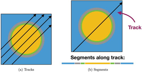
The scalar flux in each flat source region (FSR) is defined by numerically approximating the spatial and angular integral of the scalar fluxes and the volumes using the tracks crossing each FSR. It is necessary to have a sufficient number of tracks (indexed by k) crossing each FSR to ensure accurate evaluation of the scalar flux. Figure 2a shows an illustrative set of a few tracks. The intersections of a track on the boundary of each successive FSR define the segments, as shown in Fig. 2b. Using the fact that each track has an assigned spacing/width ${\omega }_k$, the scalar flux is

(5) ${\bar{\varphi }}_{i,g}=\frac{4\pi }{{\mathrm{\Sigma }}_{t,i,g}}\left[Q_{i,g}+\frac{1}{V_i}\sum _k\sum _p{\omega }_m(k){\omega }_p{\omega }_k\mathrm{\Delta }{\psi }_{k,i,g,p}\right],$(5)

Fig. 2. Example of equally spaced tracks and the segments that would lie along one such track

where

$m$ =	=	indices for azimuthal quadrature
$p$ =	=	indices for polar quadrature
$\omega$ =	=	weights.

In addition, MOCkingbird utilizes an “as-tracked” approximation of the FSR volumes, with the volumes of the FSRs approximated using track integrations.

Traditionally, segmentation is carried out as a preprocessing step by MOC-based codes,^20,52 where the tracks are traced and segments are stored in memory for later use during the iterative solution scheme. However, the number of segments required in 3D calculations can overwhelm available computer resources; therefore, recent advancements have been made in “on-the-fly” segmentation.⁹ In this mode, ray tracing is performed each time the track is used to integrate the angular flux across the domain. This provides savings in memory,⁹ but also requires additional computational work. MOCkingbird can be run in either mode: saving the segments during the first sweep or completely on-the-fly computation to save memory.

Using these approximations, it is possible to compute the scalar flux by accumulating each $\mathrm{\Delta }{\psi }_{k,i,g,p}$ computed on each segment across each FSR. Many different options exist for determining the tracks, including cyclic tracking,⁴⁰ MRT (Ref. 43), once-through,⁵³ and back-projection.³³ The track laydown algorithm used by MOCkingbird is cyclic, global tracking as developed within OpenMOC (Ref. 40).

Cyclic tracking creates track laydowns that form cycles through the domain. That is, starting at the origin of one track it is possible to move along all connected tracks in the cycle and arrive back at the starting position. Cyclic tracking is desirable for its ability to accurately represent reflected, periodic, or rotational boundary conditions. As can be seen in Fig. 3, at the edges of the domain each track meets the next track in the cycle. This allows for the angular flux to pass from one track to the next track. Without this feature, the incoming angular flux at the beginning of the tracks would have to be approximated or known. In full-core calculations, the incoming angular flux is often zero (vacuum), but having cyclic tracking capability makes the code much more flexible for the calculation of symmetric problems (e.g., pin cells and assembly-level lattice calculations).

Fig. 3. (a) Two-dimensional and (b) three-dimensional, with the 3D tracks defined as “stacks” above the 2D tracks (from Ref. 40)

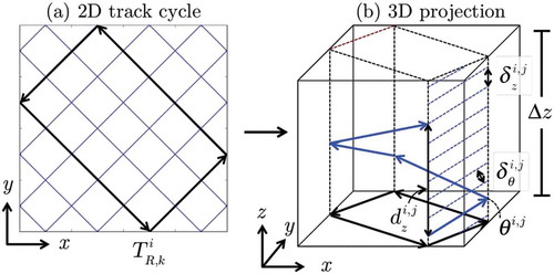
The cyclic tracking code utilized in MOCkingbird was initially developed for OpenMOC, as detailed in Ref. 40. As shown in Fig. 3, the algorithms produce 2D tracks by specifying the number of azimuthal angles and the azimuthal spacing (space between parallel tracks). For 3D tracks, the 2D tracks are generated first. Then, “stacks” are made above each 2D track to create the 3D tracks. However, just as in segmentation, the storage of all of the 3D track information can be prohibitive for a full-core 3D calculation. The index of the 2D track uniquely identifies each 3D track it projects to, the index of its polar angle, and its index in the z-stack of tracks. This allows MOCkingbird to create a 3D track on-the-fly, enabling parallelizable track generation.

MOCkingbird includes support for stochastic angular quadratures in addition to the traditional discrete ordinates angular quadrature. The Random Ray Method⁵⁴ (TRRM) integrates the angular flux across noncyclical tracks chosen randomly within the domain. The premise of a stochastic quadrature in MOC was originally exposed by Davidenko and Tsibulsky in the Russian language work⁵¹ and later recapitulated in English in Appendix B of Ref. 55, giving promising results on the C5G7 benchmark. The idea of a stochastic quadrature had not enjoyed further analysis or examination in English language works up until Tramm et al.’s recent introduction of TRRM. We have utilized Tramm et al.’s research by including TRRM mode in MOCkingbird. One significant advantage of TRRM is reduced memory usage when compared to deterministic track laydowns. This MOCkingbird capability will be discussed in a future publication.

IV.C. Source Iteration and Transport Sweeps

MOCkingbird utilizes a source iteration scheme for the angular fluxes along each track, scalar fluxes in each FSR, and the eigenvalue that balances the system. The scheme iterates between sweeping the angular fluxes across the tracks and updating the flat sources using the scalar fluxes computed during sweeping.

Algorithm 1 outlines the source iteration scheme. First, the fluxes are initialized, then the scalar fluxes are utilized to compute the initial source $Q$. The scalar and domain boundary angular fluxes are then normalized by dividing by the sum of the fission source (which is computed using an MPI_Allreduce in parallel):

(6) $F=\sum _i\sum _g\nu {\mathrm{\Sigma }}_{i,f,g}{\varphi }_{i,g}.$(6)

Normalization is necessary to keep the source values from continually increasing/decreasing (depending on the value of k_eff).

The scalar flux and FSR volumes are then zeroed for accumulation during the transport sweep. The transport sweep itself is shown in Algorithm 2. Each segment of each track is iterated over, the angular flux is updated, and the contribution to the scalar flux is tallied according to Eq. (5)(5) ${\bar{\varphi }}_{i,g}=\frac{4\pi }{{\mathrm{\Sigma }}_{t,i,g}}\left[Q_{i,g}+\frac{1}{V_i}\sum _k\sum _p{\omega }_m(k){\omega }_p{\omega }_k\mathrm{\Delta }{\psi }_{k,i,g,p}\right],$(5) . When integration across a track meets a partition boundary, the current angular flux is packed into a data structure and communicated to the neighboring process via an asynchronous MPI communication algorithm, which will be detailed in a later publication.

After the transport sweep, the eigenvalue is updated using the ratio of the old and new fission sources [as computed using Eq. (6(6) $F=\sum _i\sum _g\nu {\mathrm{\Sigma }}_{i,f,g}{\varphi }_{i,g}.$(6) ), and utilizing MPI_Allreduce in parallel]:

(7) $k_{eff,\mathrm{n}\mathrm{e}\mathrm{w}}=k_{eff,\mathrm{o}\mathrm{l}\mathrm{d}}\frac{F_{\mathrm{n}\mathrm{e}\mathrm{w}}}{F_{\mathrm{o}\mathrm{l}\mathrm{d}}},$(7)

and then convergence criteria are checked. MOCkingbird convergence criteria are based on the root-mean-squared (RMS) change of the element fission source:

(8) $F_{\mathrm{R}\mathrm{M}\mathrm{S}}=\sqrt{\frac{{{\sum }_{\mathrm{f}\mathrm{i}\mathrm{s}\mathrm{s}\mathrm{i}\mathrm{o}\mathrm{n}\mathrm{a}\mathrm{b}\mathrm{l}\mathrm{e},i}\left(\frac{\sum _g{\mathrm{\Sigma }}_{f,i,g}{\varphi }_{i,g,\mathrm{n}\mathrm{e}\mathrm{w}}-\sum _g{\mathrm{\Sigma }}_{f,i,g}{\varphi }_{i,g,\mathrm{o}\mathrm{l}\mathrm{d}}}{\sum _g{\mathrm{\Sigma }}_{f,i,g}{\varphi }_{i,g,\mathrm{o}\mathrm{l}\mathrm{d}}}\right)}^2}{N_{\mathrm{f}\mathrm{i}\mathrm{s}\mathrm{s}\mathrm{i}\mathrm{o}\mathrm{n}\mathrm{a}\mathrm{b}\mathrm{l}\mathrm{e}}}},$(8)

where fissionable refers to FSRs that contain fissionable material, and $N$ is the number of fissionable elements. The sum over fissionable elements is computed in parallel utilizing MPI_Allreduce. The change in k_eff is also monitored:

(9) $\mathrm{\Delta }k=\left|k_{eff,\mathrm{n}\mathrm{e}\mathrm{w}}-k_{eff,\mathrm{o}\mathrm{l}\mathrm{d}}\right|.$(9)

Once $F_{\mathrm{R}\mathrm{M}\mathrm{S}}$ or $\mathrm{\Delta }k$ is small enough (typically ${10}^{-4}$ and ${10}^{-6}$), the iteration is terminated. It should be noted that these conditions are sometimes referred to as “stopping criteria” rather than “convergence criteria,” as these quantities are not true residuals.

IV.D. Transport Correction and Stabilization

Transport-corrected cross sections have been shown to sometimes cause the source iteration scheme outlined previously to diverge.⁵⁶ The transport correction is a modification to the cross sections to take anisotropic effects into account.⁵⁷ Using $\mathrm{\Delta }{\mathrm{\Sigma }}_{tr,g}$ as the correction, it is applied through modification of the total and scattering cross sections:

(10) ${\mathrm{\Sigma }}_{tr,g}={\mathrm{\Sigma }}_{t,g}-\mathrm{\Delta }{\mathrm{\Sigma }}_{tr,g}$(10)

and

(11) ${\tilde{\mathrm{\Sigma }}}_{s,g{ }^{\mathrm{\prime }}\to g}={\mathrm{\Sigma }}_{s0,g{ }^{\mathrm{\prime }}\to g}-\mathrm{\Delta }{\mathrm{\Sigma }}_{tr,g}{\delta }_{g{ }^{\mathrm{\prime }},g}.$(11)

Making these cross-section modifications can lead to a system that is unstable under source iteration. For an in-depth analysis see Refs. 9 and 56. MOCkingbird stabilizes this using the damping scheme of Ref. 56. This is achieved by defining a damping factor:

(12) $D_{i,g}=\left\{\begin{array}{cc}\frac{-\rho {\tilde{\mathrm{\Sigma }}}_{s,i,g\to g}}{{\mathrm{\Sigma }}_{tr,i,g}},& \mathrm{f}\mathrm{o}\mathrm{r}{\mathrm{\Sigma }}_{s0,i,g\to g}<0\\ 0,& \mathrm{o}\mathrm{t}\mathrm{h}\mathrm{e}\mathrm{r}\mathrm{w}\mathrm{i}\mathrm{s}\mathrm{e},\end{array}\right.$(12)

where $\rho >0$ controls the amount of damping to apply for FSRs that have negative in-group scattering cross sections. Larger values of $\rho$ lead to more damping. Too much damping, though, will slow the convergence rate.⁹

The application of this damping factor occurs immediately after the transport sweep. The new scalar fluxes ${\varphi }_{i,g,\mathrm{n}\mathrm{e}\mathrm{w}}$ are combined with the scalar fluxes from the previous iteration ${\varphi }_{i,g,\mathrm{o}\mathrm{l}\mathrm{d}}$ via a weighted average:

(13) ${\varphi }_{i,g}=\frac{{\varphi }_{i,g,\mathrm{n}\mathrm{e}\mathrm{w}}+D_{i,g}{\varphi }_{i,g,\mathrm{o}\mathrm{l}\mathrm{d}}}{1+D_{i,g}}.$(13)

The new k_eff is computed using this damped flux. Damping is only applied if $\rho$ is specified to be a positive number, thus it is only used when problems require it.

IV.E. Parallelism and Domain Decomposition

The MOC is a highly parallelizable algorithm. The majority of the computational effort is located within the transport sweep, and each independent track can be swept simultaneously. This inherent parallelism is, in most scalable MOC codes, exploited by a combination of shared and distributed memory parallelism. OpenMP (Ref. 58) is the usual shared memory choice for MOC used in Refs. 9, 20, 31, 43, and 45 even though other models like pthreads⁵⁹ could be used. Distributed memory parallelism for MOC, taking place on multiple computers connected over a network, universally uses MPI (Ref. 60) as its programming model. Graphics processing units have also been used to parallelize MOC (Ref. 46), which hold their own parallelization challenges.

A natural way to use a distributed memory cluster is to split the reactor geometry among the MPI ranks. During a transport sweep, each rank is responsible for segment integration across tracks that intersect the assigned portion of the domain. The partitioning of the domain is called SDD (Ref. 61), and has been applied to reactor geometries.^9,43 Because compute work scales with partition volume and communication scales with partition surface area, Cartesian decompositions should be effective, so long as each partition volume and contained surface area is approximately equal.⁴³ This has the caveat of being inflexible in the number of compute nodes to be used. Consider the partitioning of a cube into equal volumes; only 1, 8, 27, 64, and so on partitions are compatible with this scheme assuming the partitions are also cube shaped.

Another restriction is that MRT (Ref. 43) is often employed with SDD, in which case the rays in each partition are the same and meet each other at boundaries. This allows for a simplified communication pattern with only nearest neighbors. Within each source iteration, the incoming angular flux is set, and all rays are traced from one edge of the partition boundary to the next partition boundary and finally communicated to the neighbor. The outcome of this process is that angular flux data only move across one partition during each source iteration. Without the presence of acceleration methods, information traverses the domain more slowly than following the track completely at each iteration, inhibiting convergence, as confirmed by Ref. 9.

MOCkingbird utilizes both MPI and OpenMP for its parallelization, with an arbitrary SDD using MPI and optional OpenMP threads to process the work on each spatial domain. MOCkingbird benefits from its integration in the MOOSE framework to leverage its existing partitioning algorithms. Because MOCkingbird does not utilize either Cartesian SDD nor MRT, it is not subject to partition multiplicity restrictions or degraded transport convergence without acceleration. An arbitrary partition multiplicity may be used. Moreover, because rays are traced completely through the domain on each iteration, convergence properties for highly decomposed geometries do not differ from serial computations. This property is important for simulation reproducibility across computing platforms.

IV.F. Memory

Full-core reactor 3D simulations require enormous compute resources, but lie well within the capabilities of modern high-performance computing. For the 3D pressurized water reactor core calculation in the BEAVRS benchmark,⁶² presented in Sec. V.D, there are $1.4\times {10}^9$ FSRs, $300\times {10}^6$ tracks, and 70 energy groups. The storage of the scalar fluxes and the domain boundary angular fluxes is approximately $140\times {10}^9$ double-precision floating-point numbers (1 TB of memory). Ideally, as the problem is decomposed into smaller partitions, the total memory used should be roughly constant. However, with MRT, this is not the case.

As the number of partitions grow with MRT, so does the memory usage as the angular flux is stored at the beginning and end of each track on each partition, and the total partitions’ surface increases. To compute an estimate of the total memory that would be used by MRT for the 3D BEAVRS problem, a few assumptions are made: a 360 $\times$ 360 $\times$ 460 cm domain size, 32 azimuthal angles, four polar angles, isotropic tracks, and a domain partitioning using cubic numbers of MPI ranks. Using these assumptions, the graph in Fig. 4 is produced, showing the amount of memory used to store the partition boundary angular fluxes. The growth of memory with MPI ranks with MRT could represent an issue for usability with large-scale compute jobs. However, this could be somewhat alleviated by using hybrid distributed shared memory, in which MPI ranks are used across nodes and local (on-node), non-MPI processes are created that can share on-node memory as needed (for example, for angular fluxes between partitions on the same node).

Fig. 4. Growth of angular flux storage versus scalar flux storage when using MRT. Computed using partitioning into cubes of MPI ranks (from Ref. 43)

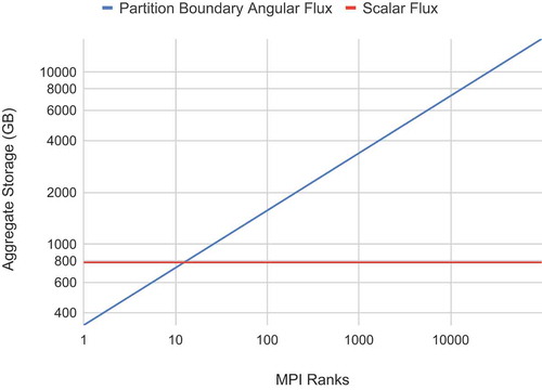
In contrast, MOCkingbird only stores angular fluxes on the global domain boundaries, as characteristics are followed across the entire domain at every sweep, so intermediate storage is not required. Therefore, there is no increase in angular flux storage as the problem is decomposed into smaller partitions. MOCkingbird still allocates a memory pool of rays and angular fluxes in each domain, but it is much smaller and only serves to avoid constant allocation and de-allocation of angular flux arrays.

V. BENCHMARK PROBLEMS

Section IV described the algorithms that MOCkingbird utilizes and their parallel performance. This section explores their efficacy for solving steady-state, k-eigenvalue, neutron transport benchmarks. Specifically, four benchmarks are analyzed: the 2D C5G7 (Ref. 55), the 3D C5G7 Rodded-B,⁶³ the 2D BEAVRS, and the 3D BEAVRS (Ref. 62).

We abbreviate the average absolute pin power error as “AVG,” the pin peaking factor–weighted average absolute pin power error as “MRE,” and the root-mean-square pin power error as “RMS.” The metric “nanoseconds per integration” (NSI) is also introduced, measuring mean segment traversal time per ray unknown, as

(14) $\mathrm{N}\mathrm{S}\mathrm{I}\equiv \frac{T}{{\sum }_k{\sum }_i{N}_g{N}_p},$(14)

where

$T$ =	=	time for a source iteration (in nanoseconds)
$k$ =	=	tracks
$i$ =	=	segments on each track
$N_g$ =	=	number of energy groups
$N_p$ =	=	number of polar angles in the polar quadrature.

When considering scalability, if the number of ranks is doubled, it would ideally be the case that the time $T$ would be cut in half, and therefore NSI would also be reduced by a factor of 2. With this, the metric “levelized nanoseconds per integration” (LNSI) is also introduced as

(15) $\mathrm{L}\mathrm{N}\mathrm{S}\mathrm{I}\equiv \frac{\mathrm{N}\mathrm{S}\mathrm{I}}{N_{\mathrm{p}\mathrm{r}\mathrm{o}\mathrm{c}\mathrm{s}}},$(15)

where $N_{\mathrm{p}\mathrm{r}\mathrm{o}\mathrm{c}\mathrm{s}}$ is the number of ranks used. This scales NSI back to a more universal metric; if a code is perfectly scaling, the LNSI stays constant. This metric has been utilized in other MOC papers.^9,20,64

V.A. 2D C5G7 Benchmark

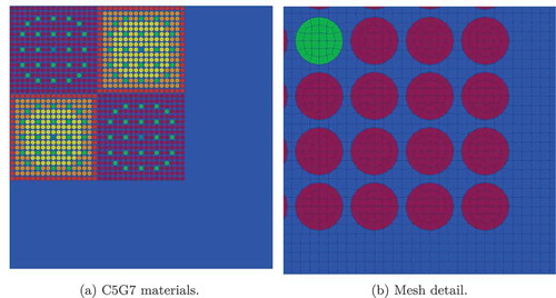
The C5G7 benchmark⁵⁵ has often been used in the literature as a verification step for deterministic transport codes.^20,21,65,66 As shown in Fig. 5, the quarter-core 2D benchmark includes four assemblies with 17 × 17 fuel pins and a water reflector. One of the defining features of the C5G7 is the heterogeneous representation of the pin cell with the exception of the clad and gap homogenization. A 112 132-element mesh, as seen in Fig. 5, was used that matches the element locations and spatial fidelity close to CSG as in Ref. 20. A quadrilateral mesh type was used. While the underlying mesh library supports higher-order elements, MOCkingbird’s ray-tracing capabilities currently only support cells with planar sides.

Fig. 5. (a) Quarter-core C5G7 geometry and (b) mesh detail for the bottom right corner of the core. Colors represent sets of fuel mixtures and the moderator

For an angular refinement study, track spacing will be held constant at 0.01 cm, while the number of azimuthal angles is increased from 4 to 128. In the polar direction, the Tabuchi Yamamoto⁶⁷ (TY) quadrature with three angles is used. $\mathrm{\Delta }\rho$ is computed against the MCNP benchmark reference k_eff of 1.18655. Convergence was judged using a fission source RMS change between successive fission source iterations of $1\times {10}^{-5}$.

The results of this study can be found in Table I. MOCkingbird converges as the number of azimuthal angles increases. These numerical results and the qualitative fluxes found in Fig. 6 agree well with other published results.²⁰ In addition, the normalized absolute relative pin power error, shown in Fig. 7, is in line with the results found in Ref. 65, showing larger error in the fuel pins near the reflector.

TABLE I The 2D C5G7 Results with Increasing Azimuthal Angles and an Azimuthal Spacing of 0.01 cm

Angles	Sweeps	keff	$\mathrm{\Delta }\rho$ (pcm)	AVG	MRE	RMS
4	648	1.18552	−102	1.95	1.78	2.42
8	656	1.18484	−169	0.43	0.38	0.53
16	656	1.18512	−139	0.27	0.20	0.38
32	655	1.18638	−14	0.28	0.22	0.40
64	654	1.18664	11	0.29	0.24	0.42
128	654	1.18676	23	0.30	0.24	0.43

Fig. 6. The 2D C5G7 results with 128 azimuthal angles and an azimuthal spacing of 0.01 cm

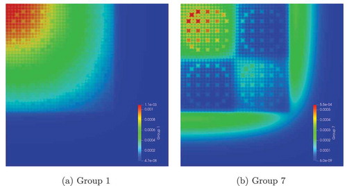
Fig. 7. The 2D C5G7 absolute relative error (in percent) in normalized pin powers with an azimuthal spacing of 0.01 cm: (a) 128 azimuthal angles and (b) 4 azimuthal angles

These simulations utilized 160 MPI ranks spread across four nodes of the Lemhi cluster at Idaho National Laboratory (INL). Table II details the performance of each run for the angular refinement study. “Solve time” is the total time to convergence in seconds spent doing source iterations. The number of iterations and intersections per iteration are also shown in Table II. The LNSI can be seen to fall and then remain constant as the number of azimuthal angles rises; this is the amortization of parallel communication latency with the addition of more work per MPI rank.

TABLE II The 2D C5G7 Performance Characteristics

Angles	Solve Time (s)	Iterations	Intersections	LNSI
4	66	648	12 014 062	41
8	77	656	22 442 732	31
16	115	656	44 105 097	25
32	194	655	88 073 264	24
64	362	654	175 991 664	24
128	770	654	351 892 634	24

V.B. 3D C5G7 Benchmark

The C5G7 benchmark has been extended to a full suite of 3D benchmarks.⁶³ There are three primary configurations in the 3D benchmark: Unrodded, Rodded A, and Rodded B, of which this study focuses on only the Rodded B because it offers the largest challenge by having multiple banks of control rods partially inserted.

Four meshes were created with 50, 100, 200, and 400 axial layers, which contain 5.6, 11.2, 22.4, and 44.8 M elements, respectively. The meshes were extruded from our C5G7 mesh, with 32 azimuthal angles with a spacing of 0.1 cm and six polar angles with 0.3 cm axial spacing chosen. This resulted in the generation of 53.9 M tracks. These simulations utilized 400 MPI ranks and ten nodes on the Lemhi cluster (two processors per node with 20 cores per processor and 192 GB memory) at INL. The convergence criteria were ${10}^{-5}$ relative change in the fission source. The results of this study can be found in Table III with a representative 3D scalar flux solution shown in Fig. 8.

TABLE III The 3D C5G7 Rodded B Results with Increasing Axial Elevations

Axial Layers	keff	$\mathrm{\Delta }\rho$ (pcm)	AVG	RMS
50	1.073129	−464	$0.892$	$1.160$
100	1.076307	−146	$0.571$	$0.825$
200	1.077239	−53	$0.492$	$0.739$
400	1.077498	−27	$0.470$	$0.713$

Fig. 8. The 3D C5G7 thermal scalar flux with 50 axial layers

With these results, it is seen that MOCkingbird achieves a k_eff within 50 pcm of the benchmark solution on the finest grid. It is clear that axial fidelity plays a large role in accuracy, as the coarsest mesh has an eigenvalue that is 464 pcm too low.

A polar angle study was also completed. The 400-axial-layer mesh was used with the same configuration noted previously, spare for the number of polar angles. The detailed results can be viewed in Table IV. While the error is already low by six polar angles, a stationary point is not met until ten polar angles.

TABLE IV The 3D C5G7 Rodded B Polar Angle Study Results

Angles	Sweeps	keff	$\mathrm{\Delta }\rho$ (pcm)	AVG	MRE	RMS
2	708	1.082	465	1.519	1.250	2.259
4	706	1.078	29	0.602	0.482	0.960
6	709	1.077	−27	0.470	0.386	0.713
8	710	1.077	−43	0.428	0.358	0.629
10	711	1.077	−49	0.408	0.344	0.587
12	711	1.078	−50	0.396	0.336	0.563

Table V details the performance of MOCkingbird for the solution of the C5G7 Rodded B. One interesting trend in Table V is that the LNSI increases as the amount of axial layers increases. All solves were performed using 400 MPI ranks; therefore, increasing the mesh density should, in theory, increase the amount of local work to be done and decrease LNSI. However, additional cache misses will occur due to the greater number of elements traversed in an unstructured manner during ray tracing.

TABLE V The 3D C5G7 Performance Characteristics

Axial Layers	Solve Time (s)	Iterations	LNSI	Intersections/Iterations
50	15 488	700	99	12 386 466 041
100	18 575	707	110	13 380 319 921
200	24 561	709	126	15 370 859 231
400	33 659	709	138	19 351 886 010

V.C. 2D BEAVRS Benchmark

The BEAVRS benchmark⁶² was developed at the Massachusetts Institute of Technology (MIT) as a realistic benchmark with real-world measurements for comparison. It is a full-core benchmark containing 193 fuel assemblies, each with an array of 17 × 17 fuel rods, guide tubes, and burnable poisons. Two fuel cycles are contained within the benchmark; however, the current study focuses on the fresh core configuration from cycle 1. This section solves a 2D configuration of the BEAVRS benchmark while Sec. V.D explores a fully 3D solution.

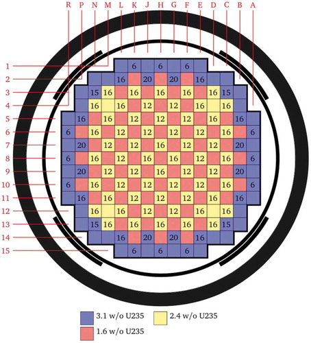
The layout of the assemblies for cycle 1 can be seen in Fig. 9. There are three different levels of enrichment: 3.1%, 2.4%, and 1.6%, and multiple layouts of burnable poisons (6, 12, and 16). Each pin cell is fully specified by the benchmark, without any homogenization.

Fig. 9. BEAVRS benchmark assembly layout for cycle 1(Ref. 62)

V.C.1. Meshing

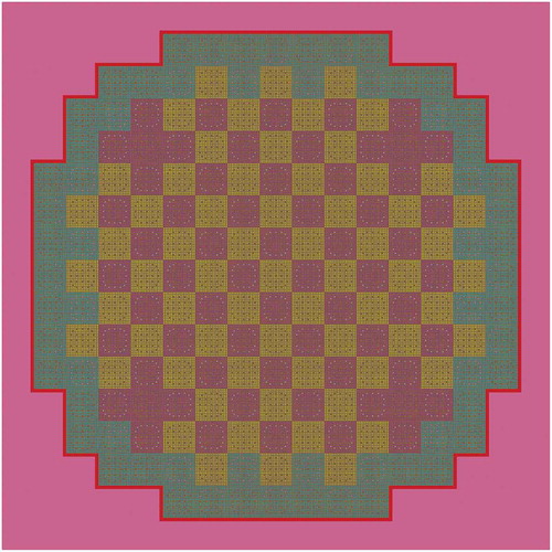
The 2D mesh is built using pin cells generated from Cubit,⁶⁸ as shown in Fig. 10, which are then utilized in the MeshGenerator system to create assemblies and ultimately the core. In addition to the fuel assemblies, the baffle and bypass water are meshed as part of “water assemblies” in Cubit, which are then rotated to fit around the core and added to the core pattern. Figure 11 shows the baffle and water meshes. A view of the full geometry can be found in Fig. 12. Ultimately, the mesh used for this study contained 10 553 408 elements.

Fig. 10. Pin cell meshes and inter-assembly gap mesh

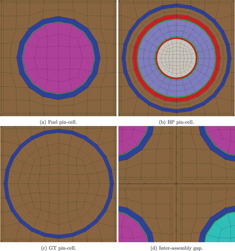
Fig. 11. Example of the baffle and water mesh surrounding the core

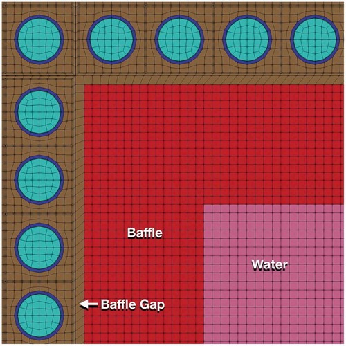
Fig. 12. As-meshed geometry for the 2D BEAVRS core

V.C.2. Cross Sections and Reference Values

The BEAVRS benchmark does not include a set of cross sections; rather, it specifies the materials in the reactor used to generate the cross sections. However, a detailed OpenMC model exists⁶⁹ that can be utilized to generate such cross sections for the Hot Zero Power isothermal case at 975 ppm boron and 560 K. For this study, Guillaume Giudicelli worked with Zhaoyuan Liu at MIT using OpenMC and the Cumulative Migration Method^57,70 to build transport-corrected 70-energy-group cross sections that are spatially averaged by material, with the reflector distinct from the moderator.

OpenMC was used to compute a normalized set of assembly powers. Those normalized powers collapsed to one of the symmetric octants of a core can be found in Fig. 13; they are used as reference values for comparison with the calculations done with MOCkingbird. Also, using this set of cross sections with OpenMOC for a detailed 2D calculation without axial leakage produced a k_eff of 1.00188 in two dimensions. That result utilized a flat source model with pin cell moderator discretized with eight rings and eight sectors and four rings and four sectors in the fuel. The OpenMOC calculation utilized 64 azimuthal angles with a 0.05-cm spacing and TY (Ref. 67) polar quadrature with three angles. The 300 pcm difference between OpenMOC and OpenMC is a resonance self-shielding error and can be resolved by introducing equivalence factors.^71–73

Fig. 13. Normalized assembly powers for the BEAVRS benchmark as computed by OpenMC . OpenMC computed eigenvalues: 2D $k_{eff}=1.00491$ and 3D $k_{eff}=1.00024$

V.C.3. Results

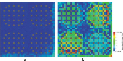
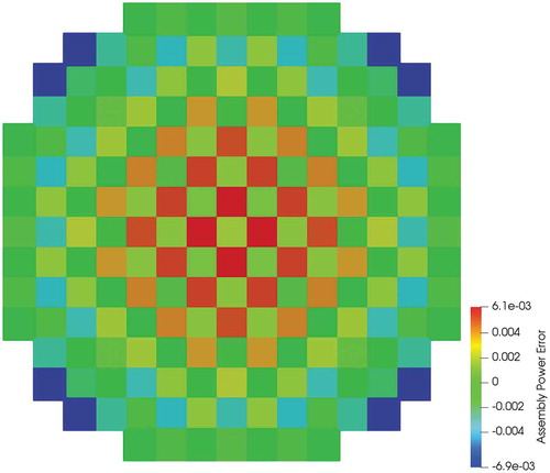
Utilizing this problem setup, MOCkingbird was run on the Lemhi cluster at the INL to solve the 2D full-core eigenvalue problem. The problem settings and computational requirements can be found in Table VI. With these settings, a k_eff of 1.00231 was computed, 43 pcm above the OpenMOC solution of Giudicelli mentioned previously. The difference can be explained by the difference between the source discretizations. In addition, as shown in Fig. 14, the normalized assembly power differences are all within 1% of the OpenMC results. The in-out tilt in the assembly power error distribution is believed to stem from shortcomings of the transport correction.^11,70

TABLE VI Problem Settings and Computational Requirements for the 2D BEAVRS

Number of elements	10 558 033
Fission source convergence	$1\times {10}^{-5}$
Azimuthal angles	64
Azimuthal spacing	0.05 cm
TY (Ref. 67) polar quadrature angles	3
MPI processes	4000
Solve time	4801 s
LNSI	19
Intersections	2 035 381 032
Number of transport sweeps	2200

Fig. 14. Normalized assembly power differences for the 2D BEAVRS solution computed by MOCkingbird compared to the OpenMC result

V.C.4. Scalability

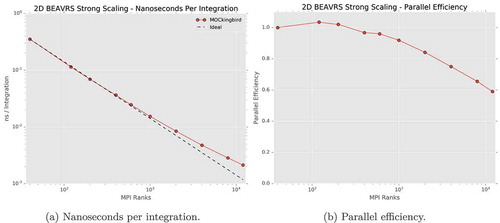
The 2D BEAVRS benchmark problem represents an ideal case to test scalability with realistic geometry and angular/spatial quadratures. A scalability study was performed with a mesh that did not represent the inter-assembly gap and therefore had 10 343 424 total elements. The results of the strong scaling study can be viewed in Fig. 16 with a representative solution shown in Fig. 15. The NSIs shown in Fig. 16a are close to ideal out to 1024 MPI processes, with performance gradually tapering off after that point. This behavior is shown in Fig. 16b, where parallel efficiency goes from over 80% at 1024 MPI processes down to 40% using 18 423 MPI processes. At 18 432 processes, each MPI rank is only responsible for 550 elements. This broad range in scalability makes MOCkingbird a flexible tool for full-core analysis.

Fig. 15. Thermal flux (0 to 9.87 ev) for the 2D BEAVRS benchmark

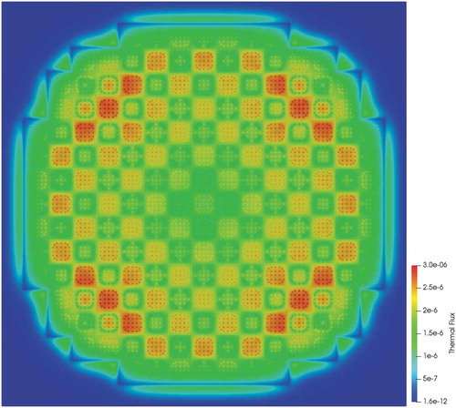
Fig. 16. Strong scaling results for 2D BEAVRS

V.D. 3D BEAVRS Benchmark

Three-dimensional simulation of the BEAVRS core is challenging due to the size of the domain and the intricate axial detail that must be modeled. In all, 34 separate axial zones must be accounted for. In addition, as shown in Refs. 9, 11, and 74 and in Sec. V.B, a fine axial discretization is needed for accuracy: optimally $<$2.0 cm mesh layers. With the core being 460 cm in height, that is more than 230 layers in the axial mesh. Due to constraints imposed by the geometrical axial elevations, 241 axial layers were required. If the full-core mesh from Sec. V.C is used as a template and extruded on 241 elevations, that is more than 2.5 billion elements.

V.D.1. Geometry and Meshing

Before running the 3D problem, the 3D mesh needs to be generated. This is accomplished using the MOOSE mesh generation capability for “extrusion.” However, due to the size and complexity of the 3D mesh for BEAVRS, this is an intricate process involving several steps. The target number of cores used for solving the 3D BEAVRS problem was chosen to be 12 000. Therefore, the mesh generation process ultimately needs to create a mesh suitable for running with that number of MPI ranks.

Within the axial elevations detailed within the BEAVRS benchmark, there are some short layers. Several are below 1 cm with the smallest being 0.394 cm. If a mesh similar to the one from Sec. V.C is extruded using those elevations, then tiny material regions, like the helium gap in a fuel pin cell, end up as tiny 3D volumes requiring a fine track laydown. To combat this, several of the small axial layers were merged, going from 34 to 26 layers. Because of similar constraints, the 40-μm assembly gaps were also neglected. A fully geometrically detailed model with angular and spatial convergence will be examined in a future report.

Generating the 3D mesh for BEAVRS used these steps:

1. Generate the 2D mesh.

2. Partition/split the 2D mesh for the number of MPI ranks to be used when running the 3D problem.

3. Using the number of MPI ranks the 3D problem will be run with, read in the split 2D mesh.

4. In parallel, extrude the mesh, changing the material definitions for each elevation.

5. Repartition the 3D mesh using the weighted hierarchical partitioner.

6. Write out the individual partitions to separate files.

Step 2 is critical because there is not enough memory for every MPI rank to read the entire 2D mesh at the same time. Therefore, each MPI process reads a small piece of it. A new parallel extrusion capability was created for step 4. Even for the 250 layers needed to create the 3D mesh, the parallel extrusion is nearly instantaneous (just seconds) due to using 12 000 MPI ranks. Without step 5, the mesh partitioning would simply be a huge number of columns (corresponding to the partitioning of the 2D mesh). Once these steps are complete, individual files, one for each MPI rank, are created that contain a portion of the 3D mesh. When MOCkingbird is ultimately run to solve the k-eigenvalue problem, each MPI rank reads its particular part of the 3D mesh.

When this process is carried out for a quarter-core 3D mesh with 241 axial layers, it generates 12 000 files containing a total of 652 854 540 elements. Those files are 162 GB in total size. To control the size of the full-core problem and make it tractable to run within the available compute time, 128 axial layers were used. This brought the 12 000 mesh files to 320 GB and 1 386 977 280 elements. That number of elements is the largest mesh ever used by a MOOSE-based application.

V.E. Three-Dimensional Core Simulations

The full-core, 3D BEAVRS problem represents an enormous challenge for any neutron transport tool. Many groups have simulated it,^75–81 some using homogenization⁸¹ and many others using Monte Carlo–based codes.^77–80 However, to date only one code^9,64 has utilized MOC for the full-core 3D analysis of BEAVRS. However, Ref. 9 also astutely made use of the extruded nature of BEAVRS to gain efficiency and reduce memory use. Also, another effort⁷⁴ solved a full-core problem similar to BEAVRS using TRRM, which differs somewhat from conventional MOC. There has yet to be a direct MOC calculation of full-core, 3D BEAVRS by a fully general, unstructured-mesh MOC code without any geometrical assumptions and the ability to perform geometric deformation. While this study is able to complete this analysis, it does so for only one mesh configuration. More work with a detailed mesh refinement study and acceleration is needed in the future.

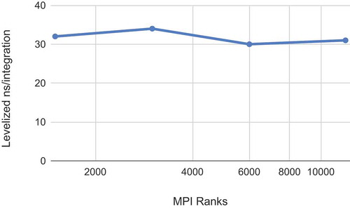
Before simulating the full-core system, a 3D quarter-core problem was used for a strong scaling study with 12 000, 6000, 3000, and 1500 MPI ranks. Figure 18 shows the results of this strong scaling study. MOCkingbird performs well, with the LNSI staying essentially constant over a large range of MPI processes. At 12 000 MPI ranks, there are, on average, over 50 000 elements per MPI rank. This suggests, based on previous scaling studies, that this problem could still scale well to around 100 000 MPI ranks. MOCkingbird’s parallel efficiency from small jobs to large makes it an efficient tool.

Fig. 17. Slices showing the detail in the top and midplane of the as-meshed full-core geometry

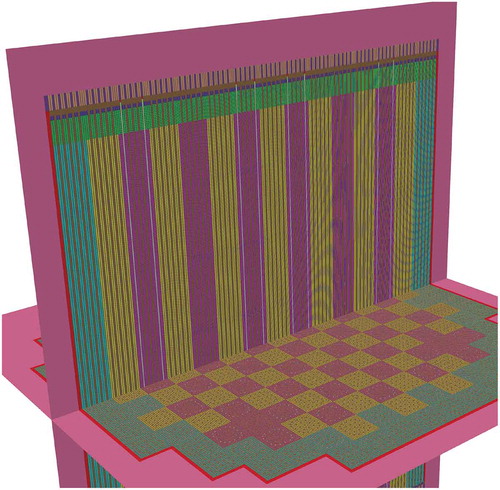
Fig. 18. Strong scaling for the 3D quarter-core BEAVRS problem. A constant LNSI equates to 100% parallel efficiency

The full-core problem represents a significant increase in computational needs. To make the problem tractable by MOCkingbird with available computational resources, the axial mesh for the full-core simulation uses 128 layers. This brings the full-core mesh, as shown in Fig. 17, to 1 386 977 280 elements. In addition, as shown in Table VII, the polar quadrature is reduced to six polar angles with a polar spacing of 2 cm. The overall effect of coarsening both spatially and angularly is that the number of tracks stays almost constant, and the number of intersections per iteration grows by less than 2×. However, solution accuracy could suffer.

TABLE VII Problem Settings and Computational Requirements for the Full-Core 3D BEAVRS Solution

Number of elements	1 386 977 280
Axial layers	128
Average element height	3.6 cm
Number of tracks	302 341 016
Fission source convergence	2E−4
keff convergence	2.1E−06
Azimuthal angles	32
Azimuthal spacing	0.1 cm
Polar angles	6
Polar spacing	2 cm
MPI processes	12 000
Solve time	33.1 h
LNSI	33
Intersections	722 139 821 713
Number of transport sweeps	800
keff	0.99402

Table

Number Of Elements	652,854,540
Axial Layers	241
Average Element Height	1.9 cm
Number of tracks	342,325,264
Fission Source Convergence	$3.6\times {10}^{-4}$
$k_{eff}$ Convergence	$5.1\times {10}^{-6}$
Azimuthal Angles	32
Azimuthal Spacing	0.1 cm
Polar Angles	8
Polar Spacing	1 cm
MPI Processes	12,000
Solve Time	(12.26 h)
LNSI	(31)
Intersections	489,712,983,737
Number of Transport Sweeps	500
$k_{eff}$	0.99381

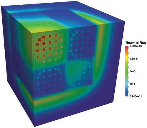
The thermal flux solution for the full-core problem is visible in Fig. 19a. The spacer grids are plain to see as thermal flux depressions. The k_eff is low at 0.99402, but that is to be expected with the coarse angular discretization and coarse axial layers. In addition to discretization error, convergence was limited (with 3× fewer power iterations than the 2D problem), and some geometric approximations were made (neglecting inter-assembly gaps and some axial homogenization of small axial zones), which both contribute to degraded solution fidelity as shown in Fig. 19b.

Fig. 19. Thermal flux for the full core shown on two slices through the core

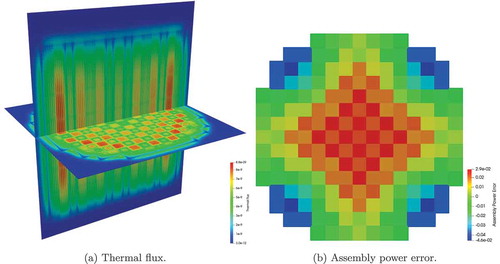
This solution, though not perfect, represents a large step forward for unstructured-mesh MOC. The result and the performance of 33 LNSI show that unstructured-mesh MOC is a viable capability for full-core reactor simulation. Once the in-progress development of an acceleration method is complete, this tool will prove to be useful for high-fidelity neutron transport calculations; at that time, this solution will be revisited.

VI. CONCLUSIONS AND FUTURE WORK

A new implementation of MOC using unstructured mesh as the underlying geometrical description, named MOCkingbird, was presented. This implementation overcomes many of the shortcomings of previous research in this area including nonvolume preserving mesh, serial track generation, approximations for boundary conditions, issues with reentrant parallel ray tracing, excessive memory usage, and load imbalances. The tool was applied to several benchmark problems to show both fidelity and scalability. Ultimately, a full-core, 3D BEAVRS benchmark calculation was achieved using 12 000 MPI ranks in 12.26 h. This result shows that the tool is capable of high-fidelity, full-core, 3D calculations. However, it should be noted that in order to enable MOCkingbird to be usable for design and analysis, a sufficient acceleration scheme needs to be developed. The next steps in this research involve completing the implementation of the acceleration method, adding transient capability, more research on mesh partitioning, generalization of the ray-tracing routines to be used by other MOOSE-based codes, and enhancements to the communication algorithms.

Acknowledgments

This work was funded under multiple programs and organizations: the INL Laboratory Directed Research and Development program and the U.S. Department of Energy (DOE) Nuclear Energy Advanced Modeling and Simulation and Consortium for Advanced Simulation of Light Water Reactors programs. This research made use of the resources of the High Performance Computing Center at INL, which is supported by the DOE Office of Nuclear Energy and the Nuclear Science User Facilities. This manuscript has been authored by Battelle Energy Alliance, LLC under contract number DE-AC07-05ID14517 with the COE. The U.S. government retains and the publisher, by accepting this article for publication, acknowledges that the U.S. government retains a nonexclusive, paid-up, irrevocable, worldwide license to publish or reproduce the published form of this manuscript, or allow others to do so, for U.S. government purposes.

References

- T. DOWNAR et al., PARCS V3. 0 US NRC Core Neutronic Simulator USER MANUAL, University of Michigan (2012).
- T. BAHADIR and S.-Ö. LINDAHL, “Studsvik’s Next Generation Nodal Code SIMULATE-5,” Proc. ANFM-2009 Conf. Advances in Nuclear Fuel Management IV, Hilton Head Island, South Carolina, April 12–15, 2009.
- M. B. IWAMOTO and M. TAMITANI, “Methods, Benchmarking, and Applications of the BWR Core Simulator Code AETNA,” Proc. Int. Conf. Advances in Nuclear Fuel Management III, Hilton Head Island, South Carolina, October 5–7, 2003.
- K. SMITH, “CASMO-4 Characteristics Methods for Two-Dimensional PWR and BWR Core Calculations,” Trans. Am. Nucl. Soc., 83, 322 (2000).
- R. SANCHEZ et al., “APOLLO II: A User-Oriented, Portable, Modular Code for Multigroup Transport Assembly Calculations,” Nucl. Sci. Eng., 100, 3, 352 (1988); https://doi.org/10.13182/NSE88-3.
- J. CASAL, “HELIOS: Geometric Capabilities of a New Fuel-Assembly Program,” Proc. Int. Topl. Mtg. Advances in Mathematics, Computations and Reactor Physics, Pittsburgh, Pennsylvania, April 28–May 2, 1991, Vol. 2, 10.2.1 1 (1991); https://ci.nii.ac.jp/naid/10016744853/en/ ( current as of July 30, 2020).
- D. KNOTT and E. WEHLAGE, “Description of the LANCER02 Lattice Physics Code for Single-Assembly and Multibundle Analysis,” Nucl. Sci. Eng., 155, 3, 331 (2007); https://doi.org/10.13182/NSE155-331.
- B. FONTAINE et al., “Description and Preliminary Results of PHENIX Core Flowering Test,” Nucl. Eng. Des., 241, 10, 4143 (2011); https://doi.org/10.1016/j.nucengdes.2011.08.041.
- G. GUNOW, “Full Core 3D Neutron Transport Simulation Using the Method of Characteristics with Linear Sources,” PhD Thesis, Department of Nuclear Science and Engineering, Massachusetts Institute of Technology (2018).
- G. GUNOW, B. FORGET, and K. SMITH, “Full Core 3D Simulation of the BEAVRS Benchmark with OpenMOC,” Ann. Nucl. Energy, 134, 299 (2019); https://doi.org/10.1016/j.anucene.2019.05.050.
- G. GIUDICELLI, “A Novel Equivalence Method for High Fidelity Hybrid Stochastic-Deterministic Neutron Transport Simulations,” PhD Thesis, Department of Nuclear Science and Engineering, Massachusetts Institute of Technology (2020).
- S. SANTANDREA, L. GRAZIANO, and D. SCIANNANDRONE, “Accelerated Polynomial Axial Expansions for Full 3D Neutron Transport MOC in the APOLLO3 Code System as Applied to the ASTRID Fast Breeder Reactor,” Ann. Nucl. Energy, 113, 194 (2018); https://doi.org/10.1016/j.anucene.2017.11.010.
- B. LINDLEY et al., “Developments Within the WIMS Reactor Physics Code for Whole Core Calculations,” presented at the Int. Conf. on Mathematics & Computational Methods Applied to Nuclear Science & Engineering, Jeju, Korea, April 16–20, 2017.
- P. ARCHIER et al., “Validation of the Newly Implemented 3D TDT-MOC Solver of APOLLO3 Code on a Whole 3D SFR Heterogeneous Assembly,” presented at PHYSOR, Sun Valley, Idaho, May 1–5, 2016.
- J. R. TRAMM et al., “ARRC: A Random Ray Neutron Transport Code for Nuclear Reactor Simulation,” Ann. Nucl. Energy, 112, 693 (2018); https://doi.org/10.1016/j.anucene.2017.10.015.
- D. GASTON et al., “MOOSE: A Parallel Computational Framework for Coupled Systems of Nonlinear Equations,” Nucl. Eng. Des., 239, 10, 1768 (2009); https://doi.org/10.1016/j.nucengdes.2009.05.021.
- C. J. PERMANN et al., “MOOSE: Enabling Massively Parallel Multiphysics Simulation,” SoftwareX, 11, 100430 (2020); https://doi.org/10.1016/j.softx.2020.100430.
- J. ASKEW, “A Characteristics Formulation of the Neutron Transport Equation in Complicated Geometries,” United Kingdom Atomic Energy Authority (1972).
- D. KNOTT and A. YAMAMOTO, “Lattice Physics Computations,” Handbook of Nuclear Engineering, pp. 913–1239, D. G. CACUCI, Ed., Springer (2010); https://doi.org/10.1007/978-0-387-98149-9.
- W. BOYD et al., “The OpenMOC Method of Characteristics Neutral Particle Transport Code,” Ann. Nucl. Energy, 68, 43 (2014); https://doi.org/10.1016/j.anucene.2013.12.012.
- B. KOCHUNAS et al., “Overview of Development and Design of MPACT: Michigan Parallel Characteristics Transport Code,” Proc. 2013 Int. Conf. Mathematics and Computational Methods Applied to Nuclear Science and Engineering (M and C 2013), Sun Valley, Idaho, May 5–9, 2013.
- K. S. SMITH, “Nodal Method Storage Reduction by Nonlinear Iteration,” Trans. Am. Nucl. Soc., 44, 265 (1983).
- R. E. ALCOUFFE, “Diffusion Synthetic Acceleration Methods for the Diamond-Differenced Discrete-Ordinates Equations,” Nucl. Sci. Eng., 64, 2, 344 (1977); https://doi.org/10.13182/NSE77-1.
- C. RABITI et al., “Parallel Method of Characteristics on Unstructured Meshes for the UNIC Code,” Proc. Int. Conf. Physics of Reactors, Interlaken, Switzerland, September 14–19, 2008.
- K. S. SMITH and J. D. RHODES, “Full-Core, 2-D, LWR Core Calculations with CASMO-4E,” presented at PHYSOR 2002, Seoul, Korea, October 7–10, 2002.
- T. M. EVANS et al., “Denovo: A New Three-Dimensional Parallel Discrete Ordinates Code in SCALE,” Nucl. Technol., 171, 2, 171 (2010); https://doi.org/10.13182/NT171-171.
- A. ZHU et al., “Transient Methods for Pin-Resolved Whole Core Transport Using the 2D-1D Methodology in MPACT,” Proc. M&C 2015, Nashville, Tennessee, April 19–23, 2015, p. 19 (2015).
- M. W. REED, “The “Virtual Density” Theory of Neutronics,” Thesis, PhD Thesis, Department of Nuclear Science and Engineering, Massachusetts Institute of Technology (2014); https://dspace.mit.edu/handle/1721.1/87497 (current as of July 30, 2020).
- Y. WANG, “Nonlinear Diffusion Acceleration for the Multigroup Transport Equation Discretized with S N and Continuous FEM with Rattlesnake,” Proc. 2013 Int. Conf. Mathematics and Computational Methods Applied to Nuclear Science Engineering (M and C 2013), Sun Valley, Idaho, May 5–9, 2013.
- M. L. ADAMS and E. W. LARSEN, “Fast Iterative Methods for Discrete-Ordinates Particle Transport Calculations,” Prog. Nucl. Energy, 40, 1, 3 (2002); https://doi.org/10.1016/S0149-1970(01)00023-3.
- S. SANTANDREA et al., “A Neutron Transport Characteristics Method for 3D Axially Extruded Geometries Coupled with a Fine Group Self-Shielding Environment,” Nucl. Sci. Eng., 186, 3, 239 (2017); https://doi.org/10.1080/00295639.2016.1273634.
- A. MARIN-LAFLECHE, M. SMITH, and C. LEE, “Proteus-MOC: A 3D Deterministic Solver Incorporating 2D Method of Characteristics,” Proc. 2013 Int. Conf. Mathematics and Computational Methods Applied to Nuclear Science Engineering (M and C 2013), Sun Valley, Idaho, May 5–9, 2013.
- M. SMITH et al., “Method of Characteristics Development Targeting the High Performance Blue Gene/P Computer at Argonne National Laboratory,” Int. Conf. Mathematics and Computational Methods Applied to Nuclear Science Engineering (M&C 2011), Rio de Janeiro, Brazil, May 8–12, 2011.
- N. CHO, G. LEE, and C. PARK, “Fusion Method of Characteristics and Nodal Method for 3D Whole Core Transport Calculation,” Trans. Am. Nucl. Soc., 86, 322 (2002).
- B. COLLINS et al., “Stability and Accuracy of 3D Neutron Transport Simulations Using the 2D/1D Method in MPACT,” J. Comput. Phys., 326, 612 (2016); https://doi.org/10.1016/j.jcp.2016.08.022.
- C. LEE et al., “Simulation of TREAT Cores Using High-Fidelity Neutronics Code PROTEUS,” Proc. M&C 2017, Jeju, Korea, April 16–20, 2017, p. 16 (2017).
- X. YANG and N. SATVAT, “MOCUM: A Two-Dimensional Method of Characteristics Code Based on Constructive Solid Geometry and Unstructured Meshing for General Geometries,” Ann. Nucl. Energy, 46, 20 (2012); https://doi.org/10.1016/j.anucene.2012.03.009.
- P. COSGROVE and E. SHWAGERAUS, “Development of MoCha-Foam: A New Method of Characteristics Neutron Transport Solver for OpenFOAM,” presented at the Int. Conf. Mathematics & Computational Methods Applied to Nuclear Science Engineering (M&C 2017), Jeju, Korea, April 16–20, 2017.
- T. MAZUMDAR and S. DEGWEKER, “Solution of the Neutron Transport Equation by the Method of Characteristics Using a Linear Representation of the Source Within a Mesh,” Ann. Nucl. Energy, 108, 132 (2017); https://doi.org/10.1016/j.anucene.2017.04.011.
- S. SHANER et al., “Theoretical Analysis of Track Generation in 3D Method of Characteristics,” presented at the Joint Int. Conf. Mathematics and Computation (M&C), Nashville, Tennessee, April 19–23, 2015.
- M. FORUM, “MPI: A Message-Passing Interface Standard. Version 3.0” (2015): https://www.mpi-forum.org/docs/mpi-3.1/mpi31-report.pdf (accessed Aug. 23, 2019).
- W. WU et al., “Improvements of the CMFD Acceleration Capability of OpenMOC,” Nucl. Eng. Technol., 52, 10, 2162 (2020); https://doi.org/10.1016/j.net.2020.04.001.
- B. M. KOCHUNAS, “A Hybrid Parallel Algorithm for the 3-D Method of Characteristics Solution of the Boltzmann Transport Equation on High Performance Compute Clusters.” PhD Thesis, Nuclear Engineering and Radiological Sciences, University of Michigan (2013).
- G. COLOMER et al., “Parallel Algorithms for Sn Transport Sweeps on Unstructured Meshes,” J. Comput. Phys., 232, 1, 118 (2013); https://doi.org/10.1016/j.jcp.2012.07.009.
- J. I. VERMAAK et al., “Massively Parallel Transport Sweeps on Meshes with Cyclic Dependencies,” J. Comput. Phys., 425, 109892 (2021); https://doi.org/10.1016/j.jcp.2020.109892.
- W. BOYD, “Reactor Agnostic Multi-Group Cross Section Generation for Fine-Mesh Deterministic Neutron Transport Simulations,” PhD Thesis, Department of Nuclear Science and Engineering, Massachusetts Institute of Technology (2017).
- G. I. BELL and S. GLASSTONE, “Nuclear Reactor Theory,” U.S. Atomic Energy Commission, Washington, District of Columbia (1970).
- A. HÉBERT, Applied Reactor Physics, 2nd ed., Presses Internationales Polytechnique (2009).
- S. STIMPSON, B. COLLINS, and B. KOCHUNAS, “Improvement of Transport-Corrected Scattering Stability and Performance Using a Jacobi Inscatter Algorithm for 2D-MOC,” Ann. Nucl. Energy, 105, 1 (2017); https://doi.org/10.1016/j.anucene.2017.02.024.
- V. VLADIMIROV, “Numerical Solution of the Kinetic Equation for the Sphere,” Vycisl. Mat., 3, 3 (1958).
- V. DAVIDENKO and V. TSIBULSKY, “The Method of Characteristics with Angle Directions Stochastic Choice,” Math. Mod., 15, 8, 75 (2003); http://www.mathnet.ru/php/archive.phtml?wshow=paper&jrnid=mm&paperid=411&option_lang=rus (accessed July 14, 2020).
- J. RHODES, K. SMITH, and D. LEE, “CASMO-5 Development and Applications,” Proc. Int. Conf. Physics of Reactors (PHYSOR2006), Vancouver, Canada, September 10–14, 2006.
- B. LINDLEY et al., “Developments Within the WIMS Reactor Physics Code for Whole Core Calculations,” Proc. M&C, Jeju, Korea, April 16–20, 2017.
- J. R. TRAMM et al., “The Random Ray Method for Neutral Particle Transport,” J. Comput. Phys., 342, 229 (2017); https://doi.org/10.1016/j.jcp.2017.04.038.
- E. LEWIS et al., “Benchmark Specification for Deterministic 2-D/3-D MOX Fuel Assembly Transport Calculations without Spatial Homogenization (C5G7 MOX), Nuclear Energy Agency / Nuclear Science Committee (2001).
- G. GUNOW, B. FORGET, and K. SMITH, “Stabilization of Multi-Group Neutron Transport with Transport-Corrected Cross-sections,” Ann. Nucl. Energy, 126, 211 (2019); https://doi.org/10.1016/j.anucene.2018.10.036.
- Z. LIU et al., “Cumulative Migration Method for Computing Rigorous Diffusion Coefficients and Transport Cross Sections from Monte Carlo,” Ann. Nucl. Energy, 112, 507 (2018); https://doi.org/10.1016/j.anucene.2017.10.039.
- L. DAGUM and R. MENON, “OpenMP: An Industry Standard API for Shared-Memory Programming,” IEEE Comput. Sci. Eng., 5, 1, 46 (1998); https://doi.org/10.1109/99.660313.
- B. NICHOLS, D. BUTTLAR, and J. FARRELL, PThreads Programming: A POSIX Standard for Better Multiprocessing, O’Reilly Media, Inc. (1996).
- W. GROPP et al., “A High-Performance, Portable Implementation of the MPI Message Passing Interface Standard,” Parallel Comput., 22, 6, 789 (1996); https://doi.org/10.1016/0167-8191(96)00024-5.
- B. KELLEY et al., “CMFD Acceleration of Spatial Domain-Decomposition Neutron Transport Problems,” Proc. Int. Conf. Physics of Reactors (PHYSOR2012), Knoxville, Tennessee, April 15–20, 2012.
- N. HORELIK et al., “Benchmark for Evaluation and Validation of Reactor Simulations (BEAVRS), V1. 0.1,” Proc. Int. Conf. Mathematics and Computational Methods Applied to Nuclear Science & Engineering, Sun Valley, Idaho, May 5–9, 2013.
- “Benchmark on Deterministic Transport Calculations Without Spatial Homogenisation, MOX Fuel Assembly 3D Extension Case,” Organisation for Economic Co-operation and Development/Nuclear Energy Agency (2005).
- G. GIUDICELLI et al., “Adding a Third Level of Parallelism to OpenMOC, an Open Source Deterministic Neutron Transport Solver,” presented at the Int. Conf. Mathematics and Computational Methods Applied to Nuclear Science and Engineering, Portland, Oregon, August 25–29, 2019.
- R. M. FERRER and J. D. RHODES III, “A Linear Source Approximation Scheme for the Method of Characteristics,” Nucl. Sci. Eng., 182, 2, 151 (2016); https://doi.org/10.13182/NSE15-6.
- X. YANG, R. BORSE, and N. SATVAT, “{MOCUM} Solutions and Sensitivity Study for {C5G7} Benchmark,” Ann. Nucl. Energy, 96, 242 (2016); https://doi.org/10.1016/j.anucene.2016.05.030.
- A. YAMAMOTO et al., “Derivation of Optimum Polar Angle Quadrature Set for the Method of Characteristics Based on Approximation Error for the Bickley Function,” J. Nucl. Sci. Technol., 44, 2, 129 (2007); https://doi.org/10.1080/18811248.2007.9711266.
- T. D. BLACKER, W. J. BOHNHOFF, and T. L. EDWARDS, “CUBIT Mesh Generation Environment. Volume 1: Users Manual,” Sandia National Labs (1994).
- “PWR Benchmarks” (2019); https://github.com/mit-crpg/PWR_benchmarks ( current as of July 30, 2020).
- Z. LIU et al., “Conservation of Migration Area by Transport Cross Sections Using Cumulative Migration Method in Deterministic Heterogeneous Reactor Transport Analysis,” Prog. Nucl. Energy, 127, 103447 (2020); https://doi.org/10.1016/j.pnucene.2020.103447.
- G. GIUDICELLI, K. SMITH, and B. FORGET, “Generalized Equivalence Methods for 3D Multi-Group Neutron Transport,” Ann. Nucl. Energy, 112, 9 (2018); https://doi.org/10.1016/j.anucene.2017.09.024.
- H. PARK and H. G. JOO, “Practical Resolution of Angle Dependency of Multigroup Resonance Cross Sections Using Parametrized Spectral Superhomogenization Factors,” Nucl. Eng. Technol., 49, 6, 1287 (2017); https://doi.org/10.1016/j.net.2017.07.015.
- G. GIUDICELLI, K. SMITH, and B. FORGET, “Generalized Equivalence Theory Used with Spatially Linear Sources in the Method of Characteristics for Neutron Transport,” Nucl. Sci. Eng., 194, 1044 (2020); https://doi.org/10.1080/00295639.2020.1765606.
- J. TRAMM, “Development of the Random Ray Method of Neutral Particle Transport for High-Fidelity Nuclear Reactor Simulation,” PhD Thesis, Department of Nuclear Science and Engineering, Massachusetts Institute of Technology (2018).
- J. LEPPÄNEN, R. MATTILA, and M. PUSA, “Validation of the Serpent-ARES Code Sequence Using the MIT BEAVRS benchmark—Initial Core at HZP Conditions,” Ann. Nucl. Energy, 69, 212 (2014); https://doi.org/10.1016/j.anucene.2014.02.014.
- M. RYU et al., “Solution of the BEAVRS Benchmark Using the nTRACER Direct Whole Core Calculation Code,” J. Nucl. Sci. Technol., 52, 7–8, 961 (2015); https://doi.org/10.1080/00223131.2015.1038664.
- D. J. KELLY et al., “Analysis of Select BEAVRS PWR Benchmark Cycle 1 Results Using MC21 and OpenMC,” Proc. Int. Conf. Physics of Reactors (PHYSOR2014), Kyoto, Japan, September 28–October 3, 2014.
- H. J. PARK et al., “Real Variance Analysis of Monte Carlo Eigenvalue Calculation by McCARD for BEAVRS Benchmark,” Ann. Nucl. Energy, 90, 205 (2016); https://doi.org/10.1016/j.anucene.2015.12.009.
- K. WANG et al., “Analysis of BEAVRS Two-Cycle Benchmark Using RMC Based on Full Core Detailed Model,” Prog. Nucl. Energy, 98, 301 (2017); https://doi.org/10.1016/j.pnucene.2017.04.009.
- Z. WANG et al., “Validation of SuperMC with BEAVRS Benchmark at Hot Zero Power Condition,” Ann. Nucl. Energy, 111, 709 (2018); https://doi.org/10.1016/j.anucene.2017.09.045.
- M. ELLIS et al., “Initial Rattlesnake Calculations of the Hot Zero Power BEAVRS,” Idaho National Laboratory (2014).