Assessing the Structure-Based Turbulence Model Performance for Thermal Striping Applications Using Symmetric Jet Experiments

Abstract

Turbulent mixing of coolant streams can result in an oscillatory mixing phenomenon called thermal striping. These fluctuations have the potential to lead to anticipated thermal fatigue failures in advanced nuclear reactors. To predict thermal striping, robust and computationally affordable modeling tools that are capable of accurately representing complex turbulence are needed. Hybrid turbulence approaches, such as detached-eddy simulation and scale-adaptive simulation, have shown some success in resolving complex unsteady turbulence for massively separated flows, however the applicability of these models to internal flows is limited.

A STRUCTure-based (STRUCT) second-generation Unsteady Reynolds-Averaged Navier–Stokes turbulence model was recently proposed at the Massachusetts Institute of Technology to robustly extend the applicability of hybrid closures. In this work, the STRUCT model is evaluated using experimental data taken at the Reactor Cavity Cooling System separate-effects test facility at the University of Michigan. The experiments observed the interaction of parallel symmetric rectangular jets, and include measurements for mean profiles of velocity and Reynolds stresses. In the present work, the simulation results are assessed against mean profiles of velocity and Reynolds stresses, demonstrating the ability to reproduce the unsteadiness of the jets in close agreement with the measurements at considerably reduced computational cost.

Keywords:

• Computational fluid dynamics
• turbulence modeling
• jet interactions
• thermal striping

I. INTRODUCTION

Oscillatory mixing of liquid coolant streams can be a potential cause of thermal fatigue in advanced nuclear reactors. This oscillatory mixing phenomenon, called thermal striping, results in temperature fluctuations that can lead to high-cycle thermal fatigue. Cracking due to thermal striping has been observed in components of operating liquid-metal reactors, including the secondary sodium pump vessel in Phenix,^[1] a T-junction in Superphenix (SPX),^[1] a control rod guide tube in the Prototype Fast Reactor (PFR),^[2] and the primary cold trap in the BN 600 reactor.^[3] High-cycle thermal fatigue has also been observed in light water reactors; a leakage incident occurred, for example, in the reactor heat removal system of the French Civaux power plant due to a crack found on the elbow of a high- and low-temperature fluid mixing region.^[4] The cause of this crack was later identified to be high-cycle thermal fatigue.^[5]

Modeling tools are necessary to predict and characterize thermal striping in advanced reactors to prevent such failures. Because this phenomenon is fully three-dimensional and has been shown to be strongly nonlinear and highly sensitive to flow geometry, lumped parameter approaches have intrinsically limited predictive capability for thermal striping applications.^[6,7] Computational fluid dynamics (CFD) can offer necessary three-dimensional resolution and sensitivity to the geometry and turbulence details.

To capture thermal striping in CFD, turbulence must be accurately represented with robust and computationally affordable modeling tools. Although large-eddy simulations (LES) have the capability to provide reliable results by resolving most of the turbulence scales, it is still too computationally expensive to be used as an engineering tool for industrial applications. Less computationally expensive approaches include using hybrid turbulence models, such as Detached-Eddy Simulation (DES) and Scale Adaptive Simulation (SAS)^[8] and scale-adaptive simulations,^[9] have shown some successes in applications involving large flow separation. However, results from an international blind benchmark exercise for thermal striping^[10] have shown that these models fail in representing the correct unsteadiness in internal flow cases, even underperforming standard Reynolds-averaged approaches.

Recently, a second-generation hybrid turbulence model, introduced by Lenci^[11] and Lenci et al.^[12] and later reformulated by Xu,^[13,14] has been proposed to extend the hybrid concept applicability to a larger variety of cases by locally resolving unsteady flow structures. The reformulated version of this model, called STRUCT-ε, has demonstrated accuracy comparable to LES on mesh resolutions typical of Unsteady Reynolds-Averaged Navier–Stokes (URANS) methods.^[14,15] Additionally, spectral analysis in a T-junction case has shown frequency predictions consistent with large turbulent eddies.^[15]

The present work aims to extend the assessment of the STRUCT-ε turbulence model leveraging new high-fidelity experimental data from the Reactor Cavity Cooling System (RCCS) separate-effects test facility at the University of Michigan. Experimental runs at this facility consisted of interactions of 2, 4, and 6 parallel jets. Data sets from these experiments include time-averaged profiles of velocity and Reynolds stresses. The simulations demonstrated the ability of the model to accurately reproduce both velocities and Reynolds stress distributions even on coarse grids, confirming the robust applicability of the STRUCT-ε methodology. Due to the adiabatic nature of the experiments, this work has focused its attention on evaluating the ability of STRUCT-ε to accurately represent turbulence without the additional complexity of heat flux and temperature predictions, and its ability to reproduce the correct oscillation frequencies, which drive the thermal-driven fatigue accumulation. Future work will present the assessment of the frequency performance of the model on thermal oscillation predictions by leveraging new diabatic high-fidelity LES of this same RCCS facility.^[16]

II. BACKGROUND

II.A. Description of the RCCS Test Facility

Experiments used in this study were conducted in the RCCS separate-effects test facility at the University of Michigan. The test facility consists of six symmetric parallel rectangular jets intruding into an upper plenum. The working fluid is water. Experimental runs were conducted with 2, 4, and 6 jets and varying Reynolds numbers. Jet interactions were studied under isothermal conditions. The upper plenum has dimensions of 470.6 × 249.3 × 463 mm and has two circular exhaust pipes. Each jet has a width of 12.70 mm (L₁) and a length of 63.50 mm. The jets are spaced apart by 12.70 mm (S/L₁ = 1).

This facility is a scaled-down version of the RCCS Natural Convection Shutdown Heat Removal Test Facility prototype.^[17] In the prototype, the RCCS risers protrude a certain distance into the upper plenum, and this feature was replicated in the scaled-down version at the University of Michigan. However, the protrusion creates additional volumes that affect fluid entrainment by upward jets. To study the effect of protrusion depth in the scaled-down facility, the bottom wall position can be adjusted by inserting a plate. This simulation work aims to study jet interaction in geometry without protrusion. Therefore, a plate was installed to ensure the bottom wall was flush with the jet inlet (y = 63.5 mm), resulting in a modified flow domain with dimensions of 470.6 × 249.3 × 398.5 mm. An image of the test section is shown in Fig. 1. The facility is described in detail by Nunez et al.^[18] and Nunez.^[19] Mean measurements, including velocity and Reynolds stresses, were taken on a vertical plane centered over the inlet jets.

Fig. 1. Image of the RCCS test facility reproduced from Nunez.^[19]

II.B. STRUCT-ε Turbulence Model

The STRUCT is a second-generation URANS model first introduced by Lenci^[11] and Lenci et al.^[12] This approach tracks turbulent structures by comparing timescales associated with resolved and modeled turbulence. The model is activated in regions of significant scale overlap. STRUCT was reformulated by Xu^[13,14] to be implicitly dependent on the modeled timescale by introducing a source term in the turbulent dissipation transport equation of the standard k-ε model. This reformulation is called STRUCT-ε. The modified turbulent dissipation transport equation is

(1) $\begin{array}{rl}& \frac{\mathrm{\partial }\mathit{\epsilon }}{\mathrm{\partial t}}+\overline{u_j}\frac{\mathrm{\partial \epsilon }}{\mathrm{\partial t}}=\frac{\mathrm{\partial }}{\mathrm{\partial }{x}_j}\left[\left(\mathit{\nu }+\frac{{\nu }_{\tau }}{{\sigma }_k}\right)\frac{\mathrm{\partial \epsilon }}{\mathrm{\partial }{x}_j}\right]+C_{\mathit{\epsilon }1}\frac{\epsilon }{k}{P}_k-C_{\mathit{\epsilon }2}\frac{{\epsilon }^2}{\mathit{k}}\\ & +C_{\mathit{\epsilon }3}\mathit{k}\left|\bar{\mathrm{\Pi }}\right|,& (1)\end{array}$(1)

where the last term, $C_{\mathit{\epsilon }3}\mathit{k}\left|\bar{\mathrm{\Pi }}\right|$, is a source term introduced to the turbulent dissipation transport equation by the STRUCT-ε model.

As the turbulent dissipation rate is increased by the source term, the turbulent viscosity is reduced in areas of scale overlap, and turbulence is resolved instead of modeled. Reducing turbulent viscosity has been shown to provide resolution of turbulence consistently in Reynolds-averaged Navier-Stokes (RANS) simulations.^[20] The local activation of the model is the key to the general applicability of the approach. Other hybrid methodologies, being based on some form of mesh-to-model length-scale comparisons, or other not fully consistent length-scale concepts, lead to strong spurious activation of turbulence resolution, which greatly deteriorates the solution accuracy, driving strong failures, as shown in the Organisation for Economic Co-operation and Development/Nuclear Energy Agency international blind T-junction benchmark.^[10]

III. METHODOLOGY

III.A. Test Geometry and Flow Conditions

This present work focuses on a specific test configuration with four jets performed at the RCCS test facility. These flow conditions are given in Table I. The flow is under constant-density conditions; the fluid properties are given in Table II.

TABLE I Flow Conditions

Reynolds Number	Temperature (°C)	Number of Jets
13 862	23	4

TABLE II Fluid Properties: Constant Properties of Water at 1 Bar and 23°C Were Used

Property	Value
Density	997.54 kg/m^3
Dynamic viscosity	9.3216 × 10^−4 Pa⋅s

The computational fluid domain modeled in this study consists of the upper plenum, six shortened riser jets, and two shortened exhaust pipes. The inlet conditions in the model are imposed as fully developed flow and turbulence profiles obtained by separate precursory computations. Resulting velocity components and turbulent quantities (k and ε) were mapped to the inlet surface. The outlets are constant pressure boundaries. The walls are represented with standard no-slip conditions.

Simulations were created in STAR-CCM+ version 16.04.012-R8. Second-order time discretization based on the three-time-level backward Euler method and a nonoscillatory second-order upwind-based spatial interpolation with Venkatakrishna gradient limiting were used. Simulations were run with 80s of initialization followed by 240-s averaging.

III.B. Mesh Sensitivity Study

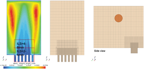
The mesh structure was based on the integral length scales (ILSs) in the measurement region of the test geometry. The ILSs were computed from a precursory RANS simulation. There are two refinement regions where the mesh is halved at each refinement: one over the jets where the ILSs are approximately 2 to 4 mm and above the jets where the ILSs are approximately 4 to 8 mm, as shown in Fig. 2. The meshing procedure aims to provide simple implementation of best practices for reactor applications, where precursory RANS simulations can be used to identify the necessary meshing requirements, thereby reducing the need for costly mesh sensitivity studies in large geometrical configurations.

Fig. 2. Mesh refinements based on ILSs.

A mesh sensitivity study was conducted for four mesh refinements, while adopting time steps that consistently produced Courant–Friedrichs–Lewy number (CFL) = 1 in the smallest refinement region. Based on grid size and CFL-driven time-step values, a representative speedup factor from LES can be calculated based on the ratio of computational cells, where LES with a modeled near wall are assumed, as resolving the wall region adds considerable additional cost. Mesh parameters and speedup factors are given in Table III.

TABLE III Mesh Parameters*

	Base Size	Refinement Zone Size/ILS	Number of Cells	Representative Speedup from LES
Mesh 1	3.00 mm	1/3	4 300 000	16×
Mesh 2	4.00 mm	1/2.3	1 840 000	50×
Mesh 3	5.33 mm	1/1.7	795 000	156×
Mesh 4	6.93 mm	1/1.3	370 000	456×

*Refinement 1 above the jets is 50% of the base size and refinement 2 overlapping the jets is 25% of the base size. Note that the refinement zone–to-ILS ratio is consistent for both refinement regions.

The mesh sensitivity was assessed with mean data sets of streamwise velocity and Reynolds stresses taken at eight evenly spaced locations on the vertical x-y plane centered over the riser jets. The x- and y-positions were normalized using the jet width L₁. The results are shown in Fig. 3.

Fig. 3. Mesh sensitivity results from top left clockwise: streamwise velocity components $\overline{u^{\prime }{u}^{\prime }}$, $\overline{v^{\prime }{v}^{\prime }}$, and $\overline{u^{\prime }{v}^{\prime }}$.

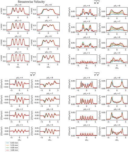
As shown in Fig. 3, predictions of velocity, $\overline{\mathit{v}\text{apos}v\text{apos}}$ and $\overline{\mathit{u}\text{apos}v\text{apos}}$, between the four meshes show extremely low mesh sensitivity. The results are practically indiscernible for most quantities and locations. The largest difference is visible in the $\overline{\mathit{u}\text{apos}u\text{apos}}$ predictions in the far field, while also noting that the difference is more noticeable due to the low value of the oscillations. The maximum error is less than 0.01 m²/s², which represents 20% of streamwise flow turbulence. This demonstrates that consistent predictions of mean velocity can be achieved even for the coarsest meshes (less than 2% change between the coarsest and finest mesh), while an intermediate mesh of 5.33 mm is sufficient to resolve unsteady oscillations in the main flow direction with some error in the transverse direction, still below 10% of the streamwise flow turbulence. The mesh requirements are consistent with previous findings by Lenci et al.,^[12] Xu,^[13] and Feng et al.^[15] These results point at mesh requirements on the order of 1/2 of the local ILSs between the base sizes of mesh 2 and mesh 3 listed Table III, resulting in an acceleration of approximately 100 times even for a stringent CFL = 1 requirement.

IV. RESULTS

IV.A. Mean Profiles

Mean velocity profiles computed by the STRUCT-ε simulations are compared to the experiment as well as the realizable k-ε turbulence model on the finest mesh discussed in the previous section, 3.00 mm. The realizable k-ε is used as a comparison to a commonly adopted industry solution.^[21] Figure 4 plots mean velocity profiles against experimental data sets.

Fig. 4. Mean streamwise velocity components plotted with experimental data sets.

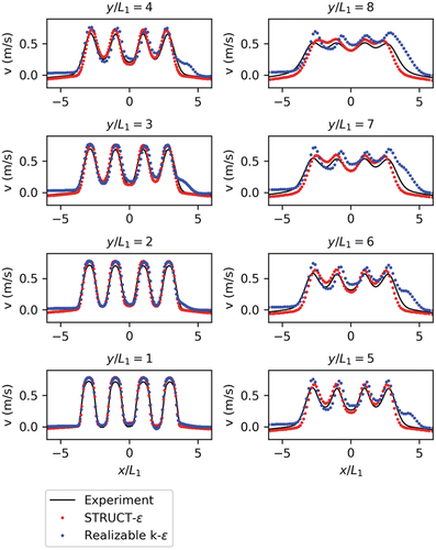
Velocity profiles computed by the STRUCT-ε solution match the experimental data with less than 4% error across the whole jet region from locations y/L₁ = 2 to 8, and less than 10% error on average overall. The predictions are most accurate near the jet inlets, while the largest error is produced as the jets converge in the far field. The realizable k-ε model shows larger differences, although a quantitative comparison is not applicable to this case as the model struggles to produce a symmetric solution for the flow configuration, which RANS models can suffer from as a consequence of the excessive turbulent viscosity predictions. The velocity profile leans to the right, becoming more severe farther from the inlet. While it might be possible in theory to force a symmetric solution for the realizable k-ε approach by adopting different solution approaches, the strong interaction of the model with the solution algorithms for these applications is an important limitation for industrial applicability. Further assessment of the asymmetric results was not pursued in this work as the model fails to reproduce the expected higher-frequency oscillations.

As the central feature being assessed is the ability of the models to predict the flow oscillations characteristic of thermal striping, mean profiles of Reynolds stresses $\overline{u^{\prime }{u}^{\prime }}$, $\overline{v^{\prime }{v}^{\prime }}$, and $\overline{u^{\prime }{v}^{\prime }}$ were further used to assess the performance of the STRUCT-ε turbulence model. Simulations using realizable k-ε are not shown in the assessment, as the realizable k-ε does not resolve any flow unsteadiness. Figure 5 plots the computed Reynolds stresses against the experiment.

Fig. 5. Mean Reynolds stresses plotted with experimental data sets.

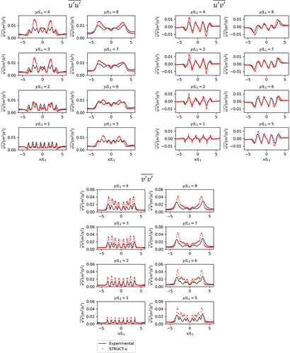
The results in Fig. 5 show consistent agreement in the predictions of Reynolds stress distributions. The STRUCT-ε model demonstrates the ability to resolve the most relevant unsteady flow structures, which are the most relevant characteristic for future applications to thermal striping assessment. For each of the Reynolds stresses plotted in Fig. 5, at y/L₁ = 1, STRUCT-ε captures the profiles well, while overestimating the quantitative values. Farther above the jet riser outlets, the peaks of the mean $\overline{v^{\prime }{v}^{\prime }}$ and $\overline{u^{\prime }{v}^{\prime }}$ profiles are overpredicted by STRUCT-ε, but the model still captures very similar trends. In the mean $\overline{u^{\prime }{u}^{\prime }}$, fewer peaks are resolved. It appears that two adjacent peaks merge into one larger peak. This can be seen at locations y/L₁ = 2, 3, 4, and 5. The overprediction of the turbulent stresses is an aspect that is being further investigated by comparison to high-fidelity LES,^[22] which also overpredict the experimental measurements.

IV.B. STRUCT-ε Model Activation

The activation of the hybrid resolution is key to the success of a generally applicable hybrid closure. As mentioned earlier, it is important to confirm that no spurious activations are produced in regions where the turbulence decay has larger influence, as this would lead to a degradation of the model predictions. For the STRUCT-ε model, the activation can be displayed by visualizing the additional turbulent dissipation rate ε source term. Figure 6 shows the log of the turbulent dissipation rate source on the measurement plane. Note that this is the instantaneous turbulent dissipation rate as opposed to a mean value.

Fig. 6. STRUCT-ε turbulence model activation identifying the four active jets in the selected test.

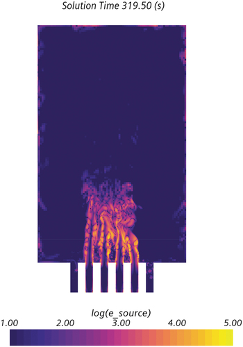
It is clear that STRUCT-ε activates in the region of the jet interaction. Because significant scale overlap is expected where the jets interact, this demonstrates that the STRUCT-ε model is working as intended.

IV.C. CFL Sensitivity Study

Using a higher CFL number could provide an even higher speed up from LES, which would benefit engineering tools for industrial applications. The sensitivity of the CFL number was tested on the second finest grid with a base size of 4 mm. The CFL number was varied based on the time step. CFL = 1 and CFL = 4 produced in the finest refinement region were tested. Figure 7 plots the streamwise velocity components $\overline{u^{\prime }{u}^{\prime }}$, $\overline{v^{\prime }{v}^{\prime }}$, and $\overline{u^{\prime }{v}^{\prime }}$.

Fig. 7. CFL sensitivity results from top left clockwise: streamwise velocity components $\overline{u^{\prime }{u}^{\prime }}$, $\overline{v^{\prime }{v}^{\prime }}$, and $\overline{u^{\prime }{v}^{\prime }}$.

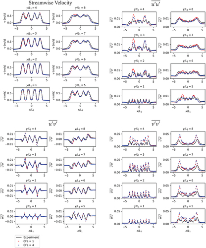
As shown in Fig. 7, CFL = 1 and CFL = 4 produce consistent predictions for velocity and Reynolds stresses. Similar to the results from the mesh sensitivity study, the difference is greatest in the cross-stream Reynolds stress profiles $\overline{u^{\prime }{u}^{\prime }}$. Both CFL = 1 and CFL = 4 result in slight asymmetry of the near field $\overline{u^{\prime }{u}^{\prime }}$ profiles, but the asymmetry is more pronounced for CFL = 4. Overall, simulations run with CFL = 1 and CFL = 4 show good agreement with experimentally measured data and provide consistent results. On this grid, CFL = 4 can provide 200 times the speed up from near wall–modeled LES, further demonstrating that STRUCT-ε can produce robust results for industrial applications.

V. CONCLUSIONS

This work assessed the applicability of the second-generation URANS turbulence model, STRUCT-ε, to the simulation of jet interaction, with the specific aim of assembling a robust modeling capability for thermal striping assessment. The results show that the model can accurately predict both the mean profiles of the streamwise velocity component, with less than 10% error across the jet region, as well as the Reynolds stresses ($\overline{u^{\prime }{u}^{\prime }}$, $\overline{v^{\prime }{v}^{\prime }}$, and $\overline{u^{\prime }{v}^{\prime }}$) at varying distances from the jet outlet. The resolution of the unsteady component of the flow is the most relevant aspect of the assessment in support of thermal striping applications.

As expected, the RANS approach, represented here by the realizable k-ε model, cannot capture any relevant unsteadiness because it does not resolve local fluctuations. Further, the realizable k-ε solution results in an asymmetric profile as a symptom of the incomplete physical representation, resulting in the overprediction of turbulent viscosity.

A key feature of the STRUCT-ε model is the consistent performance at varying grid resolutions, with less than 2% difference between the coarsest mesh and the finest mesh across the jet region, where the model confirmed the ability to provide high-quality predictions with an acceleration of approximately 100 times in comparison to the expected cost of a near wall–modeled LES solution. The consistency of the results is directly related to the ability of the model to only activate in regions of considerable scale overlap, independently from the local mesh resolution. Acceleration from near wall–modeled LES can be improved by increasing the CFL number. Sensitivity analysis of the CFL number showed that CFL = 1 and CFL = 4 can provide consistent results, reaching an overall acceleration factor of 200 from the LES solution.

The RCCS experiments provide valuable insight into the performance of STRUCT-ε, and further, provide a reference configuration leveraged by the research team at Penn State University^[22] to produce high-resolution LES diabatic simulations to fully assess STRUCT-ε for thermal striping applications. Continued evaluation of STRUCT-ε with varying test cases is being performed^[23] to further the maturity of this tool for industry applications.

Acknowledgments

This work was funded by a U.S. Department of Energy Integrated Research Project “Center of Excellence for Thermal-Fluids Applications in Nuclear Energy: Establishing the knowledgebase for thermal-hydraulic multiscale simulation to accelerate the deployment of advanced reactors,” IRP-NEAMS-1.1: Thermal-Fluids Applications in Nuclear Energy. This work was completed with support and guidance from TerraPower LLC. The authors report there are no competing interests to declare.

Disclosure Statement

No potential conflict of interest was reported by the authors.

References

- O. GELINEAU and M. SPERANDIO, “Thermal Fluctuation Problems Encountered in LMFBRs, IAEA-IWGFR/90,” presented at the Specialistic Mtg. on Correlation Between Material Properties and Thermohydraulics Conditions in LMFBRs, Aix-en-Provence, France (1994).
- C. BETTES, A. M. JUDD, and W. W. J. LEWIS, “Avoiding Thermal Striping Damage: Experimentally Based Design Procedures for High Cycle Thermal Fatigue, IWGFR/90,” presented at the Specialistic Mtg. on Correlation Between Material Properties and Thermohydraulics Conditions in LMFBRs, Aix-en-Provence, France (1994).
- V. A. SOBOLEV and N. G. KUZAVKOV, “Identification of Places with Fluid Temperatures in BN 600 Reactor and Reactor Systems, IAEA-IWGFR/90,” presented at the Specialists Mtg. on Correlation Between Material Properties and Thermohydraulics Conditions in LMFBRs, Aix-en-Provence, France (1994).
- P. JUNGCLAUS, D. VOSWINKEL, and A. NEGRI, “Common IPSN/GRS Safety Assessment of Primary Coolant Un-isolable Leak Incidents Caused by Stress Cycling,” International Atomic Energy Agency (1998).
- C. FAIDY et al., “Thermal Fatigue in French RHR System,” presented at the Int. Conf. on Fatigue of Reactor Components (2000).
- C. J. LAWN, “The Attenuation of Temperature Oscillations by Liquid Metal Boundary L Layers,” Nucl. Eng. Des., 42, 2, 209 (1977); https://doi.org/10.1016/0029-5493(77)90182-0.
- T. MURAMATSU and H. NINOKATA, “Development of Thermohydraulics Computer Programs for Thermal Striping Phenomena,” Nucl. Tech., 113, 1, 54 (1996); https://doi.org/10.13182/NT96-A35199.
- P. R. SPALART, “Strategies for Turbulence Modelling and Simulations,” Int. J. Heat Fluid Flow, 21, 3, 252 (2000); https://doi.org/10.1016/S0142-727X(00)00007-2.
- F. R. MENTER and Y. EGOROV, “A Scale-Adaptive Simulation Model Using Two-Equation Models,” presented at the 43rd AIAA Aerospace Sciences Meeting and Exhibit—Meeting Papers, 271, American Institute of Aeronautics and Astronautics Inc. (2005); https://doi.org/10.2514/6.2005-1095.
- B. L. SMITH, J. H. MAHAFFY, and K. ANGELE, “A CFD Benchmarking Exercise Based on Flow Mixing in a T-junction,” Nucl. Eng. Des., 264, 80 (2013); https://doi.org/10.1016/J.NUCENGDES.2013.02.030.
- G. LENCI, “A Methodology Based on Local Resolution of Turbulent Structures for Effective Modeling of Unsteady Flows,” Massachusetts Institute of Technology (2016).
- G. LENCI, J. FENG, and E. BAGLIETTO, “A Generally Applicable Hybrid Unsteady Reynolds-Averaged Navier-Stokes Closure Scaled by Turbulent Structures,” Phys. Fluids, 33, 105117 (2021); https://doi.org/10.1063/5.0065203.
- L. XU, “A Second Generation URANS Approach for Application to Aerodynamic Design and Optimization in the Automotive Industry,” Massachusetts Institute of Technology (2020).
- J. GARCÍA et al., “A Second-Generation URANS Model (STRUCT-ε) Applied to Simplified Freight Trains,” J. Wind Eng. Ind. Aerodyn., 205, 104327 (2020); https://doi.org/10.1016/J.JWEIA.2020.104327.
- J. FENG, T. FRAHI, and E. BAGLIETTO, “STRUCTure-Based URANS Simulations of Thermal Mixing in T-Junctions,” Nucl. Eng. Des., 340, 275 (2018); https://doi.org/10.1016/j.nucengdes.2018.10.002.
- J. ACIERNO and E. MERZARI, “On the Role of Low Frequency Modes in the Thermal and Momentum Mixing in Parallel Plane Jets,” SSRN Electron. J. (2022); https://doi.org/10.2139/ssrn.4314495.
- D. D. LISOWSKI et al., “Final Project Report on RCCS Testing with Air-Based NSTF,” ANL-ART-47, Argonne National Laboratory (2016); https://doi.org/10.2172/1350591.
- D. NUNEZ et al., “Modal Analysis of Parallel Rectangular Jets Interactions in the RCCS Separate-Effects Test Facility,” presented at the 18th Int. Topl. Mtg. on Nuclear Reactor Thermal Hydraulics (NURETH-18), Portland, Oregon (2019).
- D. NUNEZ, “High-Resolution Experiments of Momentum- and Buoyancy-Driven Flows for the Validation and Advancement of Computational Fluid Dynamics Codes,” University of Michigan (2020).
- N.-S. LIU and T.-H. SHIH, “Turbulence Modeling for Very Large-Eddy Simulation,” AIAA J., 44, 4, 687 (2006); https://doi.org/10.2514/1.14452.
- M. REHM, A. HATMAN, and B. FARGES, “Framatome’s Unified Single-Phase CFD Methodology for Fuel Design and Analysis,” Proc. CFD4NRS-8, Virtual Conf., p. 25 (2020).
- J. ACIERNO and E. MERZARI, “Large Eddy Simulation of Jet Interaction,” p. 1, Advances in Thermal Hydraulics (2022).
- E. BAGLIETTO et al., “Challenge Problem 2: Benchmark Specifications for Thermal Striping of Reactor Internals,” ANL/NSE-21/18, Argonne National Laboratory (2021).