Optimizing the Implementation of Small Modular Reactors into Ontario’s Future Energy Mix

Abstract

This paper performs a detailed analysis of the optimized Ontario power mix under impending load and emissions constraints with the consideration of small modular reactor (SMR) deployment. The target of minimizing the total cost of the 2055 power mix while retaining real-world energy requirements was achieved using a semidynamic, recursive linear optimization model with hourly time resolution for the accurate consideration of wind and photovoltaic variable renewable energy. Utilizing IBM’s ILOG CPLEX Optimization Studio’s Flow Control method, dynamic factors such as forecasted demand growth, increasing capacity installations, learning curve applications, and reactor refurbishment and decommissioning schedules were applied to the modeling scenarios. Optimized scenarios have demonstrated that SMR-based capacity should play a vital role in the provincial energy mix in order to minimize cost while meeting emissions reduction goals and responding to increasing demand. Simulations show ideal cost reductions when approximately one-third of generated energy is produced by SMRs in the future energy mix and that the absence of SMRs may lead to up to 29% higher spending. Additional cases have considered the benefits of early SMR investment and direct SMR-CANDU cost comparisons.

Keywords:

• Small modular reactors
• Ontario energy mix
• linear programming
• recursive optimization
• learning curve

I. INTRODUCTION

In recent decades, the nuclear industry and market for reactors have begun to make a shift from large, costly reactors to smaller, more manageable projects to make the industry more sustainable, safer, economical, and farther reaching.^[1] Among such shifts has been the emergence of small modular reactors (SMRs) as a viable new technology, allowing significant variability in size and power output, notable reductions in capital investments, and drastic technological advances with next-generation designs and fuels. The Canadian Small Modular Reactor Roadmap Steering Committee identified three primary areas of application in its report: urban, on grid (largest SMRs, replacing coal and fossil fuel plants); off grid (micro SMRs for rural areas, replacing large diesel generators); and on-and-off grid (variable size, replacing heating and diesel generators in industrial areas).^[1]

In its current position, the Canadian nuclear industry has embraced the introduction of SMRs, noting that it stands well-suited to take a firm step into the SMR market, applying next-generation technology throughout the country to meet its clean energy needs and becoming a global leader in a rapidly growing industry. However, despite the commitment from several provinces to the development of an initial wave of SMR technology, little attention has been paid to the long-term impact of introducing a new utility to the existing provincial energy mixes. In the context of Ontario, it is unclear how a province operating with a surplus energy capacity will embrace a yet-unproven technology. Many existing studies have presented a wide range of static projected costs for SMRs, with some considering both early and later stages but providing minimal information regarding the relationship between cost and installed capacity. Though useful, these studies tend to fall short of considering the impact that price variations will have on the scale of SMR deployment, and as a result, their economic viability remains a major area of uncertainty.^[2,3]

On the front end, SMRs do appear to have the potential to be economically competitive. They require a significantly lower capital investment than large-scale reactors due to the uniform reductions in size, construction requirements, and material cost.^[4] Further, their relatively small size and the modularity of their application (e.g., a large reactor site may be replaced by a set of identical SMRs for an equal total installed capacity) allow for factory-style construction. This potentially reduces the cost per kilowatt (as repeatability allows for assembly line–style construction); increases safety (increased consistency in construction); and allows for a less resource-intensive process, as newly constructed reactors can provide power for the construction of subsequent modules.^[1,3] Finally, the introduction of small-scale reactors allows space for innovative new reactor designs that boast better fuel efficiency and potential waste reductions while increasing safety by implementing passive cooling and emergency systems.^[1] Favorable initial projections for SMR costs expect that annualized capital costs per kilowatt will be comparable to that of traditional reactors due to the lack of experience in production for the first wave of SMRs.^[4] However, as production methods gain practice and become standardized, the learning curve is expected to drop the cost per kilowatt well below that of comparable utility types, following the standard n’th-of-a-kind (NOAK) or learning curve cost models.^[5]

On a national scale, Canada is roughly 25% of the way to meeting its greenhouse gas (GHG) reduction goal set in the Paris Agreement solely from the use of Ontario’s existing nuclear installations.^[2] The current reactor fleet avoids the production of approximately 50 million tonnes of carbon dioxide every year,^[2] though Canada is still expected to fall short of its emission reduction goals. For the development of a sustainable system that will allow Canada to reach its targets, a balance must be maintained among investment into net zero generation strategies, supporting demand growth, and maintaining energy diversity and security. If the economic viability of SMRs may be demonstrated, they could play a pivotal role as a new technology that is both scalable and non-carbon emitting. Such a demonstration requires the employment of an energy system model that can consider the existing power mix, future demand growth, environmental constraints, and economic considerations.

Based on this assessment, this paper investigates the economically optimized 2055 power mix for Ontario under a collection of real-world constraints. The distinction was made to specifically analyze the Ontario power mix due to the separation of provincial energy policies, and the analysis was conducted using a linear optimization model. As of 2022, Ontario’s energy mix comprises essentially six main resources, five of which are carbon neutral: nuclear (CANDU), natural gas, hydroelectricity,^a wind, photovoltaics (PV), and biomass.^[6] Over the next 20 years, the provincial demand for electricity is expected to increase by approximately 1.7%/yr following past trends as reference.^[6] In terms of net energy demand, this translates to a growth of 56 TW∙h, from 147 TW∙h in 2023 to 202 TW∙h by 2042.^[6,7] The projection from the 2021 Annual Planning Outlook (APO) describes how the summer and winter peak demands are expected to increase at the same rate, reaching approximately 31.5 and 30.5 GW in the 2042 standard reference case, respectively.^[7] Simultaneously, because of the large number of nuclear refurbishments required at the Darlington and Bruce generating facilities between 2020 and 2035, as well as the scheduled retirement of Pickering’s six units in 2024 and 2025, Ontario’s total installed capacity is expected to fluctuate significantly. These reductions are expected to drop the total provincial capacity to as low as 37 GW in the late 2020s before leveling to 40 GW by the mid-2030s,^[6] which is an overall reduction from the current value despite increasing demand. In its current state, it is expected that reserve supply will come from additional natural gas capacity, increasing annual emissions.

II. MATHEMATICAL MODELING

II.A. Linear Programming

A subset of mathematical programming, linear programming is one of the simplest methods of optimization. Given a set of decision variables and subject to constraints defined by linear equalities and/or inequalities, a linear objective function may be optimized to find its maximum or minimum values. A feasibility region is first created by the function, whose boundaries are defined by the linear constraints, and each point along which represents a possible solution corresponding to varying values for the decision variables. In most practical situations, the number of decision variables can grow very quickly depending on the system that is being modeled. The Simplex method is an iterative process for solving linear programming problems, where the values of the decision variables are sequentially tested until an optimal solution is found. This method involves writing the objective function in the form

(1) $\begin{array}{c}Z\left(x\right)=C_1{x}_1+C_2{x}_2+\dots +C_n{x}_n\end{array},$(1)

where $Z\left(x\right)$ = objective function, $C_n$ = defined constants, and x = a vector array of decision variables $x_1,\dots ,x_n$. It follows that the constraints can be written as the matrix equation:

(2) $\begin{array}{c}\mathbf{A}\mathbf{x}=\mathbf{B}\end{array},$(2)

where A = matrix made up of the predefined constants in the linear constraints, $a_{11},\dots ,a_{mn}$, and B = matrix comprising the constraint values, $b_1,\dots ,b_m$, which can be either a defined constant or a decision variable value.^[8] In this form, both $x_n$ and $b_m$ must be greater than 0. This restriction is referred to as the nonnegativity restriction, which states that for all linear programs, the decision variables should always take nonnegative values in order to ensure real solutions.^[8]

Given the nature of such models, the above matrix can quickly become overwhelming as more decision variables and constraints are introduced to generate a more realistic model. For these reasons, it is common practice to use specialized software to solve large-scale linear programming problems more quickly and reliably.

II.A.1. IBM’s ILOG CPLEX Optimization Studio

For the purpose of this investigation, IBM’s ILOG CPLEX Optimization Studio, henceforth referred to as CPLEX, was used. This system utilizes IBM’s “intelligent software” (ILOG) and the application of the aforementioned Simplex method via C programming language. CPLEX allows for the simple creation and solving of a linear optimization model, requiring only defined decision variables, linear constraints, and an objective function, in addition to the relevant input values (applied as coefficients). For this model, the barrier method and CPLEX’s Flow Control (see Sec. A.I of the Appendix) were applied to solve the model.

II.B. CPLEX Model

With the proposed introduction of SMRs into Canada, the introduction of said technology into Ontario’s energy mix is an ideal candidate for investigation. Using linear programming, this model represents Ontario’s implementation of SMRs over an initial 33-year period, allowing for consideration of Ontario’s current energy mix as well as the potential for multiple generations of SMR installations.^[1] In its current form, the model seeks to minimize the overall future cost of electricity production in Ontario by considering the installation of SMR-based capacity as a seventh carbon neutral source of electricity generation (eighth total source, following those discussed in Sec. II).

The model begins by considering the current energy mix and accounting for Ontario’s approximately 40.5 GW of installed capacity.^[7] The existing capacity for each of the seven real resources is inputted as a constant, having no initial construction costs included other than those associated with power production, thus ensuring that the starting point for the program reflects reality. In the case of the eighth resource, SMRs, the minimum installed value is left at 0 MW as there are no operational commercial SMRs yet installed in Ontario. There are three primary decision variables in the model: $k{n}_j$, representing the optimal amount of new capacity for the model to install, per plant type; k_j, representing the optimal total amount of installed capacity (preexisting capacity plus new capacity $k{n}_j$) for each power plant type j; and x_ji, representing the power output for each resource j at each time step i. All endogenous and exogenous variables and their descriptions may be found in Tables I and II. There are eight power plant types, and the time steps are hourly. Secondary definitions may be found in Table A.I of the Appendix.

TABLE I Endogenous Variables in CPLEX Model

TC	Total cost of model instance period ($/period)
K0, j	Preexisting capacity of j’th-type power plant within provincial energy mix when model instance initiates (kW)
GhgEmj	CO2 emissions for j’th-type power plant (gCO2/kW∙h)
CFj	Capacity factor for j’th-type power plant
knj	Newly installed capacity by model for j’th-type power plant (kW)
kj	Total installed capacity, preexisting and new, for j’th-type power plant (kW)
xi, j	Energy output during i’th time step for j’th-type power plant (kW∙h)
i	i ∈ {1, 2, 3, …, Years} Years: number of hours in a model instance (3 years = 26 280 h)
PlantTypej	PlantTypej ∈ {1: CANDU-based nuclear, 2: large hydropower, 3: small hydropower, 4: wind, 5: PV, 6: natural gas, 7: biomass/Other, 8: SMR-based nuclear}
a, b, c, d, e, f, g, h	Total energy output by each power plant (a = 1, … h = 8) during model instance (kW∙h)
j	j ∈ {1, 2, 3, …, N} N: Number of plant types in model instance
Accumj	Accumulating variable for j’th plant type, used to track iterations for later in postprocessing

TABLE II Exogenous Variables in CPLEX Model

FCRj	The annual fixed charge rate of the j’th power plant
Loadi	Demand on power grid during i’th time step (kW)
Fixedj	Sum of annual fixed costs for j’th-type power plant ($/kW∙yr)
Variablej	Sum of variable cost for j’th-type power plant ($/kW∙h)
CTn	Carbon tax for j’th-type power plant ($/kW∙h)
MaxCapj	Maximum installable capacity value based on remaining potential and preexisting capacities of j’th-type power plant (kW)
CapLimj	Available capacity limit (kW)
PVAvailabilityj	Hourly availability profile of PV potential, based on favorable yearly weather profile for Ontario
WindAvailabilityj	Hourly availability profile of wind potential, based on favorable yearly wind profile for Ontario
EmLim	Total annual CO2 emissions limit allowed by provincial regulations (g CO2/kW∙h)
MaxLoad	Maximum load demand in single hour across all time steps in model instance (kW)
CapRM	Capacity reserve margin, typically valued from 10% to 15% depending on demand throughout year
K0,1’, K0,1”, K0,1”’	Installed CANDU capacity variations
σ	Average expected transmission losses
ζ	Projected demand increase for model instance
Φmax,j, Φmin,j	Minimum and maximum output power levels, respectively, for j’th power plant
δI,j, δD,j	Maximum increase and decrease rate of changes of power outputs for j’th power plant, respectively
λ	Effective CANDU capacity reducing factor
Ωn	Milestone capacity values for application of NOAK cost reductions to SMR installed capacity
α	NOAK coefficient for cost reductions
n	Postprocessing counter, where n ∈ {1, 2, 3, 4}
Spring	Ranges of i corresponding to three spring seasons during model period: i ∈ {1896, …, 4086}, {10656 … 12846}, {19416 … 21606}
Fall	Ranges of i corresponding to three fall seasons during model period: i ∈ {6276 … 8466}, {15036 … 17226}, {23796 … 25986}

II.B.1. Objective Function

The objective function for the model is a summation of the respective costs for the initial construction and ongoing usage of each power plant type throughout the forecast period of a single model instance. These values are represented by the fixed and variable costs for each power plant type, as can be seen in Eq. (3)(3) $\begin{array}{rlr}& TC=\sum _{j=1}^8\left[FC{R}_j\times P{F}_j\times k_j+\sum _{i=1}^{Years}{x}_{ji}\left[P{V}_{ji}+C{T}_j\right]\right].& (3)\end{array}$(3) . These costs are inputted as values of cost per kilowatt or cost per kilowatt hour. The objective function is of the form

(3) $\begin{array}{rlr}& TC=\sum _{j=1}^8\left[FC{R}_j\times P{F}_j\times k_j+\sum _{i=1}^{Years}{x}_{ji}\left[P{V}_{ji}+C{T}_j\right]\right].& (3)\end{array}$(3)

The input values $P{F}_j$ and $P{V}_{ji}$ representing the fixed and variable costs, respectively, are multiplied by their associative decision variables k_j and x_ji to create the above objective function that expresses the total cost TC of all power plant types j over all time steps i. Here, $FC{R}_j$ is the annual fixed charge rate of the j’th power plant.^[1]

The model seeks to optimize the economic effect of introducing a new power plant type versus simply increasing the installed capacity of the existing types by applying the previously discussed Simplex method to minimize TC. The associated cost values account for the annualized fixed costs, including the overnight capital cost (OCC) and fixed operation and maintenance (O&M) costs; the variable costs, including variable O&M costs, fuel cost, and transmission costs; and additional supplemental costs, including transmission line construction and carbon tax (refer to Table III). These values are inputted as arrays of constants of length j, with each value corresponding to its respective plant type, as can be seen in Table II.

TABLE III Exogenous Variable Input Values for Various Power Plant Types

	Nuclear (CANDU)	Hydropower (Large)	Hydropower (Small)	Natural Gas	Biomass	SMR (GE Hitachi)	SMR (NuScale)
CPLEX Input Arrays	j = 1	j = 2	j = 3	j = 6	j = 7	j = 8	j = 8
Overnight capital cost ($/kW)	6276	6160	6930	1433	4650	3400	4000
Lifetime (yr)	30	30	30	20	30	60	60
Fixed O&M ($/kW∙yr^−1)	125.37	92	100	18.25	116	148.79	145
Annual fixed cost (¢/kW∙yr^−1)	33 457	29 733.33	33 100	8990	27 100	20 545.53	22 083.33
Variable O&M cost (¢/kW∙h)	0	0.33	1.67	0.28	0.18	0.10	0.095
Rate of output maximum increase (1/h)	0.60	0.05	0.05	0.44	0.31	0.60	0.60
Rate of output maximum decrease (1/h)	0.60	0.05	0.05	0.31	0.58	0.60	0.60
Fuel cost (¢/kW∙h)	1.45^a	0	0	2.44	2.16	1.10^a	1.10^a
Transmission costs (¢/kW∙h)	0	0.15	0.15	0	0.15	0	0
Total variable unit cost (¢/kW∙h)	1.45	0.48	1.82	2.72	2.49	1.20	1.20
Carbon tax (¢/kW∙h)	0	0	0	1.77	0	0	0
	Wind	PV
CPLEX Input Arrays	j = 4	j = 5
Overnight capital cost ($/kW)	2600	2140
Lifetime (yr)	20	20
Fixed O&M ($/kW∙yr^−1)	23	26
Annual fixed cost (¢/kW∙yr^−1)	15 300	13 300
Variable O&M cost (¢/kW∙h)	0	0
Fuel cost (¢/kW∙h)	0	0
Transmission costs (¢/kW∙h)	0.15	0.15
Total variable unit cost (¢/kW∙h)	0.15	0.15
Carbon tax (¢/kW∙h)	0	0

*References 2, 11, 14, 21, 29, and 32.

^aFuel cost includes 10 ¢/kW for future disposal.

The annual fixed charge rate represents the fraction of the total power plant cost that is required each year over the lifetime of the power plant to meet the minimum annual revenue requirements.^[1] It is expressed as

(4) $\begin{array}{rl}FC{R}_j=\left[\begin{array}{c}\frac{1-r_j}{n_j}+i+tax+om{r}_j-\\ \frac{1-r_j}{n_j}\left(i+tax\right)\left(\frac{1}{i}-\frac{n_j}{{\left(1+i\right)}^{n_j}-1}\right)\end{array}\right]\text{vskip}20,& \text{vskip}20(4)\end{array}$(4)

where $r_j$ = scrap value ratio at the end of the power plant’s lifetime, $n_j$ = lifetime of the power plant, $i$ = annual interest rate, $tax$ = annual property tax rate for Ontario, and $om{r}_j$ = annual fixed O&M cost ratio to initial investment.^[2] The interest rate in this paper is assumed as 4%.

II.B.2. Linear Constraints

II.B.2.a. Power Supply and Demand Constraints

The necessary relationship between the power demands by the public, represented by Load_i and generated from 2020 Independent Electricity System Operator (IESO) data,^[3] and the collective output supply from eight power plants is governed by Eq. (5)(5) $\begin{array}{c}\sum _{j=1}^8(x_{ji}-\sigma x_{ji})=Loa{d}_i\mathrm{\forall }i.\end{array}$(5) :

(5) $\begin{array}{c}\sum _{j=1}^8(x_{ji}-\sigma x_{ji})=Loa{d}_i\mathrm{\forall }i.\end{array}$(5)

An estimated average transmission loss of 4% has been accounted for.^[2] Equations (6)(6) $\begin{array}{c}{k}_j=K_{0,j}+k{n}_j\mathrm{\forall }i\end{array}$(6) , (7)(7) $\begin{array}{c}{k}_j\le MaxCa{p}_j\mathrm{\forall }j\end{array}$(7) , and (8)(8) $\begin{array}{c}{k}_2+k_3\le MaxCa{p}_{2,3}\end{array}.$(8) define the total capacity as the combination of preexisting capacities and the newly constructed capacities and define the upper boundary for all capacities:

(6) $\begin{array}{c}{k}_j=K_{0,j}+k{n}_j\mathrm{\forall }i\end{array}$(6)

(7) $\begin{array}{c}{k}_j\le MaxCa{p}_j\mathrm{\forall }j\end{array}$(7)

(8) $\begin{array}{c}{k}_2+k_3\le MaxCa{p}_{2,3}\end{array}.$(8)

As the remaining hydroelectric potential in Ontario is a combination of small and large hydropower, the combination of these total capacities ($k_2+k_3$) is constrained by the value of the upper boundary.^[4] The capacity factor is defined for the model in Eq. (9)(9) $\begin{array}{c}C{F}_j\left(k_j\times Years\right)\ge \sum _{i=1}^{Years}{x}_{ij}\mathrm{\forall }j.\end{array}$(9) :

(9) $\begin{array}{c}C{F}_j\left(k_j\times Years\right)\ge \sum _{i=1}^{Years}{x}_{ij}\mathrm{\forall }j.\end{array}$(9)

The maximum installable capacities for wind and PV have been set to infinity due to the significant remaining potential and area for expansion for these technologies. As the model does not opt to build any significant amounts of natural gas capacity due to the intense carbon tax with or without a maximum potential value, this too was set to infinity. The maximum installable biomass potential was set to 1600 MW.^[5] Because of uncertainty regarding the future of nuclear development projects and specific capacity targets in Ontario, the CANDU and SMR maximum capacities have been left open-ended (infinity placeholder values).^[6] The variations in currently installed capacity due to refurbishments and decommissioning are addressed below.

II.B.2.b. Operational Window Constraints

The operational window for power output from all power plants is governed by Eqs. (10)(10) $\begin{array}{c}{x}_{j,i}\ge {\phi }_{min,j}{k}_j\mathrm{\forall }i\end{array}$(10) and (11)(11) $\begin{array}{c}{x}_{j,i}\le {\phi }_{max,j}{k}_j\mathrm{\forall }i.\end{array}$(11) :

(10) $\begin{array}{c}{x}_{j,i}\ge {\phi }_{min,j}{k}_j\mathrm{\forall }i\end{array}$(10)

(11) $\begin{array}{c}{x}_{j,i}\le {\phi }_{max,j}{k}_j\mathrm{\forall }i.\end{array}$(11)

The operational window for CANDU $x_{1,i}$ has been established using IESO data from 2019 and 2020 on the standard operational outputs of Ontario’s existing nuclear fleet.^[7] The hourly availability profiles of wind and PV potential are generated from region-specific hourly weather data year-to-year^[8]:

(12) $\begin{array}{c}{x}_{4,i}\le C{F}_4\times WindAvailabilit{y}_i\mathrm{\forall }i\end{array}$(12)

(13) $\begin{array}{c}{x}_{5,i}\le C{F}_5\times PVAvailabilit{y}_i\mathrm{\forall }i\end{array}.$(13)

The minimum safe operating power level of 15% to 30% full power (%FP) for advanced light water reactors (LWRs) was applied to the SMR estimate $x_{8,i}$,^[9] with a conservative narrowing of the operational range by 10%.

II.B.2.c. Power Output Rate of Change Constraints

For the purposes of load-following or “hole filling” power output processes, the following constraints govern the operational flexibility of each power plant with regard to the derivative of its output power:

(14) $\begin{array}{c}{x}_{j,i+1}\le {\delta }_{I,j}{x}_{j,i}\mathrm{\forall }i\end{array}$(14)

(15) $\begin{array}{c}{x}_{1,i+1}\ge {\delta }_{D,j}{x}_{j,i}\mathrm{\forall }i\end{array}.$(15)

As with LWRs, CANDU reactors are considered flexible and capable of load-following when operating within a power range of 60% to 100% FP.^[10] Natural gas–based, biomass-based, and oil-based capacities share the advantage of being flexible, hole filling utilities, capable of load-following or supplementing a baseload power source.^[11] The assigned value of ±60% for SMR hourly operational flexibility is based on the known flexibility of current LWRs and is considered a conservative assumption.^[10,12]

II.B.2.d. Capacity Reserve Constraint

The capacity reserve constraint for this model is 15%. Common values for capacity reserve constraints vary between 10% and 25%^[13]:

(16) $\begin{array}{c}\sum _{j=1}^8{k}_j\times C{F}_j\ge \left(1+CapRM\right)MaxLoad\end{array}.$(16)

II.B.2.e. CO₂ Constraint

$EmLim$ represents the provincial regulations regarding annual maximum CO₂ emissions and constraints emissions to this upper boundary for each year of the 3-year model instance^[12,14]:

(17) $\begin{array}{c}\sum _{j=1}^8\sum _{i=1}^{Yea{r}_1}{x}_{ji}\times GhgE{m}_j\le EmLim\end{array}$(17)

(18) $\begin{array}{c}\sum _{j=1}^8\sum _{i=Yea{r}_1}^{Yea{r}_2}{x}_{ji}\times GhgE{m}_j\le EmLim\end{array}$(18)

(19) $\begin{array}{c}\sum _{j=1}^8\sum _{i=Yea{r}_2}^{Yea{r}_3}{x}_{ji}\times GhgE{m}_j\le EmLim\end{array}.$(19)

II.B.2.f. CANDU Scheduled Seasonal Outages

The current frequency of scheduled outages for modern CANDU reactors is 21 days every 2 years.^[15] Given the number of operational CANDU reactors in Ontario, this equates to approximately 1 accumulative-year of a single reactor undergoing a scheduled outage in a 2-year period, or 1.5 years in a 3-year period. Constraints (20) and (21) reduce the effective operational capacity of the nuclear (CANDU) power plant accordingly:

(20) $\begin{array}{c}{x}_{1,i}\le \lambda k_{1}i=\left\{spring\right\}\end{array}$(20)

(21) $\begin{array}{c}{x}_{1,i}\le \lambda k_{1}i=\left\{fall\right\}\end{array}.$(21)

Appropriate indexing has been applied to confine these reductions in capacity to the spring and fall periods, outside of peak power demand months.^[15]

II.B.3. Flow Control Postprocessing

The postprocessing feature of Flow Control allows for data acquisition and editing before or following each model instance. This process is used to update a number of exogenous variable values, transfer data from previous model instances, and apply realistic constraint changes between subsequent model instances. The postprocessing feature allows the model to shift from purely static to a Flow Control–driven, semidynamic model by applying time-based variations.^[16]

II.B.3.a. Installed Capacity Update

Following each model instance, the preexisting capacities $K_{0,j}$ must be updated to include the newly added capacities from the completed model instance. Equation (22)(22) $\begin{array}{c}{K}_{0,j}=k_j\mathrm{\forall }j\end{array}.$(22) performs this action such that the subsequent model instance initiates with $K_{0,j}$ values corresponding to the total installed capacity per plant type from the previous model instance:

(22) $\begin{array}{c}{K}_{0,j}=k_j\mathrm{\forall }j\end{array}.$(22)

II.B.3.b. Power Demand Growth

In December 2021, the IESO’s APO projected an average increase in provincial power demand of approximately 1.7% annually over a 20-year period^[6]:

(23) $\begin{array}{c}Loa{d}_i=\zeta Loa{d}_i\mathrm{\forall }i\end{array}.$(23)

Figure 1 provides a visual reference for the magnitude of this demand increase as it applies to the two primary annual peaks. This paper assumes that this trend will remain relatively steady and may be extrapolated an additional 13 years, totaling a 33-year period. The approximate average annual demand growth has increased incrementally year-to-year in the 2019, 2020, and 2021 APOs (0.9%, 1%, and 1.7%, respectively); thus, this extrapolation is considered to be a conservative assumption.^[6,17,18]

Fig. 1. Projected demand curve for peak summer and winter demand over 20-year period from IESO’s 2021 annual planning outlook.^[6]

II.B.3.c. Application of NOAK Costs

Factory-style fabrication, development of global supply chains, and the learning curve of production techniques are projected to have significant effects on the NOAK cost reductions of SMR projects relative to first-of-a-kind (FOAK) costs.^[19] Typical results for learning curve and NOAK cost predictions follow a 5% to 10% reduction in cost per doubling of installed SMR capacity globally.^[19–21] These reductions are applied incrementally to the model instances as the SMR capacity values set by the model pass the milestone values indicated in Eq. (24)(24) $\begin{array}{rl}& \mathrm{i}\mathrm{f}\left(K_{0,8}\ge {\mathrm{\Omega }}_n\right):\\ & \left\{\begin{array}{c}Fixe{d}_8=\left(1-\alpha n\right)Fixe{d}_8,\\ Variabl{e}_8=\left(1-\alpha n\right)Variabl{e}_8\end{array}\right\}\text{vskip}8.& \text{vskip}8(24)\end{array}$(24) :

(24) $\begin{array}{rl}& \mathrm{i}\mathrm{f}\left(K_{0,8}\ge {\mathrm{\Omega }}_n\right):\\ & \left\{\begin{array}{c}Fixe{d}_8=\left(1-\alpha n\right)Fixe{d}_8,\\ Variabl{e}_8=\left(1-\alpha n\right)Variabl{e}_8\end{array}\right\}\text{vskip}8.& \text{vskip}8(24)\end{array}$(24)

II.B.3.d. Application of Federal Carbon Tax, CANDU Refurbishments, and Decommissioning

As of 2022, the Canadian federal carbon tax is $50/tonne CO₂ and is intended to increase by $15/tonne CO₂ annually until it reaches a ceiling of $170/tonne CO₂.^[14] Because of the linear annual increase, the average carbon tax across the 3-year period of each model instance may be used to accurately represent the total cost per tonne CO₂. With each model instance and corresponding 3-year period, the carbon tax is increased to a new average value until the ceiling value of $170/tonne CO₂ is achieved, at which time this value remains constant. Ontario’s existing nuclear capacity is currently experiencing variations as portions of the CANDU fleet undergo scheduled refurbishments or decommissioning.^[22,23]

The scheduled reductions in installed capacity (Fig. 2) are applied to the corresponding model instance by varying the value of $K_{0,1}$, as seen in Eqs. (25)(25) $\begin{array}{rl}& \mathrm{i}\mathrm{f}\left(Accu{m}_1==n\right):\\ & \left\{\begin{array}{c}C{T}_n=C{T}_{n+1},\\ K_{0,1}=K_{0,1}^{\prime }\\ n=n+1\end{array}\right\}& \text{vskip}15(25)\end{array}$(25) and (26)(26) $\begin{array}{rl}& \mathrm{e}\mathrm{l}\mathrm{s}\mathrm{e}\mathrm{i}\mathrm{f}\left(Accu{m}_1\ge n\right):\\ & \left\{\begin{array}{c}CT=C{T}_4\\ K_{0,1}=K_{0,1}^{{ }^{\prime \prime }}\end{array}\right\}\text{vskip}10.& \text{vskip}10(26)\end{array}.$(26) , such that the initial installed capacity of each model instance aligns approximately with the above schedule:

(25) $\begin{array}{rl}& \mathrm{i}\mathrm{f}\left(Accu{m}_1==n\right):\\ & \left\{\begin{array}{c}C{T}_n=C{T}_{n+1},\\ K_{0,1}=K_{0,1}^{\prime }\\ n=n+1\end{array}\right\}& \text{vskip}15(25)\end{array}$(25)

(26) $\begin{array}{rl}& \mathrm{e}\mathrm{l}\mathrm{s}\mathrm{e}\mathrm{i}\mathrm{f}\left(Accu{m}_1\ge n\right):\\ & \left\{\begin{array}{c}CT=C{T}_4\\ K_{0,1}=K_{0,1}^{{ }^{\prime \prime }}\end{array}\right\}\text{vskip}10.& \text{vskip}10(26)\end{array}.$(26)

Fig. 2. CANDU reactor refurbishment and decommissioning schedule.^[6]

II.B.4. Model Assumptions

Despite the nationwide endeavor to adopt SMRs into the Canadian energy mix, this investigation has been limited to the Ontario energy mix. This restriction reduces the diversity of the energy mix in question, allows primarily urban SMR implementation to be considered, and greatly reduces the number of constraints required to generate a realistic model.^[24] Given the significant range in both size and applications throughout SMR proposals, this restriction allows for the implementation of medium-to-large SMRs to be the primary consideration and, ultimately, reduces the scope of SMR costs that must be considered.^[24] Further assumptions made in the development of this model include the following:

1. The increase in demand will follow the projected curve of increase through to 2055. The IESO posted estimates in the 2021 APO for the approximate projections of a 2% annual increase in yearly power demand over the next 20-year period.^[6] For the purpose of generating the optimal 2055 power mix scenario, this prediction has been assumed to remain accurate for a 33-year period. As explained above, this is considered to be a conservative estimate based on recent APO trends.

2. Learning curve estimates and NOAK costs may be accurately applied to SMR projects. Learning curve modeling in power system developments shows that new capacity installations tend to experience cost reductions of 5% to 10% for every doubling of installed capacity until at least the third generation of installations, where cost trends are expected to again flatten out.^[19] These cost reductions are largely due to the learning curve of production, as more efficient development practices are discovered and applied.^[20] This paper assumes that these reductions may be applied to all SMR installed capacity.

3. Canada’s federal carbon tax will remain in effect for the entire 30-year time period. From 2019 to 2022, Canada’s carbon tax increased by $10 annually, from 20 to 50 $/tonne CO₂ and is set to increase by another $15 annually until it reaches a final amount of 170 $/tonne CO₂ in 2030.^[14] The primary results of this paper assume this carbon tax will remain in its expected form. Considerations for changes to this carbon tax plan have been made in the sensitivity analyses of the model (Sec. III.G.1).

4. NuScale’s SMR-160 and GE Hitachi’s BWRX-300 are SMR design candidates that may be representative of typical medium-sized or large-sized, urban-use SMRs. For the purpose of this study, this paper utilizes publicly available cost projections from third-party sources for both NuScale Power’s iPWR reactor and GE Hitachi’s BWRX-300 reactor.^[21,25,26] Considering their specifications, the placements of these vendors as leading and/or chosen candidate reactor designs for existing projects, and the availability of their relevant cost information, these candidates were chosen to represent the model’s candidate SMR capacity.

5. Ontario’s remaining potential for hydroelectric energy may be made up of any combination of small and large hydropower capacity. This paper uses Waterpower Canada’s estimate of 7000 to 9000 MW for new hydroelectric capacity.^[4] It is assumed that this remaining potential may be any combination of small and large hydropower capacity, which is an optimistic assumption on the behalf of hydropower.

III. RESULTS AND DISCUSSION

As previously discussed, this paper analyzes the addition of SMR-based capacity as an eighth potential power plant type in the Ontario mix. Both NuScale’s iPWR and GE Hitachi’s BWRX-300 reactor designs were compared with the existing power mix in separate optimization scenarios. Because of the similarities in projected prices for the two SMR candidates, the two scenarios yielded very similar results (as seen in the sections below). For these reasons, the term “SMR” in the below discussion will refer to both candidate SMR scenarios unless otherwise specified.

III.A. 2055 Power Generation Mix

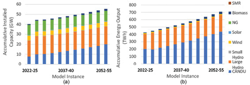
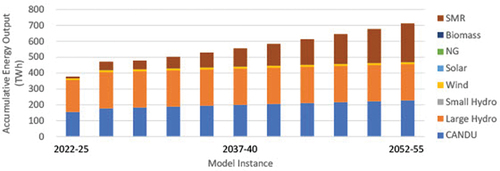
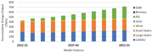
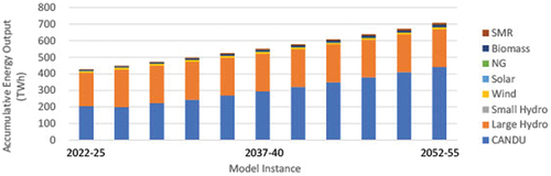
The integration of SMR-based capacities was demonstrated to have a positive impact in every case study of the economically optimized power mix performed in this paper. Figure 3a indicates the optimal combined energy output by all installed utilities in the 2055 power mix using the GE Hitachi–based cost projections for SMR capacity, and Fig. 3b uses the NuScale cost projections. Because of the significant similarities in total projected costs, both candidate SMR designs yielded similar results. In either case, SMR-based energy usage can be seen to grow rapidly across subsequent model instances, demonstrating that despite the requirement to build entirely new capacity in addition to the costs of energy production, SMR usage yields an economic benefit and supplied approximately one-third of the total energy supply throughout the final model instance.

Fig. 3. Optimized 2055 energy mix with (a) GE Hitachi candidate SMR introduction and (b) NuScale iPWR candidate SMR introduction.

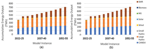
In addition to the growth of electrical power demand over the 33-year modeling period, it should be recognized that the rapid growth in SMR usage is a result of the immediate phaseout of natural gas–based energy output. This is primarily a result of the imposition of the federally mandated carbon tax, which maintains a current value of $50/tonne CO₂ and will continue to rise annually until a final value of $170/tonne CO₂ is achieved, where it will remain constant indefinitely.^[14] The usage of natural gas throughout the model period is heavily constrained by the additional costs of the imposed carbon tax, and this cost increase is directly proportional to its usage. Alternative scenarios that consider a less aggressive, constant-valued carbon tax and a “no carbon tax” case are addressed below in the sensitivity analysis.

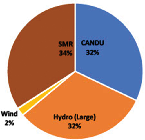
In this optimized scenario, SMR capacity generated an average hourly power output of 9.24 GW in the final model instance of the period for both candidate SMR cases, representing the 2052–2055 power mix. This value is noticeably higher than the corresponding average hourly power outputs of both CANDU and large hydropower, which generated hourly average values of 8.69 and 8.65 GW, respectively. As can be seen in Fig. 4, SMRs have the single greatest contribution to the average hourly load in the optimized 2055 power mix.

Fig. 4. Proportionate contributions to the average hourly load in the final model instance of the optimized scenario.

In addition to SMRs, large hydropower underwent a significant increase in usage from the point of initiation of this model period. Because of the physical limitations regarding the remaining availability of large hydropower potential in Ontario, this utility was heavily constrained by its ceiling value for new capacity installations, as well as its effective capacity factor. The imposed capacity factor for large hydropower was determined by the historical capacity factor values for Ontario’s large hydropower plants, specifically using 2020 and 2021 data from IESO and Ontario Power Generation.^[7,27]

It should be cautiously noted that Ontario currently does not have any large-scale means of storing energy generated by variable renewable plant types such as wind or PV employed.^[28] Such systems may play a vital role in the efficacy of renewable-based and hybrid-based power mixes, increasing both the effective amount of usable energy and the dependability of these plant types. Because of the lack of widespread provincial availability, storage plant types are not considered in this paper, which may have led to a negative biasing on the future potential of wind and PV, as well as their deployment in the optimized power mix. Later analyses will seek to add this technology to consideration once comprehensive data for large-scale Ontario energy storage projects may be obtained.

Despite the reality of intermittency and underwhelming efficiencies making variable renewables undesirable in the optimized scenario, in addition to much of today’s energy market, the ability to store excess energy generated for later use during peak demand times will have an undeniably positive effect on their role in future power mixes and will be considered in later models where applicable. Further, in accordance with the current position of many utilities and policymakers in Ontario today regarding general disinterest in new CANDU installations, the CANDU pricing in the standard SMR optimized scenario utilizes CANDU pricing from a high-cost scenario to limit the model’s CANDU development. Section III.F compares SMRs with more idealized CANDU cost values.

III.B. Optimized Capacity Installations

With the introduction of the aforementioned carbon tax and the national commitment to reduce GHG emissions, the development of new carbon-free capacities is required to meet the growing demand. The IESO’s 2021 APO estimates that in an optimistic scenario in which those resources with expiring contracts will still be 100% available, the Ontario demand will begin to exceed existing resources by the mid-2030s.^[6] Figure 5 shows that in such a scenario, natural gas will be required to close the gap between demand and supply for several years during a period of peak carbon taxing, increasing costs, and moving Ontario away from emission reduction goals.

Fig. 5. IESO’s evaluation of Ontario’s energy adequacy given existing capabilities.^[6]

For this model, a time step of 1 h was chosen to allow for the accurate consideration of variable renewables and their corresponding availability profiles. This was done to ensure that SMRs be effectively compared with all other capacity types in the Ontario power mix. The optimal installations of varying capacities in the Ontario energy mix over the next 33-year period are illustrated in Figs. 6a and 6b. The rapid deployment of SMR capacity totaling nearly 10 GW resulted in an economically optimized 2055 energy mix. In contrast to the 20-year projection shown in the IESO’s 2021 APO above, the steady introduction of approximately 1 GW of SMR capacity every 3 years (or per model instance) resulted in a correspondingly lower total cost (based on the equivalent supply requirements using currently existing capacities) and the effective phaseout of natural gas usage. Across each model instance, the installed SMR capacity is maintaining a capacity factor of 0.95, the proposed value by both candidate designs.

Fig. 6. Optimized 2055 installed capacities with (a) GE Hitachi candidate SMR introduction and (b) NuScale iPWR candidate SMR introduction.

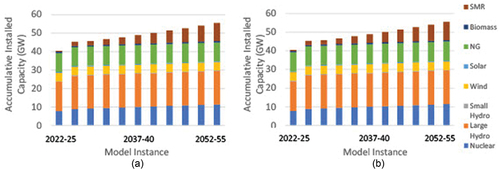
It is important to clarify that the presence of natural gas capacity in the above figures (Figs. 6a and 6b) is entirely a result of the initial, preexisting capacity values set in the first model instance and based on real-world data. As there currently exists no mechanism or purpose for the model to dispose of this capacity, it remains as a static value; however, the model refrains from building additional natural gas capacity or utilizing the existing capacity by any measurable amount in the optimized scenario.

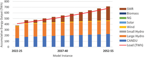
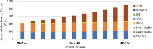
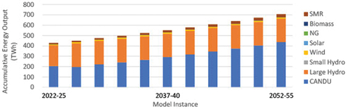
In comparison to the IESO’s projected evaluation of Ontario’s energy adequacy, Figs. 5 and 7 demonstrate the effective increase in accumulative output energy within the optimized scenario in response to the increasing demand (represented by an approximated average demand curve) using the GE Hitachi candidate SMR scenario. This comparison demonstrates the ability of SMRs to bridge the gap displayed in Fig. 5 between Ontario’s supply and the expected demand. The economic viability of SMRs is presented here, being that it was the capacity type selected to meet the demand in an economically optimized scenario. The surplus energy output that is seen in this figure is generated as a surplus constraint in response to assumed losses.

Fig. 7. Evaluation of energy adequacy of Ontario’s accumulative energy output in optimized GE Hitachi SMR scenario.

III.C. Transition to a Net-Zero Power Mix

A significant starting point for the optimized power mix scenario begins with the first model instance and the immediate phaseout of natural gas. The 2030 Emissions Reduction Plan outlines Canada’s goals to achieve a 40% reduction in emissions from 2005 levels by 2030, a significant milestone in the end goal of becoming net zero in 2050.^[28,29]

With the elimination of natural gas, Ontario’s sole remaining GHG emitting utility, the province may become net zero while avoiding additional costs due to the federal carbon tax. As can be seen in Fig. 8, the effect of this shift away from natural gas results in an objective function value (OBJ) that is approximately 7% higher for the first model instance than the resulting trendline from subsequent model instance OBJ values would have suggested. However, this is followed by an immediate reduction in cost during the second model instance, in which the OBJ value is approximately 3% lower than would be expected by the linear trendline. This immediate change is expected as the installed SMR capacity exceeds 2 GW and the first cost reductions from NOAK costs are applied.

Fig. 8. Comparison of the growing average demand alongside the OBJ values for the GE Hitachi and no-SMR optimized scenarios. A trendline is included to compare the GE Hitachi OBJ values with a linear trend.

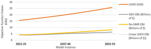
Following these initial two model instances, the subsequent OBJ values begin to follow a far more linear trend. Slight increases and decreases may still be seen, resulting primarily from the loss of CANDU capacity to refurbishments and decommissions (increasing OBJ values), and the reduction in cost as additional NOAK milestones are surpassed (decreasing OBJ values). The rate of increase of the load requirements is significantly higher than that of the OBJ trend in the SMR scenarios, indicating an increasing value of energy output per dollar.

III.D. No-SMR Scenario and CO₂ Emissions

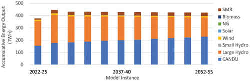
In contrast with the findings of the previous two sections, an investigation was conducted into the cost and resulting power mix in a “no-SMR” scenario. In such a scenario, the model was left to meet the demand requirements of the incrementally increasing load while following all previously mentioned constraints, with the one exception that a new constraint was placed to limit the allowable SMR capacity to zero. The resulting power mix yielded significant increases in the installation amounts of CANDU and biomass capacities (Fig. 9a). CANDU capacity increased by 75%, and biomass capacity increased by 155% compared to their installed capacity values in the previously discussed scenarios.

Fig. 9. Optimized 2055 no-SMR scenario: (a) installed capacity values and (b) accumulative energy output.

When considering the accumulative energy output in the no-SMR scenario, the most notable changes were in the usage of CANDU, biomass, and natural gas utilities (Fig. 9b). Despite the presence of some wind and PV output, the usage of the variable renewables remained largely unchanged. This is likely due to the increased need for both additional baseload support in the absence of SMR capacity (provided by increased CANDU capacity) and additional flexibility in operational output (provided by both natural gas and biomass). The effective capacity factor of CANDU increased from 0.76 in previous scenarios to 0.84 in the final model instance of this scenario. Biomass increased in usage from a negligible energy output to a capacity factor of 0.57 while natural gas was used periodically to reduce stress during times of peak demand (CF < 0.01).

As a result of the required natural gas usage by the no-SMR scenario, the net CO₂ emissions are a nonzero value for the first time. The accumulative natural gas usage over the entire model period was 3.45 TW∙h. Depending on the technology in question, this corresponds to approximately 1.2 to 1.8 × 10⁶ tonnes of CO₂.^[2] The additional cost resulting from these emissions will be discussed in the next section.

III.E. Comparison of Projected Power Generation Costs

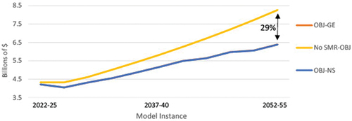
The total cost of power generation is minimized in each model instance through linear optimization of the objective function. The economic viability of SMRs is, thus, tested on the basis of the linear programming model’s preferential selecting and the construction of a power mix that meets the real-world constraints while minimizing the cost. The results discussed above outline the decisions made by the model in favor of significant integration into the Ontario energy mix for two leading SMR candidate designs. The resulting costs of the two SMR candidate designs were very nearly identical in application, with the NuScale iPWR having slightly higher initial costs, but marginally lower fixed and variable O&M costs than the projected costs for GE Hitachi’s BWRX-300.^[21,26] When compared in the final model instance, following the application of expected learning curve cost reductions, the NuScale and GE Hitachi–based power mix scenarios have corresponding OBJ values that vary by less than 1% ($6.38 × 10⁹ versus $6.39 × 10⁹, respectively), as can be seen in Fig. 10. Notably, the major difference in cost occurs between the two SMR-based scenarios and the no-SMR scenario, represented in yellow (Fig. 10). As can be expected given the results of the first two scenarios, constraining the use of SMR capacity to zero had a drastic effect on the cost of the power mix, as the supply now needed to rely on more costly capacity installations and a carbon-emitting utility. The overall effect was a net increase in the observed OBJ value of the final model instance of 29% when compared to either of the candidate SMR-based scenarios.

Fig. 10. Comparison of scenario OBJ values over time. The NuScale (NS) and GE Hitachi (GE) lines are too close to distinguish.

Finally, a scenario was considered in which early investment into SMR-based capacity led to the immediate construction of 2 GW of capacity before the first model instance. The fixed costs of this capacity have still been applied to the OBJ value. The effect of this early investment is to immediately reduce the O&M costs by achieving the first learning curve milestone. Though subtle, the results may be seen in Fig. 11. Following an initial cost increase for the first model instance of the $K_{0,8}=2\mathrm{G}\mathrm{W}$ scenario of 2.07% (due to the inclusion of the SMR construction costs), the OBJ value for the subsequent two model instances quickly reduced for this scenario. The reductions in the OBJ values of the second and third model instances were 1.37% and 1.30%, respectively, yielding a net cost reduction of 0.60%. Following these three model instances, the OBJ values for all remaining model instances were equal.

Fig. 11. Comparison of OBJ values of new GE Hitachi SMR scenario with no starting capacity (blue) and an initial investment of 2 GW into SMR capacity (orange). Agreeable results were found for a NuScale-based scenario.

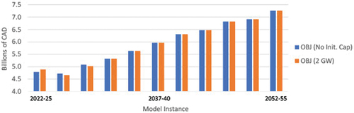
This net cost reduction is seen over the first 9 years (three model instances), after which the subsequent instances maintain equal OBJ values from scenario to scenario. In the case that SMRs are adopted in other countries and project experience is gained globally, the learning curve of production effects on cost reduction would be applied at a significantly faster rate, leading to possible further reductions in up-front costs for the early Canadian SMRs. In addition, it should be noted that these OBJ values have a slightly higher absolute value than those compared in previous sections. This is due to the inclusion of preexisting capacity costs in these two scenarios in order to compare the effect of the early installation of SMR capacity. As a result, the absolute OBJ values of the two scenarios discussed in this section are considered less realistic than the previously discussed scenarios in earlier sections. However, the relative difference between the OBJ values discussed in this section and the corresponding net cost reduction are considered realistic. This is because the additional costs applied to these two scenarios in this section have been done equally; thus, they may be negated when analyzing the relative difference.

III.F. Cost Competitiveness of SMRs Versus CANDUs

Despite significant research into the area of projected SMR costs, the expected values remain highly disputed by third-party analysts and skeptics. This paper investigates the comparison of historical CANDU costs and various SMR costs in order to identify a cost profile for SMRs that would indicate at what point they would become economically competitive with new CANDU projects. Within this model, dynamic cost values were applied in order to approximate the effects of learning curve cost reductions on the introduction of new SMR and CANDU installations.

Figure 12 illustrates several projected FOAK and NOAK cost values for these technologies with approximated curves. In practice, learning curve cost reductions are applied with each doubling of installed capacity until the technology has reached n installed units and is considered a well-established technology, following an asymptotic curve.^[20,30] Generally, this corresponds to an installed capacity value of 10 to 15 GW or a minimum of 34 installed units for a 300-MW(electric) SMR before flattening out.^[20] This paper has assumed a minimum NOAK cost of 60% of the original SMR/CANDU FOAK cost.

Fig. 12. Various projected learning curves corresponding to approximate costs at 0 GW installed (FOAK) and 10 to 16 GW installed (NOAK). For this case, existing CANDU capacity has been ignored.^{[4,5,33,36,37]}

Modern construction costs for new CANDU projects were based on cost projections for two-unit CANDU 6 reactors from Auckland University of Technology and Canadian Energy Research Institute.^[31,32] Because of the significant amount of time that has elapsed since the last domestic CANDU reactor was constructed, it has been considered as a new technology for this scenario and is subject to NOAK cost reductions that have been approximated to follow the observed cost reductions that have resulted from repeated construction of new large reactors in Korea.^[33] The standard version of the model employs SMR cost projections from the Minerals Council of Australia for both SMR candidate designs in the base scenarios.^[21] These values were selected on the grounds that they are recently published projections and can be considered a middle ground for cost projections while being agreeable with other third-party cost projections.^[21] SMR cost projections for Lazard’s 2019 levelized cost of electricity report (FOAK and NOAK) and SMR START are also included in Fig. 11.^[34,35]

The effect of this comparison was to determine the transition point at which the model would opt to develop new SMR capacity in lieu of new CANDU. A wide range of cost values was tested for both categories, and third-party cost projections from relevant reports have been marked on Figs. 13a and 13b (including both FOAK and NOAK projections where possible). Using a constant total variable cost of $5.63/MW∙h for the candidate SMR (comparably similar to CANDU), SMRs gained advantage when the total fixed cost dropped below $8611.45/kW. Conversely, in the case of a constant total fixed cost of $8055.62/kW (taken from recent third-party NuScale cost projections and converted to 2022 Canadian dollars),^[21] SMRs were constructed when the total variable cost reduced below $5.67/MW∙h.

Fig. 13. A comparison of the installed capacity values for SMRs versus CANDU reactors when (a) varying the total variable cost (fuel and variable O&M combined) and (b) varying the total fixed cost (OCC and fixed O&M combined).^{[4,5,33,36,37]}

III.G. Sensitivity Analysis

In order to test the consistency of the model and its dependency on various input values, sensitivity tests were performed for a variety of situations. These tests can be vital as they can expose any areas of oversensitivity within a model and determine the dependency of the results on specific setup parameters. Because of the significant similarity of results between both the GE Hitachi and NuScale candidate SMR design scenarios, only the GE Hitachi results are discussed in the following sections.

III.G.1. Testing of Dependency on Carbon Tax

III.G.1.a. Constant Carbon Tax Value

A sensitivity analysis was performed on the effect of the carbon tax on the optimized SMR scenario. Considering the possibility of rollback on government policy regarding carbon tax, it is important to test how the scenario may change under different carbon constraints. For this test, the carbon constraint was reduced from the expected carbon pricing plan mentioned previously in this paper to a constant carbon price of $50/tonne CO₂. This price value will remain static for the entirety of the model period. This is the carbon price that exists in Canada today and will begin increasing next year under the current plan.

Minimal effects were found as a result of this change (Fig. 14). As the current tax of $50/tonne CO₂ is still considered to be significant cost, this result agrees with expectation and demonstrates that SMRs may remain economically competitive in the event of a carbon tax policy rollback.

Fig. 14. Projected accumulative energy output per model instance in constant CO₂ pricing scenario.

III.G.1.b. Carbon Tax Value of 0

In this scenario, the carbon tax for the model was reduced to a static value of 0. This was done to test the response of the model when the rigid CO₂ pricing constraints were loosened. As should be expected, the reduction in costs against natural gas usage led to a significant rise in the use of this utility due to its very low up-front and O&M costs (Fig. 15). This demonstrates the sensitivity of the model to changes in pricing and allows for consideration of how one might expect the current energy mix to shift if the price of natural gas as a fuel resource were to increase.

Fig. 15. Projected accumulative energy output per model instance in a scenario with no CO₂ pricing.

III.G.2. Testing of Dependency on Load Variations

III.G.2.a. Effects of Rapidly Increasing Load

In this test, the response of the scenario to a rapidly increasing load (increased from 1.7% annual increase to 2.5%) was reviewed (Fig. 16). The resulting scenario behaved as expected, outputting a larger portion of the SMR-based capacity than was previously required in order to supply the demand while optimizing the cost. As new SMR-based capacity was determined to be economically optimal in previous, similarly constrained scenarios, it follows that increasing the demand would increase its usage.

Fig. 16. Accumulative energy output from 2.5% annual increasing demand scenario. As expected, the resulting SMR output increased dramatically.

III.G.2.b. Effects of Static Load

This case was used to test the response of the system to a load array value that remained constant across all model instances (Fig. 17). This was done to determine if in an unexpected situation where the Ontario demand does not increase as significantly as expected, the SMR-based capacity will still be utilized by the model. Because of the presence of the carbon tax, the model performed as expected by phasing out costly natural gas usage and installing a minimal amount of SMR capacity to meet the demand and constraints sufficiently. Slight output variations may be seen in the first four model instances due to varying CANDU capacity values (see Sec. II.B.3).

Fig. 17. Accumulative energy output from static load scenario. Without the increasing demand, it follows that SMR usage should be reduced overall, acting only to replace more expensive plant types.

III.G.3. Testing of Dependency on Fixed and Variable Costs

Finally, the response of the system to price increases was tested in this scenario. The fixed and variable costs for SMR-based capacity have been increased by 100%, with the resulting mix of outputs seen in Fig. 18. As expected, with the dramatic increase in cost of SMRs, this plant type is no longer considered economically competitive by the model and, thus, has not been used impactfully in the scenario.

Fig. 18. Projected accumulative energy output from high SMR cost scenario (100% increase). With the significant increase in associated costs, SMRs are no longer effective in the economically optimized model.

Additionally, the increased cost scenario was again run with a cost increase of only 50%. The purpose of this additional test was to review the model’s sensitivity to an incremental, more realistic change in costs. The energy output values from this scenario (Fig. 19) again aligned with expectations, as the SMR output increased incrementally, reaching a total 3-year energy output of approximately 31 TW∙h for the final model instance with 1.23 GW of installed capacity (no applied learning curve cost reductions). This demonstrates that with a cost increase of 50% to both fixed and variable costs, SMR-based capacity is still economically viable in the optimized power mix, though to a lesser extent compared to normally priced scenarios.

Fig. 19. Projected accumulative energy output from 50% SMR cost increase scenario. SMR usage has dropped significantly in lieu of CANDU use, though it is still viable to a small degree.

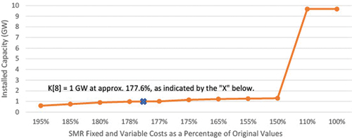
This sensitivity analysis may also be applied with a higher degree of precision in order to approximate the tipping point of the total SMR cost, identifying at what threshold value they will become economically viable. The total cost of SMRs from the optimized scenario has been incrementally decreased and remodeled using the same methodology as above to determine the cost value at which SMRs begin to have an impactful presence within the optimized future power mix. For the purpose of this test, an “impactful presence” has been arbitrarily determined to be a threshold value of 1-GW installed capacity in the optimized scenario due to the asymptotic nature of the modeling outputs near boundary conditions. As can be seen in Fig. 20, the tipping point in this analysis occurs at a fixed cost of $364.88/kW and a variable cost of $2.13/kW∙h (which is a 77.76% increase from the projected values used in the optimized scenario). As the purpose is to test the threshold value for the FOAK costs, learning curve cost reductions have been applied for the purpose of this analysis.

Fig. 20. Sensitivity analysis of the effect of varying fixed and variable SMR cost values on installed SMR capacity. Costs are represented as a fractional percentage of the original fixed and variable costs used in the optimized scenario, and the installed SMR capacity surpassed 1 GW at 177.6%, or a 77.6% increase from the original values.

IV. CONCLUSION AND FUTURE IMPLICATIONS

This paper evaluates the long-term viability of SMR deployment into the existing Ontario power mix over a 33-year period by investigating the 2055 economically optimized power mix. A semidynamic method was used in which a static model solved a series of model instances using linear optimization. Flow Control processes were introduced that allowed the sharing of data between statically solved model instances via postprocessing, applying a temporal element to the analysis. Using the postprocessing capabilities, the model instances were iterated through a larger time period, establishing the semidynamic approach. With this method, dynamic factors such as forecasted demand growth, increasing capacity installations, learning curve applications, and reactor refurbishment and decommissioning schedules were applied to the modeling scenarios. Such an analysis is useful in planning for future energy supply growth to match demand while minimizing spending, ensuring the reduction of CO₂ emissions, and preparing for the magnitude of new capacity types. In the case of SMR-based capacity, estimates of Ontario’s future dependence on this utility in a variety of scenarios not only will aid in government planning but also will provide significant secondary benefits to groups such as the Nuclear Waste Management Organization of Canada that require accurate projections for waste generation from current and future nuclear projects.

Results from the generated scenarios presented above show that in the case of the two candidate SMR reactor designs considered, SMR-based capacity is an economically viable method of power generation that can also aid greatly in the shift to net-zero emissions. When introduced to the existing Ontario energy mix, SMRs were immediately employed by the model to begin phasing out natural gas under today’s applied carbon tax and could compete with already-installed utilities, despite having to undergo both installation and operation costs. Following the increase in load demands throughout the model period, SMR installed capacity experienced the single large rate of capacity growth between model instances. Further, following the completion of the final model instance and the 33-year period, SMRs were the primary contributor of energy output in the 2055 economically optimized power mix (34% SMR, 32% CANDU, 31.9% large hydropower, 2% wind, and 0.1% PV). Despite having 0 GW of installed capacity at the start of the model period, the final 2055 optimized power mix contained approximately 9.73 GW of installed SMR capacity in both design scenarios.

Next, a comparison was done between the above results and the no-SMR scenario, in which Ontario’s 2055 economically optimized power mix is modeled under currently pricing projections and SMR usage is heavily constrained to zero. The results found a significant increase in the total cost of the resulting power mix in the final model instance (net OBJ increase of 29%). Additionally, the dependence of the power mix on natural gas usage in the no-SMR scenario increased dramatically, from zero usage to an accumulative energy output of 3.45 TW∙h over the model period. This result is in stark contrast with Ontario’s net-zero emissions goals.

When analyzing the effects of SMR installations on power mix costs, the SMR-based scenarios showed clear reductions for both candidate SMRs that were considered. Upon further review, a scenario was examined in which proactive investing into SMR capacity led to the construction of 2 GW of capacity at the start of the model period. While the entirety of the expected costs was applied to the construction of this capacity, early investment allowed for the learning curve cost reductions to be applied earlier, reducing the overall costs of subsequent operation and further construction. The effect led to a cost reduction of approximately $20 million over the first 9 years (all subsequent OBJ values were equal between the two scenarios).

Finally, sensitivity testing of the model was conducted in order to view its behavior under unexpected conditions and investigate the boundaries of SMR capacity’s viability. As expected, scenarios in which the carbon tax was reduced to a constant value remained in favor of SMR deployment while no-carbon tax or emission limit scenarios saw the results change significantly in favor of natural gas. In the case of variability in the future demand growth, SMRs were still favored over natural gas and other utility types, but SMR installation was limited to meet the reduced demand in order to optimize costs. Finally, increases in the expected SMR costs (and no learning curve reductions) lead to expected reductions in the rate of installation and usage. In the case of major cost increase (100% increase), SMR deployment was largely minimized in favor of other utilities (400 MW installed). With a more realistic cost increase of 50%, SMR deployment was reduced from initial scenarios but still maintained a final installation value of 1.23 GW.

Future work consists of increasing the complexity of the model to include a better analysis of the nuclear fuel cycle (comprehensive fuel pricing, waste management); modern energy storage systems for variable renewables; detailed transmission cost considerations, particularly for utilities located in rural areas; advancements in natural gas technology such as carbon capture and sequestration; rapid demand expansions from causes such as electric car deployment; and a comprehensive analysis of expected SMR designs, maximum rates of construction, and considerations for specific unit capacities.

Acknowledgments

The authors would like to thank the Japanese Society for the Promotion of Science, in addition to Fujii-Komiyama Laboratory at the University of Tokyo, and Mitacs Globalink for the joint fellowship opportunity that aided in supporting this research.

Disclosure Statement

No potential conflict of interest was reported by the author(s).

Notes

^a In standard practice, Ontario is considered to have these six resources; for the purpose of this study, however, large and small hydropower has been separated into two unique resources due to their significant differences in cost.

APPENDIX

A.I. FLOW CONTROL OUTLINE

Flow Control refers to a process within CPLEX that allows a specified number of iterations (or model instances) to be generated and solved in sequence. This function allows for the addition of temporal considerations through the combination of iterative solving and inter-instance data manipulation. With the addition of a .main file to an existing model, which would normally comprise model (.mod) and data (.dat) files, the user may now set CPLEX to run a specified number of solves while applying postprocessing data edits between subsequent iterations. The result is a semidynamic model, as subsequent model instances can now be generated with updated input data from the previous solve and yield a more informed end result based on a series of static solutions at specified time-step intervals between $t=0$ and $t=t_{final}$. The model used in this investigation generates 11 instances, each representing a 3-year period with hourly time steps (26 280 h). As the postprocessing allows for output data to be passed from one solved instance to the subsequent one, the result is a semicontinuous 33-year analysis yielding a theoretically more accurate scenario for the optimized 2055 Ontario power mix.

A.II. ADDITIONAL INPUT VALUES

Table A.I provides additional input values.

TABLE A.I Input Values for Model Constants

K0,1’	7778 MW	Installed CANDU capacity variations over time
K0,1”	8889 MW
K0,1”’	9172 MW
K0,1””	9989 MW
σ	0.04%	Average expected transmission losses
ζ	1.05%	Projected demand increase per model instance
${\phi }_{max,j},$${\phi }_{min,j}$	j = 1 0.95, 0.76	Minimum and maximum output power levels, respectively, for j’th power plant
	j = 2 1, 0
	j = 3 1, 0
	j = 4 1, 0^a
	j = 5 1, 0^a
	j = 6 1, 0
	j = 7 1, 0
	j = 8 1, 0.40
δI,j, δD,j	j = 1 0.60, 0.60	Maximum increase and decrease rate of changes of power outputs for j’th power plant, respectively
	j = 2 0.05, 0.05
	j = 3 0.05, 0.05
	j = 4 1, 0^a
	j = 5 1, 0^a
	j = 6 0.82, 0.75
	j = 7 0.31, 0.58
	j = 8 0.60, 0.60
λ	0.864	Effective CANDU capacity reducing factor
Ωn, n = 1	2 GW	Milestone capacity values for application of NOAK cost reductions to SMR installed capacity
Ωn, n = 2	4 GW
Ωn, n = 3	6 GW
Ωn, n = 4	8 GW
α	12%	NOAK coefficient for cost reductions

^aThe minimum/maximum values for j = 4, 5 (wind, PV) are determined by their availability profiles.

References

- “A Call to Action: A Canadian Roadmap for Small Modular Reactors,” Canadian Small Modular Reactor Roadmap Steering Committee (2018).
- NUCLEAR POWER TECHNOLOGY DEVELOPMENT SECTION, “Status of Advanced Light Water Reactor Designs,” International Atomic Energy Agency (May 2004); https://www-pub.iaea.org/MTCD/Publications/PDF/te_1391_web.pdf (current as of May 20, 2022).
- Small Modular Reactors: Can Building Nuclear Power Become More Cost-Effective? Ernst & Young LLP, London (2016).
- B. HEARD, “SMRs: Small Modular Reactors in the Australian Context,” Minerals Council of Australia (2021).
- “Annual Planning Outlook, Ontario’s Electricity System Needs: 2023-2042,” Independent Electricity System Operator (2021).
- “Ontario’s Supply Mix,” Independent Electricity System Operator (Oct. 2020); https://www.ieso.ca/en/Learn/Ontario-Supply-Mix/Ontario-Energy-Capacity (current as of May 5, 2020).
- S. I. GASS, Linear Programming Methods and Applications, 5th ed., Dover Publications, Mineola, New York (1995).
- G. DOLUWEERA and et al., “A Comprehensive Guide to Electricity Generation Options in Canada,” Canadian Energy Research Institute (2018).
- M. AYRES, M. MORGAN, and M. STOGRAN, “Levelized Unit Electricity Cost Comparison of Alternate Technologies for Baseload Generation in Ontario,” Canadian Energy Research Institute (2004).
- R. KOMIYAMA and Y. FUJII, “Long-Term Scenario Analysis of Nuclear Energy and Variable Renewables in Japan’s Power Generation Mix Considering Flexible Power Resources,” Energy Policy, 83, 169 (2015); https://doi.org/10.1016/j.enpol.2015.04.005.
- “2030 Emissions Reduction Plan: Clean Air, Strong Economy,” Government of Canada (July 12, 2022); https://www.canada.ca/en/services/environment/weather/climatechange/climate-plan/climate-plan-overview/emissions-reduction-2030.html (current as of May 20, 2022).
- “Greenhouse Gas Pollution Pricing Act: Annual Report for 2020,” Government of Canada (2020).
- “Power Data,” Independent Electricity System Operator ( Jan. 2021); https://www.ieso.ca/en/Power-Data (current as of May 2021).
- M. MCCLEARN, “Ontario Eyes Hydroelectric Projects as Demand for Power Rises,” The Globe and Mail (Jan. 23, 2022).
- D. B. RICHARDSON and D. HARVEY, “Optimizing Renewable Energy, Demand Response and Energy Storage to Replace Conventional Fuels in Ontario, Canada,” Energy, 93, 1447 (2015).
- “Data Directory,” Independent Electricity System Operator (2022); https://www.ieso.ca/en/Power-Data/Data-Directory (current as of Jan. 25, 2022).
- S. PFENNINGER, “Renewables Ninja,” Grantham Institute at Imperial College London (2022); Renewables.ninja (current as of Sep. 2021).
- L. POURET and W. NUTTALL, “Can Nuclear Power Be Flexible?” Energy Policy Research Group, Cambridge Judge Business School (2007).
- Z. LIU and J. FAN, “Technical Readiness Assessment of Small Modular Reactor (SMR) Designs,” Prog. Nucl. Energy, 70, 20 (2014); https://doi.org/10.1016/j.pnucene.2013.07.005.
- “Guide to Operating Reserve,” Independent Electricity System Operator (2011).
- J. M. HOPWOOD, M. SOULARD, and R. LALONDE, “Advanced CANDU Reactor Design for Operability,” Proc. Int. Conf. Global Environment and Advanced Nuclear Power Plants (GENES4/ANP2003), Kyoto, Japan, September 15–19, 2003.
- N. ARKALGUD and S. RUX, “Examples of Flow Control in OPL,” WebSphere® Support Technical Exchange (2013).
- “Annual Planning Outlook, A View of Ontario’s Electricity System Needs,” Independent Electricity System Operator (2019).
- “Annual Planning Outlook, Ontario’s Electricity System Needs: 2022–2040,” Independent Electricity System Operator (2020).
- B. VEGEL and J. C. QUINN, “Economic Evaluation of Small Modular Nuclear Reactors and the Complications of Regulatory Fee Structures,” Energy Policy, 104C, 395 (2017).
- “Achieving Balance—Ontario’s Long-Term Energy Plan,” Ministry of Energy, Toronto (2013).
- “Nuclear Refurbishment: An Assesment of the Financial Risks of the Nuclear Refurbishment Plan,” Financial Accountability Office of Ontario (2017).
- “Pre-Licensing Vendor Design Review,” Canadian Nuclear Safety Commission (Jan. 26, 2022); https://nuclearsafety.gc.ca/eng/reactors/power-plants/pre-licensing-vendor-design-review/ (current as of May 25, 2022).
- “Nuscale’s Affordable SMR Technology for All,” NuScale Power LLC (Mar. 2020); https://www.nuscalepower.com/newsletter/nucleus-spring-2020/featured-topic-cost-competitive (current as of May 20, 2021).
- “Hydroelectric Power,” Ontario Power Generation (2022); https://www.opg.com/powering-ontario/our-generation/hydro/ (current as of May 20, 2022).
- “By the Numbers,” Canadian Renewable Energy Association (Dec. 31, 2021); https://renewablesassociation.ca/by-the-numbers/ (current as of May 2022).
- K.-H. MOON and S.-S. KIM, “An Exploratory Study on a Target Capital Cost and Cost Reduction Methodologies of Innovative SMR in Korea,” Transactions of the Korean Nuclear Society Virtual Spring Meeting, 2020.
- B. WILSON, “Nuclear Feasibility for a New Zealand System,” Auckland University of Technology (2009).
- “Nuclear Power in South Korea,” World Nuclear Association (June 2022); https://world-nuclear.org/information-library/country-profiles/countries-o-s/south-korea.aspx (current as of Sep. 10, 2022).
- A. FLETCHER, “Can NuScale’s SMR Compete with Natural Gas?” The Breakthrough Institute (Sep. 8, 2020).
- “The Economics of Small Modular Reactors,” SMR Start (2017).
- CANTEACH, “The Conventional Side of the Station,” CANDU Fundamentals, p. 261, Ontario Power Generation.