Implementing Component Degradations into a Modelica Model of an iPWR System to Develop Health Monitoring Techniques

Abstract

The economic operation of small modular reactors will partly rely on managing and reducing inspection and maintenance activities while supporting new operational paradigms like load-following. Turbine control valves throttle the steam from the steam generator into the steam turbine while maintaining the pressure within the steam generator at a constant set point. Degradation of these components could impact the ability to manage electrical power production.

Utilizing the Idaho National Laboratory Hybrid repository and the Oak Ridge National Laboratory TRANSFORM library developed for multiphysics simulations in Dymola/Modelica, an integral pressurized water reactor system was modeled based on the available specifications of the NuScale power module. The effects of various component degradation modes have been implemented into the model in order to simulate faulted plant data during both steady-state and load-following operations. The fault modes resemble different physical fault modes that may occur at an operating nuclear power plant; a leaking turbine control valve and a valve actuator failure due to loss of hydraulic pressure have been implemented.

A neural network autoencoder is employed in conjunction with statistical analysis, namely, simple signal thresholding (SST) or sequential probability ratio testing (SPRT), to identify the presence of a fault. Fuzzy logic is additionally employed in a novel and promising manner to classify the state of the system based on the cumulative sum of the neural network residuals. SST and SPRT are both successfully validated using healthy data and proved capable of identifying both fault types; fuzzy logic identified the false positives and classified the faulted data correctly.

Keywords:

• Degradation modeling
• turbine control valve
• integral pressurized water reactor
• anomaly detection
• fuzzy logic classification

I. INTRODUCTION

The economic operation of small modular reactors (SMRs) will partly rely on managing and reducing inspection and maintenance activities while supporting new operational paradigms like load-following (LF). It is imperative for SMRs to have the ability to load-follow in tandem with variable energy sources, such as wind and solar, to meet the demand of the energy grid.^[1] An overall goal of SMRs is to make nuclear energy more economically attractive, while simplifying the construction and manufacturing processes and retaining the impressive safety record of commercial nuclear power plants (NPPs).

Operating costs can be reduced by limiting component maintenance frequency, which could be justified by online health monitoring techniques. The health and performance of components would be trackable in real time by the plant operators and engineers, allowing for efficient and economic operation of a multi-unit site.^[2] Historically, it has been standard in the nuclear power industry to perform maintenance on a schedule. Alternatively, condition-based maintenance could justify fewer maintenance activities without compromising safety.^[3]

This work explores methods that promote the economic operation of SMRs by partially enabling condition-based maintenance, effectively lowering operation and maintenance costs. Techniques developed in this work could be used in real time to monitor the state of an operating reactor, identify the presence of a fault, and classify which fault mode is present. This is a flexible framework that could be applied to various nuclear reactor types. In this work, simulation data of an integral pressurized water reactor (iPWR) is used to perform anomaly detection of various fault modes in the turbine control valve (TCV) system.

The iPWR model is based on available information for the NuScale power module (NPM).^[4] The NPM consists of a singular vessel containing the reactor core, pressurizer, and steam generator (SG), and a complete balance-of-plant (BOP), including the steam turbine, condenser, feedwater pump (FWP) and valve, etc. An advantage of the iPWR design philosophy is the decreased probability of a loss-of-coolant accident. Integrating major components and utilizing natural convection to cool the reactor core results in fewer engineered components. However, the compact and self-contained nature of iPWRs may make maintenance and inspection activities more challenging to perform.

Steam is generated inside the reactor module within two helical coil, once-through SGs; this steam flows to the BOP, where it is throttled by three valves before entering the high- and low-pressure turbines. TCVs throttle the steam from the SG into the steam turbine while maintaining the pressure within the SG at a constant set point. Following the condensation of the steam, water is fed back into the SG via the FWP.^[4] Degradation of any of these components could impact the ability to manage electrical power production. This research focuses on potential degradation modes in the BOP components. Further, we consider fault modes and fault magnitudes that may impact the performance of the iPWR in terms of its flexibility and ability to meet power demands, but would not impact plant safety.

Utilizing the Idaho National Laboratory (INL) Hybrid repository^[5] and the Oak Ridge National Laboratory (ORNL) Transient Simulation Framework of Reconfigurable Modules (TRANSFORM) library^[6] developed for Dymola/Modelica, the NPM has been modeled. Dymola is a modeling and simulation software graphical user interface based on Modelica, which is an object-oriented, multidomain coding language. TRANSFORM was made for use in the Dymola modeling environment. The NPM was replicated and validated for both steady-state (SS) and LF operation.^[7]

Further, the effects of degraded components have been modeled in Dymola to generate data from an “unhealthy” or “faulted” system. In order to make the simulation data better resemble plant data, random variation was added. Noise was added such that the shape and trend of the data were unaffected, but a resemblance of instrumentation noise is present. The TCV controller is the only variable void of any noise due to the nature of its output.

This paper presents the simulation and detection of two TCV fault modes in an iPWR. Section II describes the system model implemented in the Modelica modeling language. Section III provides more details about the simulation of the two TCV fault modes: steam leakage and hydraulic pressure loss. The fault detection methodologies investigated, namely, autoencoder-based error correction and residual analysis, are described in Sec. IV. Fuzzy logic has been employed on top of traditional fault detection in order to identify false-fault predictions and differentiate the fault modes; this process is described in Sec. V. Finally, Sec. VI presents the results of applying these methods, and Sec. VII summarizes the current study and highlights areas for future development.

II. iPWR AND BOP MODEL

A multiphysics model was developed in order to generate the data necessary to perform the operational and diagnostic tasks that define the overall goal of our project. The iPWR was modeled after the NPM and adapted from the INL SMR Dymola package (Hybrid Nuclear Energy Systems Dymola library).^[5] We only modeled one NPM, although the NuScale VOYGR plant would consist of 4, 6, or 12 NPMs. The NPMs at a multimodule site operate independently with dedicated BOP systems, so the work developed here could be extended to multiple instances of a NPM at a single site to support site-wide optimization.

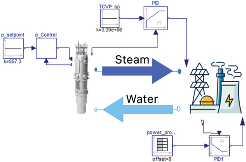
Our NPM model consisted of iPWR and BOP models that were connected through flow and control signals. The most zoomed out view of the model is shown in Fig. 1. A general control strategy was implemented in this model where the feedwater flow rate was linked to the demanded power production through a programmed (open-loop) control. The TCV position is controlled through proportional-integral-derivative (PID) control to maintain a constant steam pressure at the SG outlet. The control rod position, modeled as external reactivity in the point reactor kinetics equations, is controlled by a PID controller to maintain the average coolant temperature across the core. The model did not include turbine bypass, which has been studied in other work (e.g., Ref. [8]). In this work, we relied on power maneuvers in the reactor to adjust energy production in a turbine-leading/reactor-following configuration.

Fig. 1. NPM in the Dymola environment.

The simulation model has been validated against the design parameters given in the NuScale design certification application (DCA).^[4] The validation results are summarized in Ref. [7]. The PID controller gains were selected through an iterative evaluation of controller response to produce the desired response time and overshoot.

III. DEGRADATION MODES

The effects of various degradation modes have been modeled and implemented into the TCV system, which is comprised of the valves and actuators. For the NPM, the TCVs are part of the turbine generator system and follow the main steam isolation valves; they throttle the steam created in the SG into the steam turbine.^[4] These hydraulically actuated, globe-type valves are actuated during power maneuvers to maintain the pressure within the SG during plant operation. Long-term operation of these TCVs may result in wear and degradation; with certain degradation modes, the time until failure may accelerate with increasing actuator movement.

Globe valves have a spherical body and are internally split in two via a horizontal baffle; when the valve is closed, the actuator presses the plug into the seat, which is attached to the baffle. To open and allow greater flow through the valve, the actuator moves the valve stem away from the plug (see Fig. 2). The valve packing seals the stem, avoiding external steam leakage.

Fig. 2. Diagram of a simplified globe valve and hydraulic actuator.

When evaluating failure modes for globe valves, which are widely used for safety and BOP systems in NPPs, the age-based failures are as follows: failure to open, failure to close, plugged valve (limited or no flow through a normally open valve), reverse (internal) leakage, and external leakage.^[9] We are interested in the degradation modes that occur over long timeframes. The most relevant degradation responses for our investigations were the plugged and externally leaking valves. The effect of a plugged valve may be similar to a loss in hydraulic pressure in the actuator, as there is a limitation in the maximum amount of flow through a normally open valve.

The gap between the valve stem and packing is vital to the operation of the control valve. If the gap is too small, the thrust needed by the actuator will be prohibitively large. Alternatively, excess steam leakage will result from a large gap. The stem/packing clearance is typically less than a 0.02-in. (0.5-mm) diametral.^[10] This gap will shrink as the stem or packing oxidizes, which may occur as a result of contact with high-temperature steam. The oxide scales within this gap increase the frictional forces that the actuator must overcome to adjust the valve position.

The stem and packing mechanism can also degrade through normal wear as the valve actuates. As the valve stem moves, friction will cause some degree of wear on the packing material. This natural and expected degradation can be accelerated by increasing the frequency of opening and closing the valve.^[11] If the valve stem is oscillated in one region of the valve stroke, that region may experience localized wear.^[10] Wear will lead to external leakage and lower the thrust necessary for the actuator to overcome friction, potentially leading to over actuation of the valve.

The globe valves in the NuScale design are hydraulically actuated, meaning the movement of the valve stem is dependent on a hydraulic actuation system. It is possible for this system to degrade or fail. Although the NuScale DCA does not provide information on the specifics of the hydraulic actuation system, it may be assumed that the hydraulic oil pressure pushes against the spring and transfers linear momentum to the actuator.^[12] In the case that hydraulic pressure is insufficient for any reason, the valve will resort to a closed position.

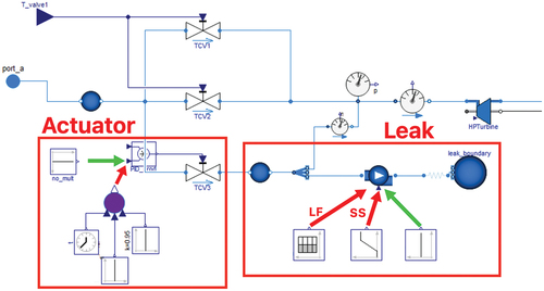
Integrating the physics of degradation into a Modelica model of the TCV directly is not necessary to generate the data needed for this analysis. Instead, the overall effect of degradation is modeled according to the impact on component or system performance. Two independent, physically inspired degradation modes were implemented in our BOP model: an externally leaking TCV and an actuator losing hydraulic pressure. These fault modes can be seen in Fig. 3, labeled “Actuator” and “Leak.” The same Dymola model was used for the generation of both healthy and degraded data. The inputs marked with a green arrow were used when that portion of the TCV was healthy. For the actuator, the same input was used for both LF and SS operations. However there were different inputs for modeling the TCV leak, which are labeled LF and SS, respectively.

Fig. 3. Degradation models within the BOP model in Dymola.

III.A. TCV Leak

Over long time periods, the wear between the TCV stem and packing can lead to an increased gap, which in turn allows steam to leak from the system. To simulate an external steam leak, the steam is routed from the valve to a generic volume with a multiport fitting. The majority of the steam then continues to the rest of the BOP, while a small portion is treated as “leaking steam.” The leaking steam is diverted to a standard pump, then a nominal loss model, and finally an infinite void (boundary condition). The leaking mass flow rate is controlled via an input on the pump. This model can be seen in Fig. 3.

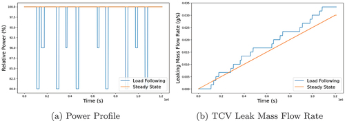
In an operational NPP, the wear on the TCV stem/packing may be accelerated by an increased amount of actuation. This was modeled by increasing the leaking steam mass flow rate every time the power level changed with a corresponding change in TCV position. Over the 2-week LF simulation, there were 20 power changes, and the leak increased incrementally to $0.0333\mathrm{g}/\mathrm{s}$ from 0. To simulate the leak during SS operation, there was a linear increase to $0.03\mathrm{g}/\mathrm{s}$ over the 2-week period. The severity of the SS leak was chosen such that it was around the same magnitude as the LF leak, but not as severe as the more physically motivated LF leak. Figure 4 shows the SS and LF power profiles (Fig. 4a) as well as the rate of leaking steam (Fig. 4b).

Fig. 4. Power profile and leaking mass flow rate.

III.B. Actuator Degradation

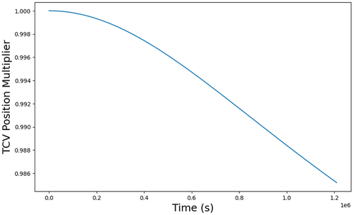
In the implemented control strategy, the TCV position was specified by a PID controller in order to keep the SG pressure at its set point. To simulate a loss in hydraulic pressure within the valve actuator, a mathematical function was created and implemented between the PID controller and TCV position input. This function limited the ability of the valve to become completely open by generating a multiplication factor for the output of the PID controller. Over time, this multiplication factor decreased, further limiting the maximum openness of the valve. During operational transients, the valve can be closed and partially opened to perform the power maneuver.

Equation (1)(1) $\mathit{mul}{t}_{\mathit{factor}}=\mathit{mi}{n}_{\mathit{val}}+\frac{1-\mathit{mi}{\mathit{n}}_{\mathit{val}}}{\sqrt{1+{(\mathit{t}/{\mathit{t}}_{\mathit{step}})}^2}}.$(1) shows the TCV position multiplier $\mathit{mul}{t}_{\mathit{factor}}$, where min_val and t_step define the behavior of the function,

(1) $\mathit{mul}{t}_{\mathit{factor}}=\mathit{mi}{n}_{\mathit{val}}+\frac{1-\mathit{mi}{\mathit{n}}_{\mathit{val}}}{\sqrt{1+{(\mathit{t}/{\mathit{t}}_{\mathit{step}})}^2}}.$(1)

As t approaches infinity, the multiplier goes to min_val. The time of this transition is dictated by t_step.

Some trouble was encountered when attempting to define the physical degradation that would lead to this behavior. When considering the SS results, it could be assumed that the pressure of the actuating oil was continuously decreasing. This would explain the slow decrease in TCV openness. This description for the degradation mechanism becomes problematic when considering LF scenarios. If it were the actuator’s inability to create sufficient thrust to keep the valve open at the correct position, the actuator would not be able to reopen the valve following a power maneuver. As mentioned in Sec. III, this behavior may also resemble a plugged valve, due to the limitation of the flow through the valve.

The parameters used within Eq. (1)(1) $\mathit{mul}{t}_{\mathit{factor}}=\mathit{mi}{n}_{\mathit{val}}+\frac{1-\mathit{mi}{\mathit{n}}_{\mathit{val}}}{\sqrt{1+{(\mathit{t}/{\mathit{t}}_{\mathit{step}})}^2}}.$(1) for our investigation were as follows: min_val = 0.95 and t_step = 1.2 × 10⁶ s. The resulting multiplication factor is shown for the duration of the simulation in Fig. 5.

Fig. 5. Multiplication factor for actuator degradation.

III.C. Data Extraction

Because both degradation modes affect the same component in the BOP, we selected variables that would be able to detect both faults. The iPWR model has hundreds of variables to select from. Here, we focused on variables that would be reasonably measurable in an operating iPWR power plant. Following the extraction of these data from simulations under both LF and SS conditions, random white noise was added to simulate measurement and electronic noise and make the data more realistic for the machine learning section of this project. Ultimately, nine variables were selected:

1. high-pressure turbine output (W)

2. low-pressure turbine output (W)

3. TCV controller response (unitless fraction between 0 and 1)

4. TCV pressure (bar)

5. condenser mass (kg)

6. TCV mass flow rates (one for each of the three TCVs) (kg/s)

7. SG pressure (bar).

Each simulation occurred over 2 weeks, generating 12 000 data points for our analysis. A notional simulation length and LF power profile were used for computational efficiency, solely to indicate when the reactor was not operating in SS. Degradations were implemented on an accelerated timeline for the same reasons. These assumptions are believed to have not affected the validity of the fault detection and classification methodology presented or its ability to detect and classify faults in both LF and SS operational modes.

IV. FAULT DETECTION METHODOLOGY

Previous work on this project explored anomaly detection methods to detect FWP degradation.^[7,13] In that work, three error-correction algorithms were explored: principal component analysis (PCA), auto-associative kernel regression (AAKR), and a neural network (NN) autoencoder. PCA proved to be incapable of capturing the nonlinearities inherent to LF data and was not considered further for this purpose. Both the AAKR and NN autoencoder were able to distinguish between healthy and nonhealthy data in both LF and SS operations.^[7]

A review and analysis of deep learning–based time-series anomaly detection methods is provided in Ref. [14]. The authors praised its data-driven nature and ability to detect faults without extensive domain knowledge. Demonstrations of NN autoencoders exist for various industries with different uses and NN configurations (feedforward, long short-term memory, convolution, and recurrent NNs). Examples of these can be found in Ref. [14] and are demonstrated in Refs. [15–17]. The demonstration in Ref. [17] tested a large variety of machine learning algorithms and found autoencoders to be relatively fast in their training and running times.

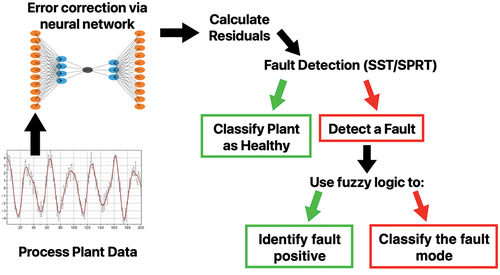
The primary contribution to the state of the art presented here is the application of the NN autoencoder fault detection approach to a SMR operating in both LF and SS modes, as well as a novel use of fuzzy logic for fault classification and verification. The flow diagram in Fig. 6 details this methodology. This section details how processed plant data flow through an autoencoder for error correction, and how fault detection is performed through statistical analysis. If our statistics believe a fault is present, fuzzy logic is applied in order to limit fault positives (by identifying data as healthy) or to classify which fault mode is present. Fuzzy logic classification is described in greater detail in the following section.

Fig. 6. Flow diagram of the fault detection and classification algorithm.

This paper focuses on an autoencoder for error correction and two residual analysis routines for anomaly detection. An autoencoder was constructed in Python using the Keras application programming interface and trained using simulation data containing both LF and SS operations. Autoencoders consist of an encoder and a decoder. The encoder generates a lower-dimensional representation of the input data, while the decoder decompresses the reduced dimensionality to produce an error-corrected version of the inputs. The encoder and decoder are connected through a bottleneck layer that defines the dimensionality of the compressed representation. The error-corrected output of the autoencoder is compared to the measured data (the input) to produce a residual between the two. With this residual, we were able to perform anomaly detection. In this work, we investigated simple signal thresholding (SST) and the sequential probability ratio test (SPRT).

Simple signal thresholding evaluates the NN residuals to determine if any have crossed a predefined threshold that indicates an anomaly. The threshold is typically determined based on the expected residuals under healthy operation to give an acceptable false positive rate. For instance, if a 95% threshold of nominal residuals is used, then 5 out of every 100 healthy observations would be expected to cause an alarm. The threshold used was defined in terms of the standard deviation of each variable’s test residual (the difference between the decoder’s output and the validation data). Utilizing four times the standard deviation for each variable produced acceptable false alarm and true alarm rates.

The SPRT is a statistical hypothesis test that determines if a series of data is more likely from a normal or faulted distribution.^[18] SPRT relies on a stream of residuals to build evidence of an anomaly, unlike SST, which only evaluates individual observations in isolation. This allows SPRT to more quickly detect anomalies and to detect anomalies of smaller magnitude. The threshold used for each variable in the SPRT analysis was dependent on the standard deviation of each variable’s test residual; optimized results were achieved using eight times each standard deviation.

V. FUZZY LOGIC CLASSIFICATION

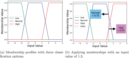
In order to provide a verification of the aforementioned fault detection methodology and to classify the status of the system, fuzzy logic was implemented. This type of logical computing is distinguished by a soft classification style, rather than a binary approach.^[19] Our fuzzy logic looked at the cumulative sum of the NN residuals over the past 1000 data points (about 27.8 h of data), and applied a membership to each variable. For example, when the cumulative sum of the TCV controller response residual over the last 2 days was between −1 and 1, it was classified as normal, otherwise it was (fully or partially) classified as high or low. This process is illustrated in Fig. 7. In this example, the membership functions are shown in Fig. 7a and applied in Fig. 7b. An input value of 1.3 was applied, giving a membership value of 0.7 to the normal classification, 0.3 to high, and 0.0 to low.

Fig. 7. Membership example.

The benefit and purpose of our fuzzy logic classification system were to provide additional analysis of the system, using the trends of the time series data and prior knowledge of the fault modes. Following a fault prediction from SST or SPRT, fuzzy logic was called in order to confirm the presence of a fault (reduce false positives) and identify which fault was provided. In practice, this additional information would allow reactor operators and plant management to improve decision making in regard to plant safety and economics. Testing the fault detection and classification methodology with healthy validation data shows the expected amount and timing of false positive predictions; see the validation results in Fig. 8 and Table II.

Fig. 8. Validation of fault detection and fuzzy classification methods using healthy LF data.

All of the variables other than the SG pressure provided valuable information for classifying the system as healthy or to indicate which fault mode was present. The SG pressure had negligible variance due to the TCVs maintaining pressure at the set point via a PID controller. For these reasons, SG pressure was not included in the fuzzy logic classification system.

Either validated simulation data and/or operational knowledge (expert opinion) were necessary to construct a successful fuzzy logic system. These are necessary when tuning the membership parameters, as well as when constructing a successful set of fuzzy rules. Our fuzzy rules created membership for our three operational modes (i.e., healthy, leak, or actuator). The expected membership for each variable in the various operational modes is shown in Table I.

TABLE I Expected Variable Membership for Each Reactor State

Variable	Healthy	Leaking	Actuator
HPT^a output	Normal	Low	Normal
LPT^b output	Normal	Low	Normal
TCV response	Normal	Low	High
TCV pressure	Normal	Low	Normal
Condenser mass	Normal	Low	Normal
TCV 1 flow rate	Normal	Low	High
TCV 2 flow rate	Normal	Low	High
TCV 3 flow rate	Normal	Low	Low

^aHPT = high pressure turbine.

^bLPT = low pressure turbine.

The fuzzy rules were simply the sums of the expected membership for each variable. For example, the membership rule for the healthy output was the sum of all the normal memberships. An adjacent methodology for constructing fuzzy logic rules was to only include nonnormal memberships in the fuzzy rules for fault modes; in this case, the actuator degradation would only have four variables in the equation. However this leads to a much greater sensitivity to small membership changes. Other methods for creating fuzzy rules were not investigated, as that was not the focus of this work. This shall act as a proof of concept for using fuzzy logic in conjunction with a NN autoencoder. Additional future work could involve identifying simultaneous fault modes, or fault modes that are not trained for in the fuzzy logic system.

VI. RESULTS

The results of the fault detection and fuzzy logic classification are described within this section, sorted by the three different reactor states: healthy, leaking TCV, and TCV actuator loss of pressure. These three modes were tested in both SS and LF. The fuzzy logic classification occurred whenever SST or SPRT determined there was a fault.

It is ideal to limit the number of false positive fault calls during healthy operation. Primarily, these false positives come during operational transients (i.e., power changes). Including more training data from these power changes helped, but did not completely remove the false positives.

VI.A. Results from Healthy Operation

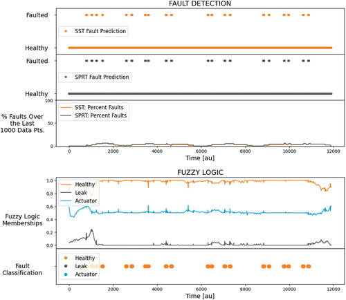
It is imperative to first look at the results from the healthy data in order to validate the fault detection and fuzzy classification methods. Due to the nonlinearities inherent to power changes, the healthy LF data will have more false negative calls than SS operation. Results from the healthy LF operation are shown in Fig. 8. In the top half of the figure, a summary of the fault detection results are shown. The SST and SPRT fault predictions share the plot, which has healthy: SPRT, faulted: SPRT, healthy: SST, and faulted: SST on the y-axis. SST and SPRT are represented by orange and gray, respectively, where a data point is added to indicate whether the algorithm determined the data to be faulted or healthy. Also included in the fault detection results is the percentage of faults over the last 1000 data points (about 27.8 h).

In the healthy LF scenario, the fault detection did a good job of validating the methods. However, it is evident where the power changes occurred based on these results, as false positives occurred at these locations. From the portion of the plot that shows the percentage of faults over the past 1000 data points, one can see that SPRT is more sensitive to these power changes, finding more false positives than SST. SPRT has a maximum value of 30% fault predictions over the previous 1000 data points, where SST has a maximum value of 8%.

Below the fault detection results is the fuzzy logic classification system. The two sections of the fuzzy logic results are the (top) fuzzy logic memberships and (bottom) the fault classification. There are membership values for healthy, leaking TCV, and TCV actuator loss of pressure as represented by orange, gray, and blue, respectively. Memberships are plotted through the entire simulation. The lower portion of the fuzzy logic plot classifies the state of the system only when SST or SPRT determined there was a fault. At the time of a fault prediction, the maximum membership was captured and used as the prediction for the current system state. For each fault called during this simulation, the fuzzy logic successfully classified the system to be healthy, essentially identifying a false positive.

Numerical results from the fault detection are shown in Table II for both SS and LF operations. There was a perfect validation for SS operation, receiving no faults for SST or SPRT. SST outperformed SPRT by receiving less false positive fault predictions. Although the fault detection methodology was not perfect, fuzzy logic acted to verify the presence of a fault and determined the system to be healthy 100% of the time.

TABLE II Summary of Fault Detection Results from Healthy Data

	SST		SPRT
	Total Number of Fault Predictions	Percentage of Faults During Simulation	Total Number of Fault Predictions	Percentage of Faults During Simulation
SS	0	0%	0	0%
LF	356	2.99%	370	3.11%

VI.B. Results from Leaking TCV

Our leaking TCV had a lost flow rate ramped up from 0 to approximately 0.035 g/s, as seen in Fig. 4b. As the degradation increased, the system changed further from its nominal operational parameters. This leak was very small, and was comparable to noise in the flowmeters, especially toward the beginning of the simulation.

The fault detection and fuzzy logic results can be seen for the leaking fault mode during SS operation in Fig. 9, with the same format as Fig. 8. SST and SPRT both have a smooth transition from healthy to faulted. SPRT has one false positive very early in the simulation, and an earlier identification of the fault when compared to SST. This can also be seen in the plot showing the percentage of faults over the last 1000 data points. Fuzzy logic correctly identified the early false positive as healthy and all subsequent fault predictions as leaking. Interestingly, the maximum fuzzy membership became leaking prior to the first SST or SPRT fault prediction.

Fig. 9. Fault detection and fuzzy classification results using leaking SS data.

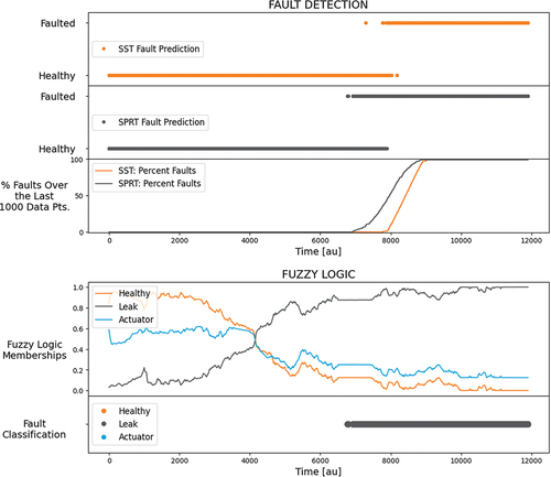
Table III summarizes the results from both SS and LF operations during a TCV leaking degradation. As expected, the total number of faults was greater in LF when compared to SS. However each method was capable of reaching 100% fault predictions over the last 1000 data points.

TABLE III Summary of Fault Detection Results from Leaking Data

	SST		SPRT
	Total Number of Fault Predictions	Percentage of Faults During Simulation	Total Number of Fault Predictions	Percentage of Faults During Simulation
SS	3981	33.46%	4460	37.49%
LF	4557	38.30%	4958	41.67%

VI.C. Results from TCV Actuator Degradation

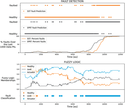
Figure 10 shows the fault detection and fuzzy classification results from an actuator failure in LF operation. The same false positive fault predictions from the healthy LF data were evident in the early stage of the actuator LF data. There was, however, a relatively clean transition toward 100% fault predictions in the second half of the simulation. This was supported by the fuzzy logic classification, where the initial fault predictions were classified as healthy before switching over to actuator once the degradation had progressed sufficiently. Comparing the numbers from Tables III and IV, there generally were more fault predictions from the actuator degradation when compared to the leaking fault.

TABLE IV Summary of Fault Detection Results from Actuator Data

	SST		SPRT
	Total Number of Fault Predictions	Percentage of Faults During Simulation	Total Number of Fault Predictions	Percentage of Faults During Simulation
SS	3277	27.54%	3877	32.59%
LF	3199	26.89%	3835	32.23%

Fig. 10. Fault detection and fuzzy classification results using actuator LF data.

VII. CONCLUSIONS

An iPWR and its associated power plant were modeled based on the NPM in Modelica using the TRANSFORM and Hybrid libraries. The model proved capable of simulating data for SS and operational transients (LF). The effects of two fault modes were simulated in the TCV system. The first degradation mode implemented was a small leak in a TCV. During SS, this leak increased at a linear rate. However, this degradation was more physically motivated during LF operation.

The other degradation acted on the actuator of the valve. In the case where the actuator lost hydraulic pressure, it had less ability to remain open. This was modeled in the second fault mode by adding a multiplication factor between the PID, which controls the TCV actuator position, and the TCV position input. This fault mode became less physically motivated when one noticed that the TCV could still open and close at the same speed during LF. However, the degradation implementation into the iPWR model was overall successful and produced useful data for the purpose of fault and anomaly detection, as well as state classification using fuzzy logic.

Using a NN autoencoder trained with healthy data, two different anomaly detection methods were applied to perform fault monitoring, SST and SPRT. Both anomaly detection routines showed promise for monitoring the imposed TCV degradation modes. Fuzzy logic was used to validate the presence of a fault and to differentiate the two fault modes. The cumulative sum of the autoencoder’s residuals were kept over the last 1000 data points for each variable type besides SG pressure; these cumulative residuals were placed into high, normal, and low membership functions.

Prior knowledge and logic of how these variables would change were used to create rules for calculating system state memberships (healthy, leaking TCV, and TCV actuator loss of pressure). This strategy necessitates a fair amount of prior knowledge, but can create a very powerful and useful tool to identify the current state of the system. In practice, at a commercial NPP, the fault detection and fuzzy logic classification could be used to understand the state of physical aspects and to help determine when maintenance is necessary.

Ongoing work will focus on several areas for further development and improvement: (1) optimizing the SST and SPRT parameters to improve false alarms, particularly during LF transients, (2) developing a single monitoring system to detect TCV degradation or FWP degradation (see Ref. [7] for details on FWP degradation simulation and monitoring), including potentially simultaneous faults in multiple components at once, and (3) estimating the system’s remaining useful life under the degradation of multiple components.

Acknowledgments

We would like to acknowledge and thank Wesley C. Williams of the Advanced Reactor Systems Group at ORNL for his continued assistance with the TRANSFORM package and general support throughout the duration of this project.

This paper was prepared as an account of work sponsored by an agency of the U.S. government. Neither the U.S. government nor any agency thereof, nor any of their employees, makes any warranty, express or implied, or assumes any legal liability or responsibility for the accuracy, completeness, or usefulness of any information, apparatus, product, or process disclosed, or represents that its use would not infringe privately owned rights. Reference herein to any specific commercial product, process, or service by trade name, trademark, manufacturer, or otherwise, does not necessarily constitute or imply its endorsement, recommendation, or favoring by the U.S. government or any agency thereof. The views and opinions of the authors expressed herein do not necessarily state or reflect those of the U.S. government or any agency thereof.

Disclosure Statement

No potential conflict of interest was reported by the author(s).

Additional information

Funding

This work was supported by funding received from the U.S. Department of Energy, Office of Nuclear Energy’s Nuclear Energy University Program under contract no. DE-NE0008975.

References

- Z. FEROZ et al., “Flexible Nuclear Energy for Clean Energy Systems,” presented at Nuclear Innovation: Clean Energy Future (NICE) Future Initiative (2020).
- A. PRAJAPATI, J. BECHTEL, and S. GANESAN, “Condition Based Maintenance: A Survey,” J. Qual. Maint. Eng., 18, 4, 384 (2012); http://doi.org/10.1108/13552511211281552.
- H. KIM, G. NA, and G. HEO, “Application of Monitoring, Diagnosis, and Prognosis in Thermal Performance Analysis for Nuclear Power Plants,” Nucl. Eng. Technol., 46, 6, 737 (2014); http://doi.org/10.5516/NET.04.2014.720.
- “Application Documents for the NuScale US600 Design,” U.S. Nuclear Regulatory Commission (2020); https://www.nrc.gov/reactors/new-reactors/smr/licensing-activities/nuscale/documents.html#dcApp.
- K. FRICK and S. BRAGG-SITTON, “Development of the NuScale Power Module in the INL Modelica Ecosystem,” Nucl. Technol., 207,4, 521 (2020); https://doi.org/10.1080/00295450.2020.1781497.
- M. S. GREENWOOD, “TRANSFORM—TRANsient Simulation Framework of Reconfigurable Models,” ORNL-Modelica/TRANSFORM-Library, github (2017); https://github.com/ORNL-Modelica/TRANSFORM-Library.
- M. SCOTT, “Component Monitoring Strategies for iPWR Plant Systems During Operational Transients,” MS Thesis, University of Tennessee, Nuclear Engineering (2022); https://trace.tennessee.edu/utk_gradthes/7033/.
- D. INGERSOLL et al., “Can Nuclear Power and Renewables Be Friends?,” Proc. ICAPP, Vol. 9 (2015).
- D. BLAHNIK et al., “Insights Gained from Aging Research,” NUREG/CR-5643, U.S. Nuclear Regulatory Commission (1992).
- S. HESLER, “Turbine Steam Valve Diagnostic Testing,” Electric Power Research Institute (2004).
- S. PARKER, “U.S. Steam Turbine Valve Metallurgy Guide,” Electric Power Research Institute (2009).
- K. SOTOODEH, “Actuator Selection and Sizing for Valves,” SN Appl. Sci., 1, 1207 (2019); http://doi.org/10.1007/s42452-019-1248-z.
- M. SCOTT and J. COBLE, “Toward Health Management of Active Components During Operational Transients in SMRs,” presented at the Annual Mtg. of the American Nuclear Society (2022).
- K. CHOI et al., “Deep Learning for Anomaly Detection in Time-Series Data: Review, Analysis, and Guidelines,” IEEE Access, 9, 120043 (2021); http://doi.org/10.1109/ACCESS.2021.3107975.
- D. HU et al., “Anomaly Detection of Power Plant Equipment Using Long Short-Term Memory Based Autoencoder Neural Network,” Sensors, 20, 21, 120043 (2020); http://doi.org/10.3390/s20216164.
- T. WEN and R. KEYES, “Time Series Anomaly Detection Using Convolutional Neural Net-Works and Transfer Learning,” presented at the AI for Internet of Things Workshop (IJCAI 2019) (2019); https://arxiv.org/pdf/1905.13628.
- M. BRAEI and S. WAGNER, “Anomaly Detection in Univariate Time-Series: A Survey on the State-of-the-Art,” CoRR, abs/2004.00433 (2020); https://arxiv.org/abs/2004.00433.
- A. WALD, “Sequential Tests of Statistical Hypotheses,” Ann. Math. Statist., 16, 2, 117 (1945); http://doi.org/10.1214/aoms/1177731118.
- L. H. TSOUKALAS and R. E. UHRIG, Fuzzy and Neural Approaches in Engineering, Wiley Interscience (1997).