MULTI-PRED: A Software Module for Predictive Modeling of Coupled Multi-Physics Systems

Abstract

The software module MULTI-PRED implements the methodology for predictive modeling of coupled multi-physics systems (PM-CMPS) formulated by Cacuci [Ann. Nucl. Energy, Vol. 70, p, 266 (2014)]. This methodology fully takes into account the coupling terms between the systems but requires only the computational resources that would be needed to perform predictive modeling on each system separately. The PM-CMPS methodology uses the maximum entropy principle to construct an optimal approximation of the unknown a priori distribution based on a priori known mean values and uncertainties characterizing the experimental and computational parameters and results of interest responses called for the multi-physics models under consideration. This maximum entropy a priori distribution is combined, using Bayes’ theorem, with the likelihood provided by the multi-physics simulation models to obtain a formal posterior distribution. Subsequently, the posterior distribution thus obtained is evaluated using the saddle-point method to obtain analytical expressions for the optimally predicted values for the multi-physics model parameters and responses along with corresponding reduced uncertainties. Noteworthy, the predictive modeling methodology for the coupled systems is constructed such that the systems can be considered sequentially rather than simultaneously, while preserving exactly the same results as if the systems were treated simultaneously. Consequently, very large coupled systems, which could perhaps exceed available computational resources if treated simultaneously, can be treated with the PM-CMPS methodology presented in this work sequentially and without any loss of generality or information, requiring just the resources that would be needed if the systems were treated sequentially.

The PM-CMPS methodology can be applied to reduce uncertainties in both forward and inverse problems. Three demonstration problems are provided to illustrate the application of the PM-CMPS methodology. The first problem presents the application of the PM-CMPS methodology to a simple particle diffusion problem which admits a closed-form analytical solution which facilitates a rapid understanding of this methodology and its predicted results. The second demonstration problem presents the application of the PM-CMPS methodology to the problem of inverse prediction, from detector responses in the presence of counting uncertainties, of the thickness of a homogeneous slab of material containing uniformly distributed gamma-emitting sources for optically thin and thick slabs. This problem highlights the essential role played by the relative uncertainties (or, conversely, accuracies) of measured and computed responses. The third demonstration problem presents the application of the PM-CMPS methodology to the F-Area cooling towers at the Savannah River National Lab. This problem demonstrates that the PM-CMPS methodology reduces the predicted response uncertainties not only at locations where measurements are available, but also at locations where measurements are not available.

MULTI-PRED is written in Fortran and runs on Linux and Windows systems. A C++ version will also become available.

Keywords:

• Predictive modeling
• data assimilation
• model calibration
• reduced predicted uncertainties
• optimally predicted best-estimate values for mode parameters and responses

I. INTRODUCTION

The results of measurements inevitably reflect the influence of experimental errors, imperfect instruments, and imperfectly known calibration standards. Around any reported experimental value, therefore, there always exists a range of values that may also be plausibly representative of the true but unknown value of the measured quantity. On the other hand, computations are also imperfect, since they are afflicted by errors stemming from numerical procedures, uncertain model parameters, boundary and initial conditions, and/or imperfectly known physical processes or problem geometry. Therefore, nominal values for experimentally measured or computed quantities are insufficient, by themselves, for applications. The quantitative uncertainties accompanying the measurements and computations are also needed, along with the respective nominal values. Extracting best-estimate values for model parameters and predicted results (responses), together with best-estimate uncertainties for these parameters and responses, requires the combination of experimental and computational data and their uncertainties. This combination process often requires reasoning from incomplete, error-afflicted, and occasionally, discrepant information.

The discrepancies between experimental and computational results provide the basic motivation for performing quantitative model verification, validation, qualification, and predictive estimation. Loosely speaking, code verification means: “Are you solving the mathematical model correctly?” Code validation means: “Does the model represent reality?” Code qualification means certifying that a proposed simulation/design methodology/system satisfies all performance and safety specifications. Model validation addresses issues of (1) assessing model accuracy when several system response quantities have been measured and compared and (2) comparing system response quantities from multiple realizations of the experiment with computational results that are characterized by probability distributions. Model validation and qualification require selected benchmarking, including sensitivity and uncertainty analyses.

Predictive modeling commences with the identification and characterization of uncertainties from all steps in the sequence of modeling and simulation processes that lead to a computational model prediction. This includes (1) data error or uncertainty (input data such as cross sections; model parameters such as reaction-rate coefficients, initial conditions, and boundary conditions; and forcing functions such as external loading), (2) numerical discretization error, and (3) uncertainty in (e.g., lack of knowledge of) the processes being modeled. The result of the predictive modeling analysis is a probabilistic description of possible future outcomes based on all recognized errors and uncertainties.

Predictive modeling combines/assimilates computational and experimental information using response sensitivities to perform model calibration, model extrapolation, and estimation of the validation domain. Model calibration addresses the integration of experimental data for the purpose of updating the data of the computer model. Important components include the estimation of discrepancies in the data and of the biases between model predictions and experimental data. The state-of-the-art of model calibration is fairly well developed, but current methods are still hampered in practice by the significant computational effort required. Reducing the computational effort is paramount, and methods based on adjoint models show great promise in this regard. Model extrapolation addresses the prediction uncertainty in new environments or conditions of interest, including both untested parts of the parameter space and higher levels of system complexity in the validation hierarchy. Extrapolation of models and the resulting increase of uncertainty are poorly understood, particularly the estimation of uncertainty that results from nonlinear coupling of two or more physical phenomena that were not coupled in the existing validation database. The quantification of the validation domain underlying the models of interest requires estimation of contours of constant uncertainty in the high-dimensional space that characterizes the application of interest. In practice, this involves the identification of areas where the predictive estimation of uncertainty meets specified requirements for the performance, reliability, or safety of the system of interest.

The software module MULTI-PRED implements the methodology for predictive modeling of coupled multi-physics systems (PM-CMPS) formulated by Cacuci.¹ The PM-CMPS methodology generalizes the work of Cacuci and Ionescu-Bujor^2,3 on predictive modeling of a single time-dependent multi-physics system, and also generalizes and significantly extends the data adjustment methods customarily used in nuclear engineering, as well as those underlying the so-called 4D-VAR data assimilation procedures in the geophysical sciences.^4,5 The PM-CMPS provides a quantitative indicator, constructed from sensitivity and covariance matrices, for determining the consistency (agreement or disagreement) among the a priori computational and experimental data (parameters and responses). This consistency indicator measures, in the corresponding metric, the deviations between the experimental and nominally computed responses. Note that this consistency indicator can be evaluated directly from the originally given data (i.e., given parameters and responses, together with their original uncertainties) once the response sensitivities have been computed. Preferably, the PM-CMPS utilizes the exactly and efficiently computed response sensitivities using the adjoint sensitivity analysis methodology as generally formulated by Cacuci.^6–11 When the numerical value of this consistency indicator is close to unity (per degrees of freedom), the respective data are considered to be consistent within the respective error norms (usually under quadratic loss). However, when the numerical value of this consistency indicator differs considerably from unity, which usually occurs when the distance between the mean values of two (sets of) measurements or two (sets of) computations of the same quantity are larger than the sum of the two accompanying standard deviations, the respective (measured of computed) data points are considered to be inconsistent or discrepant. This means that there is a nonzero probability that two nondiscrepant (i.e., belonging to the same distribution) measurements that are separated by more than 2σ (thus giving the appearance of being discrepant) could actually occur in practice. Recall that for a Gaussian sampling distribution, the probability that two equally precise measurements would be separated by more than 2σ is 15.7%. However, this probability is rather small; therefore, it is much more likely that apparently discrepant data actually indicate the presence of unrecognized errors. Methods for treating unrecognized errors have been developed by Cacuci and Ionescu-Bujor,¹² by applying the maximum entropy principle under quadratic loss to the discrepant data.

The PM-CMPS methodology is constructed such that the systems can be treated sequentially rather than simultaneously, while preserving exactly the same results as if the systems had been treated simultaneously. Consequently, very large coupled systems, which could perhaps exceed available computational resources if treated simultaneously, can be treated with the PM-CMPS methodology sequentially, without any loss of generality or information, requiring just the resources that would be needed as if the systems had been treated separately. The PM-CMPS methodology has been successfully applied to reducing the predicted uncertainties in model parameters and responses in several forward and inverse problems.^13–18 The MULTI-PRED software module provides three illustrative problems: (1) a simple neutron diffusion problem,¹⁹ (2) an inverse problem in particle transport,¹⁸ and (3) a predictive modeling of the F-Area cooling towers at the Savannah River National Laboratory.^16,17 Sections II and III describe the quantities required as inputs to MULTI-PRED, along with the optimally predicted best-estimate values for the model responses and model parameters, with reduced predicted uncertainties, which are obtained as the outputs of MULTI-PRED.

II. PM-CMPS: MATHEMATICAL FRAMEWORK

II.A. MULTI-PRED Input: A Priori Information for Two Multi-Physics Models

Consider a multi-physics model, henceforth called model A comprising system (model) parameters . Model A is used to compute results, henceforth called responses, which can also be measured experimentally. Consider now a second physical system, henceforth called model B, comprising system (model) parameters , and which is also used to compute responses that can be measured experimentally. Model A and model B are considered to be coupled. In reactor analysis and design, for example, model A may comprise the neutron transport and depletion equations which are coupled to model B which computes the thermal-hydraulic conservation (mass, momentum, energy) equations.

Consider next that there are experimentally measured responses associated mostly, but not necessarily exclusively, with model A. Furthermore, consider also that there are experimentally measured responses associated mostly, but not necessarily exclusively, with model B. For example, measurement of reaction rates and power (or flux) distributions could be considered to be responses of type , while measurements of flow rates and temperature distributions could be considered responses of type . In the same spirit, cross sections can be considered to be model parameters of type , while heat transfer correlations can be considered model parameters of type . Parameters modeling the geometry of the system (e.g., rod and assembly dimensions, core dimensions), for example, could be considered to belong to either type of model parameters (i.e., either or ), since they affect both the neutron transport equation and the thermal-hydraulic conservation equations.

In practice, the values of the parameters and are determined experimentally. Therefore, these parameters cannot be known exactly, but can be considered to behave stochastically, obeying some probability distribution function which is seldom known. Such stochastic quantities will be called variates in this work; thus, the parameters and as well as the measured responses and are variates. To simplify the mathematical derivations to follow in this section, the model parameters will be considered to constitute the components of the (column) vector , defined as

(1)

while the model parameters will be considered to constitute the components of the (column) vector defined as

(2)

By convention, all of the vectors considered in this work (e.g., and ) are column vectors. A dagger will be used to denote transposition; thus, the quantities and are row vectors. Similarly, the experimentally measured responses will be considered to be components of the column vector:

(3)

while the experimentally measured responses will be considered to be components of the column vector:

(4)

Most generally, the parameters and , as well as the responses and can be considered to obey some a priori probability distribution function . For large-scale systems, as customarily encountered in practice, the probability distribution is unknown. The information usually available in practice comprises the mean values of the model parameters and responses together with the corresponding uncertainties (standard deviations and, occasionally, correlations) about the respective mean values. For notational simplicity, angular brackets will be used to denote the integral of the quantity over the joint probability distribution , i.e.,

(5)

Using the above convention, the mean values of the model parameters will be denoted using the superscript zero, i.e., as ; these mean values are considered to constitute the components of the vector defined as

(6)

Similarly, the mean values of the parameters are considered to be known and will be denoted as . These mean values are considered to be the components of the vector defined as

(7)

The parameters’ second-order central moments, namely the standard deviations and correlations, are also considered to be known. For the parameters , the second-order central moments are the components of covariance matrices defined as

(8)

while the second-order central moments (i.e., the standard deviations and correlations) for the parameters form covariance matrices defined as

(9)

In general, the components of the vectors and may be correlated. The correlations among the parameters and are quantified by correlation matrices defined as

(10)

The experimentally measured responses are also considered to be characterized by known mean measured values and measured variances and covariances. Thus, for the experimentally measured responses , the mean measured values will be denoted as and will be considered to constitute the components of the vector defined as

(11)

while the corresponding measured covariance matrix, denoted as , is defined as

(12)

Similarly, the experimentally measured responses are characterized by mean measured values, denoted as , and constituting the components of the vector defined as

(13)

and by the measured covariance matrix defined as

(14)

Furthermore, the responses and may also be correlated; such correlations would be quantified by correlation matrices defined as

(15)

In the most general case, correlations may also exist among all parameters and responses. Such correlations would be quantified through matrices defined as follows:

(16)

(17)

(18)

and

(19)

II.B. MULTI-PRED Output: Optimally Predicted Values of Model Parameters and Responses

The following quantities are computed and provided as outputs of MULTI-PRED:

1. Covariance matrices of the computed responses for model A arising from the uncertainties in the model parameters of model A:

2. Covariance matrices of the computed responses for model B arising from the uncertainties in the model parameters of model B:

3. Correlation matrices of the computed responses for models A and B arising from the uncertainties in the model parameters of models A and B:

   (22)

4. Optimally predicted best-estimate values for the parameters of model A (model calibration):

   (23)

5. Optimally predicted best-estimate values for the parameters of model B (model calibration):

   (24)

6. Optimally predicted best-estimate values for the responses of model A:

7. Optimally predicted best-estimate values for the responses of model B:

8. Optimally predicted best-estimate values for components of the covariance matrix for the parameters of model A:

9. Optimally predicted best-estimate values for the components of the predicted covariance matrix for the responses of model A:

   (28)

10. Optimally predicted best-estimate values for the components of the predicted correlation matrix for the parameters and responses of model A:

11. Optimally predicted best-estimate values for the components of the predicted covariance matrix for the parameters of model B:

12. Optimally predicted best-estimate values for the components of the predicted covariance matrix for the responses of model B are obtained as

13. Optimally predicted best-estimate values for the components of the predicted correlation matrix for the parameters and the responses of model B:

14. Optimally predicted best-estimate values for the components of the predicted correlation matrix for the parameters of model A and the parameters of model B:

15. Optimally predicted best-estimate values for the components of the predicted correlation matrix for the parameters of model A and the responses of model B:

    (34)

16. Optimally predicted best-estimate values for the components of the predicted correlation matrix for the parameters of model B and the responses of model A:

17. Optimally predicted best-estimate values for the components of the predicted correlation matrix for the responses of model A and the responses of model B:

18. The validation metric :

    (37)

The validation metric can be evaluated directly from the originally given data (i.e., from given parameters and responses, together with their original uncertainties). The validation metric is distributed according to the (chi-square)-distribution with degrees of freedom of the continuous variable and is defined as

The mean and variance of are and . Since the -distribution is a measure of the deviation of a true distribution (in this case, the distribution of experimental responses) from the hypothetic one (in this case, a Gaussian), the value of computed using Eq. (37) provides a very valuable quantitative indicator for investigating the agreement between the computed and experimental responses, measuring essentially the consistency of the experimental responses with the model parameters.

The various quantities appearing in Eqs. (20) through (37) are defined as follows:

1. The matrices , , , and comprise first-order response-derivatives with respect to the model parameters, computed at the nominal parameter values , and are defined as follows:

(39)

2. The vectors and measure the differences (deviations) between the computed and measured responses, and are defined as follows:

(41)

3. The matrix , having , is actually the covariance matrix of the vector of response deviations for model A, i.e.,

(42)

4.  The matrix , having , is actually the covariance matrix of the vector of response deviations for model B, i.e.,

(43)

5.  The matrix , having dim , is actually the correlation matrix between the vector of response deviations for model A and model B, i.e.,

(44)

and

(45)

6. The matrices , , and are defined as follows:

(46)

(47)

(48)

and

(49)

7. The vectors , , , , , , , and are defined as follows:

(50)

(51)

(52)

(53)

(54)

(55)

(56)

and

(57)

II.C. Discussion and Particular Cases

The derivations in Sec. II.B were carried out in the response space because in large-scale practical problems, the number of measured responses is smaller than the number of model parameters. The only matrix inversions required are the inversion of the matrix of size in Eq. (46) and the inversion of the matrix , which is of size in Eq. (49). Both of these matrix inversions are performed in the respective response spaces.

The PM-CMPS methodology can also be used if one starts with the data assimilation and model calibration for one of the models (either model A or model B) and subsequently couples the second model to the first one. Without the PM-CMPS methodology, when the second model (e.g., model B) is coupled to the first one (e.g., model A), both models would have to be calibrated anew, simultaneously, and the work performed initially for calibrating model A alone would become useless. Using the PM-CMPS methodology, however, the work initially performed for calibrating model A would not become useless, but would simply be augmented by the specific additional terms arising from model B, thus performing PM-CMPS in a sequential and more efficient way.

It is also important to note that the explicit separation, in Eq. (37), of contributions from model A and model B to the overall validation metric enables the explicit evaluation of adding or subtracting measured responses. Large contributions to indicate that the respective responses may be inconsistent or discrepant, and such discrepancies warrant further investigations.

It often happens in practice that, after one has already performed a model calibration, e.g., using model A (involving model parameters and experimentally measured responses ), additional measurements may become available and/or additional parameters (which were not considered in the initial data assimilation/model calibration/predictive modeling procedure) may need to be taken into account (e.g., model parameters for which quantified uncertainties became available only after the initial data assimilation/model calibration/predictive modeling procedure was already performed), all for the same model A. The PM-CMPS predictive modeling methodology can also be used as a most efficient procedure for systematically adding or subtracting responses and/or parameters for performing a subsequent data assimilation/model calibration/predictive modeling procedure on the same model, without “wasting” the information already obtained in previous predictive modeling computations that involved a different (higher or lower) number of responses and/or model parameters. Adding and/or subtracting measurements (responses) and/or model parameters to the same model without needing to discard previous predictive modeling computations are described in Secs. III.C.1, III.C.2, and III.C.3 as particular cases of the general PM-CMPS methodology.

II.C.1. Predictive Modeling for a Single Multi-Physics Model

In the case of applying the PM-CMPS methodology for the predictive modeling of a single multi-physics model (e.g., model A, involving model parameters and experimentally measured responses ), the predictive modeling equations Eqs. (20) through (37) reduce to the final results presented originally by Cacuci and Ionescu-Bujor,³ namely,

(58)

(59)

(60)

(61)

and

(62)

Note that if the model is perfect (i.e., and ), then Eqs. (58) through (62) would yield and , predicted perfectly without any accompanying uncertainties (i.e., , , and ). In other words, for a perfect model, the PM-CMPS methodology predicts values for the responses and the parameters that coincide with the model’s values (assumed to be perfect), and the experimental measurements would have no effect on the predictions (as would be expected, since imperfect measurements could not possibly improve the perfect model’s predictions).

On the other hand, if the measurements are perfect (i.e., and ), but the model is imperfect, then Eqs. (58) through (62) would yield , , , and . In other words, in the case of perfect measurements, the PM-CMPS predicted values for the responses would coincide with the measured values (assumed to be perfect), but the model’s uncertain parameters would be calibrated by taking the measurements into account to yield improved nominal values and reduced parameter uncertainties.

II.C.2. Predictive Modeling for Model A with Additional Parameters, But No Additional Responses

In this case, the predictive modeling formulation in the response space allows the consideration of additional parameters for a model without increasing the size of the matrix to be inverted. This is clearly demonstrated as Eqs. (20) through (57) become

(63)

(64)

(65)

(66)

(67)

(68)

(69)

(70)

(71)

(72)

(73)

(74)

(75)

(76)

(77)

and

(78)

II.C.3. Predictive Modeling for Model A with Q Additional Responses, But No Additional Parameters

In this case, Eqs. (20) through (57) become

(79)

(80)

(81)

(82)

(83)

(84)

(85)

(86)

(87)

(88)

(89)

(90)

(91)

(92)

(93)

(94)

(95)

(96)

(97)

(98)

and

(99)

Note also that (to first order in response sensitivities) the covariance matrices of the computed responses arising from the uncertainties in the model parameters become

(100)

(101)

and

(102)

III. MULTI-PRED CODE MODULE

The equations expressing the results of the PM-CMPS methodology developed by Cacuci¹ namely, Eqs. (20) through (57), have been programed in the computational software module MULTI-PRED. All routines in MULTI-PRED are written in Fortran 90 and are compatible with most Linux systems, performing predictive modeling computations for the following four cases:

• Case 1: One Multi-Physics Model—predictive modeling solely for model A with model parameters and measured responses

• Case 2: One Multi-Physics Model with Additional Model Parameters—predictive modeling for model A with additional model parameters, but no additional responses

• Case 3: One Multi-Physics Model with Additional Model Responses—predictive modeling for model A with additional responses, but no additional parameters

• Case 4: Two Coupled Multi-Physics Models—predictive modeling for model A coupled with model B.

III.A. Fortran Source Code for the Program MULTI-PRED

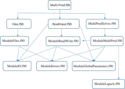
The program MULTI-PRED includes the following routines and modules:

1. main program: multi-pred.f90

2. module: ModuleGlobalParameters.f90

3. module: ModuleIO.f90

4. module: ModuleErrors.f90

5. subroutine: Files.f90

6. module: ModuleFiles.f90

7. subroutine: ReadInput.f90

8. module: ModuleReadWrite.f90

9. subroutine: MultiPredSolver.f90

10. module: ModuleMultiPred.f90

11. module: ModuleLapack.f90

The structure of the MULTI-PRED software module is organized as shown in Fig. 1.

Fig. 1. MULTI-PRED code structure.

III.B. Directories

The computational software module MULTI-PRED comprises the following directories:

1. multi-pred/source/: This folder contains the source codes.

2. multi-pred/examples/: This folder contains five examples specified in the following subfolders:

   1. ../Neutron_Diffusion_Model_Case_1/: This folder contains the input/output (I/O) files for MULTI-PRED case 1 for a neutron diffusion model.

   2. ../Cooling_Tower_Model_Case_1/: This folder contains the I/O files for MULTI-PRED case 1 for the SRNL cooling tower model.

   3. ../Cooling_Tower_Model_Case_2/: This folder contains the I/O files for MULTI-PRED case 2 for the SRNL cooling tower model.

   4. ../Cooling_Tower_Model_Case_3/: This folder contains the I/O files for MULTI-PRED case 3 for the SRNL cooling tower model.

   5. ../Cooling_Tower_Model_Case_4/: This folder contains the I/O files for MULTI-PRED case 4 for the SRNL cooling tower model.

3. multi-pred/matrix_positive_definite_test/: This folder contains the source code for a standalone program used to test if a symmetric matrix is positive definite (SPD).

Note that the covariance matrices , , , and must be SPD matrices. This program computes the Cholesky factorization of the matrix being tested. If it can be factorized, the program returns a flag indicating that the tested matrix is SPD. Running this test standalone program is optional, since the Cholesky factorization has also been implemented in MULTI-PRED. Also included in this folder is a large-scale matrix used for the SPD test. This matrix is a large SPD matrix, with a seemingly random sparsity pattern. It has a dimension of 60 000 × 60 000 with 410 077 nonzero elements.^a

III.C. Code Compilation and Execution

Compilation and execution are accomplished as follows:

1. Compile the software program in Linux. Enter the multi-pred/source/ directory and use the command make. An executable named multi-pred will be generated under the source directory. The compiler used in the makefile is ifort (version 12.1.6 and above). It can also be compiled with gfortran (version 4.47 and above). An example makefile with the gfortran compiler, named makefile.gfortran, is also included in the source directory.

2. Run the program. To run the program, copy the executable multi-pred into the example directories, then use the command: /multi-pred superfile.inp where the argument superfile.inp contains all the I/O file names. Output files will be generated in the respective example folders.

III.D. Input and Output File Organization

This section describes the I/O files within the MULTI-PRED module.

III.D.1. Super-File

The MULTI-PRED super-file is a text file that contains the names of I/O files and organizes the individual files for I/O operations. This super-file is read from the command line (UNIT = 5) as an argument. The first line of the super-file is reserved for an identifier card, MultiPredSup. After the identifier line, each subsequent line is preceded by a category code and a file name. The category code and file name have to be enclosed in single quotes. The file names can be changed by the user. The second line of the super-file is also reserved for the dims category; the corresponding input file defines the dimensions of the matrices and vectors used in MULTI-PRED. The lines after the second line are for data files. There are no restrictions regarding the order of the data files and their corresponding categories. Table I shows the format and complete list of super-files for MULTI-PRED case 4: Two Coupled Multi-Physics Models.

TABLE I MultiPredSup Super-File Format for MULTI-PRED Case 4: Two Coupled Multi-Physics Models

Category	File Name
‘dims’	‘dimensions.inp’
‘a_nom’	‘a.inp’
‘r_mea’	‘rm.inp’
‘r_com’	‘rc.inp’
‘C_aa’	‘Caa.inp’
‘C_ar’	‘Car.inp’
‘C_rr’	‘Crr.inp’
‘S_ra’	‘Sra.inp’
‘b_nom’	‘b.inp’
‘q_mea’	‘qm.inp’
‘q_com’	‘qc.inp’
‘C_bb’	‘Cbb.inp’
‘C_bq’	‘Cbq.inp’
‘C_qq’	‘Cqq.inp’
‘S_qb’	‘Sqb.inp’
‘C_ab’	‘Cab.inp’
‘C_aq’	‘Caq.inp’
‘C_br’	‘Cbr.inp’
‘C_rq’	‘Crq.inp’
‘S_rb’	‘Srb.inp’
‘S_qa’	‘Sqa.inp’
‘a_BE’	‘aBE.out’
‘r_BE’	‘rBE.out’
‘C_aaBE’	‘CaaBE.out’
‘C_rrBE’	‘CrrBE.out’
‘C_arBE’	‘CarBE.out’
‘Crr_comp’	‘Crrcomp.out’
‘b_BE’	‘bBE.out’
‘q_BE’	‘qBE.out’
‘C_bbBE’	‘CbbBE.out’
‘C_qqBE’	‘CqqBE.out’
‘C_bqBE’	‘CbqBE.out’
‘Cqq_comp’	‘Cqqcomp.out’
‘C_abBE’	‘CabBE.out’
‘C_aqBE’	‘CaqBE.out’
‘C_brBE’	‘CbrBE.out’
‘C_rqBE’	‘CrqBE.out’
‘Crq_comp’	‘Crqcomp.out’
‘chi2’	‘chi2.out’

III.D.2. Contents and Organization of I/O Files

The file dimensions.inp defines the following important control variables.

CaseNumber—Multi-Pred case selection:

: number of parameters for model A

: number of responses for model A

: number of additional parameters for model A (case 2) or the number of parameters of model B (case 4)

: number of additional responses for model A (case 3) or the number of responses of model B (case 4).

All data files are in the sparse triplet matrix file format, which is a commonly used ASCII file format for storing sparse matrices and is compatible with most files in the Matrix Market format.

The sparse triplet data structure simply records, for each nonzero entry of the matrix, the row, column, and value. The general format is as follows:

Line 1: M N Nz

Line 2: Row_index Col_index Val

Line 3: Row_index Col_index Val

… … … …

Line Nz + 1: Row_index Col_index Val

In the above format, the quantities M and N denote, respectively, the number of rows and columns in the original full matrix; Nz denotes total number of nonzero elements in the matrix; Row_index and Col_index denote the row and column indices of each nonzero element; and VAL denotes the value of the nonzero element.

Table II describes the contents of the I/O files specified within the MULTI-PRED super-files for case 4: Two Coupled Multi-Physics Models.

TABLE II Summary of I/O Files for MULTI-PRED Case 4: Two Coupled Multi-Physics Models

File	Unit	I/O	Corresponding Vector/Matrix	Description
superfile.inp	5	Input		File organization
dimensions.inp	20	Input		Defines the case selection and dimensions control
a.inp	21	Input		Nominal values of Na parameters of model A
rm.inp	22	Input		Nominal values of Nr measured responses of model A
rc.inp	23	Input		Nominal values of Nr computed responses of model A
Caa.inp	24	Input		Covariance matrix of Na parameters of model A
Car.inp	25	Input		Correlations between Na parameters and Nr responses of model A
Crr.inp	26	Input		Covariance matrix of Nr responses of model A
Sra.inp	27	Input		Absolute sensitivities of Nr responses of model A with respect to Na parameters of model A
b.inp	31	Input		Nominal values of Na parameters of model B
qm.inp	32	Input		Nominal values of Nq measured responses of model B
qc.inp	33	Input		Nominal values of Nq computed responses of model B
Cbb.inp	34	Input		Covariance matrix of Nb parameters of model B
Cbq.inp	35	Input		Correlations between Nb parameters and Nq responses of model B
Cqq.inp	36	Input		Covariance matrix of Nq responses of model B
Sqb.inp	37	Input		Absolute sensitivities of Nq responses of model B with respect to Nb parameters of model B
Cab.inp	41	Input		Correlation matrix between the Na parameters of model A and the Nb parameters of model B
Caq.inp	42	Input		Correlation matrix between the Na parameters and of model A and Nq responses of model B
Cbr.inp	43	Input		Correlation matrix between the Nb parameters of model B and Nr responses of model A
Crq.inp	44	Input		Correlation matrix of between Nr responses of model A and Nq responses of model B
Srb.inp	45	Input		Absolute sensitivities of Nr responses of model A with respect to Nb parameters of model B
Sqa.inp	46	Input		Absolute sensitivities of Nq responses of model B with respect to Na parameters of model A
aBE.out	51	Output		Best-estimate nominal values of parameters of model A
rBE.out	52	Output		Best-estimate nominal values of responses of model A
CaaBE.out	53	Output		Predicted covariance matrix of Na parameters of model A
CrrBE.out	54	Output		Predicted covariance matrix of Nr responses of model A
CarBE.out	55	Output		Predicted correlation matrix between the Na parameters and Nr responses of model A
Crrcomp.out	56	Output		Covariance matrix of Nr computed responses of model A
bBE.out	61	Output		Best-estimate nominal values of parameters of model B
qBE.out	62	Output		Best-estimate nominal values of responses of model B
CbbBE.out	63	Output		Predicted covariance matrix of Nb parameters of model B
CqqBE.out	64	Output		Predicted covariance matrix of Nq responses of model B
CbqBE.out	65	Output		Predicted correlation matrix between the Nb parameters and Nq responses of model B
Cqqcomp.out	66	Output		Covariance matrix of Nq computed responses of model B
CabBE.out	71	Output		Predicted correlation matrix between the Na parameters of model A and the Nb parameters for model B
CaqBE.out	72	Output		Predicted correlation matrix between the Na parameters and of model A and Nq responses of model B
CbrBE.out	73	Output		Predicted correlation matrix between the Nb parameters of model B and Nr responses of model A
CrqBE.out	74	Output		Predicted correlation matrix of between Nr responses of model A and Nq responses of model B
Crqcomp.out	75	Output		Correlation matrix of Nr computed responses of model A and Nq computed responses of model B
chi2.out	76	Output	, scalar	Value of the consistency indicator

III.D.3. Input Data Files for MULTI-PRED Case 4

Table III presents the 20 input files required for MULTI-PRED case 4.

TABLE III Input Data Files for MULTI-PRED Case 4

Input Data Files for Model A	Input Data Files for the Coupled Matrices Between Model A and Model B	Input Data Files for Model B
a.inp	–	b.inp
rm.inp	–	qm.inp
rc.inp	–	qc.inp
Caa.inp	Cab.inp	Cbb.inp
Car.inp	Caq.inp, Cbr.inp	Cbq.inp
Crr.inp	Crq.inp	Cqq.inp
Sra.inp	Sqa.inp, Srb.inp	Sqb.inp

Notes

^a Refer to the following website http://www.cise.ufl.edu/research/sparse/matrices/Andrews/Andrews for detailed information about this matrix.

References

- D. G. CACUCI, “Predictive Modeling of Coupled Multi-Physics Systems: I. Theory,” Ann. Nucl. Energy, 70, 266, (2014); https://doi.org/10.1016/j.anucene.2013.11.027.
- D. G. CACUCI and M. IONESCU-BUJOR, “Sensitivity and Uncertainty Analysis, Data Assimilation and Predictive Best-Estimate Model Calibration,” Handbook of Nuclear Engineering, Vol. 3, Chap. 17, pp. 1913–2051, D. G. CACUCI, Ed., Springer New York/ Berlin (2010); ISBN: 978-0-387-98150-5.
- D. G. CACUCI and M. IONESCU-BUJOR, “Best-Estimate Model Calibration and Best-Estimate Prediction Through Experimental Data Assimilation—I: Mathematical Framework,” Nucl. Sci. Eng., 165, 1, 18 (2010), https://doi.org/10.13182/NSE09-37B.
- Data Assimilation: Making Sense of Observations, W. LAHOZ, B. KHATTATOV, and R. MÉNARD, Eds., Springer Verlag, Berlin.
- D. G. CACUCI, M. I. NAVON, and M. IONESCU-BUJOR, Computational Methods for Data Evaluation and Assimilation, Chapman & Hall/CRC, Boca Raton, Florida (2013).
- D. G. CACUCI, “Sensitivity Theory for Nonlinear Systems: I. Nonlinear Functional Analysis Approach,” J. Math. Phys., 22, 2794, (1981); https://doi.org/10.1063/1.525186.
- D. G. CACUCI, “Sensitivity Theory for Nonlinear Systems: II. Extensions to Additional Classes of Responses” J. Math. Phys., 22, 2803, (1981); https://doi.org/10.1063/1.524870.
- D. G. CACUCI, “The Forward and the Adjoint Methods of Sensitivity Analysis,” Uncertainty Analysis, Y. RONEN, Ed., Chap. 3, pp. 71–144. CRC Press, Inc, Boca Raton, Florida (1988).
- D. G. CACUCI, Sensitivity and Uncertainty Analysis: Theory, Vol. 1, Chapman & Hall/CRC, Boca Raton, Florida (2003).
- D. G. CACUCI, “Second-Order Adjoint Sensitivity Analysis Methodology (2nd-ASAM) for Computing Exactly and Efficiently First- and Second-Order Sensitivities in Large-Scale Linear Systems: I. Computational Methodology,” J. Comp. Phys., 284, 687, (2015); https://doi.org/10.1016/j.jcp.2014.12.042.
- D. G. CACUCI, “Second-Order Adjoint Sensitivity Analysis Methodology (2nd-ASAM) for Large-Scale Nonlinear Systems—I: Theory,” Nucl. Sci. Eng., 184, 16, (2016); https://doi.org/10.13182/NSE16-16.
- D. G. CACUCI and M. IONESCU-BUJOR, “On the Evaluation of Discrepant Scientific Data with Unrecognized Errors,” Nucl. Sci. Eng., 165, 1, (2010); https://doi.org/10.13182/NSE09-37A.
- M. C. BADEA, D. G. CACUCI, and A. F. BADEA, “Best-Estimate Predictions and Model Calibration for Reactor Thermal-Hydraulics,” Nucl. Sci. Eng., 172, 1, (2012); https://doi.org/10.13182/NSE11-10.
- E. ARSLAN and D. G. CACUCI, “Predictive Modeling of Liquid-Sodium Thermal-Hydraulics Experiments and Computations,” Ann. Nucl. Energy, 63C, 355, 2014 (2014); https://doi.org/10.1016/j.anucene.2013.07.029.
- D. G. CACUCI and E. ARSLAN, “Reducing Uncertainties Via Predictive Modeling: FLICA4 Calibration Using BFBT Benchmarks,” Nucl. Sci. Eng., 176, 339, (2014); https://doi.org/10.13182/NSE13-31.
- D. G. CACUCI and R. FANG, “Predictive Modelling of a Paradigm Mechanical Cooling Tower: I. Adjoint Sensitivity Model,” Energies, 9, 718, (2016); https://doi.org/10.3390/en9090718.
- R. FANG, D. G. CACUCI, and M. C. BADEA, “Predictive Modelling of a Paradigm Mechanical Cooling Tower: II. Optimal Best-Estimate Predictions with Reduced Uncertainties,” Energies, 9, 747, (2016); https://doi.org/10.3390/en9090747.
- D. G. CACUCI, “Inverse Predictive Modeling of Radiation Transport Through Optically Thick Media in the Presence of Counting Uncertainties,” Nucl. Sci. Eng, 186, 199, (2017); https://doi.org/10.1080/00295639.2017.1305244.
- D. G. CACUCI and M. C. BADEA, “Predictive Modelling of Coupled Multi-Physics Systems: II. Illustrative Application to Reactor Physics,” Ann. Nucl. Energy, 70, 279, (2014); https://doi.org/10.1016/j.anucene.2013.11.025.