
 ?Mathematical formulae have been encoded as MathML and are displayed in this HTML version using MathJax in order to improve their display. Uncheck the box to turn MathJax off. This feature requires Javascript. Click on a formula to zoom.
Abstract
We apply a nonlinearly preconditioned, quasi-Newton framework to accelerate the numerical solution of the thermal radiative transfer (TRT) equations. This framework was inspired by the unpublished method that has existed for years in Teton, Lawrence Livermore National Laboratory’s deterministic TRT code. In this paper, we cast this iteration scheme within a formal nonlinear preconditioning framework and compare its performance against other iteration schemes in the framework. With proper choices of iteration controls for the various levels of the solver, we can recover the standard linearized one-step method, a full nonlinear Newton scheme, as well as the method in Teton.
In brief, the nonlinear preconditioning TRT scheme formally eliminates the material temperature equation from the nonlinear system in a nonlinear analog of a Schur complement. This nonlinear elimination step involves solving a decoupled nonlinear equation for each spatial degree of freedom and is therefore inexpensive. By applying a quasi-Newton iteration scheme on the new system, we obtain a three-level iteration scheme that is at least as efficient as commonly used TRT schemes. The new method allows full convergence to the nonlinear backward Euler time-discretized system, increasing accuracy and robustness, while using a similar number of linear iterations as the more common linearized one-step methods EquationEq. (4(4)
(4) ).
I. INTRODUCTION
There have been many studies on applying nonlinear solvers to the thermal radiative transfer (TRT) equations.Citation1,Citation2 Here, we discuss a new nonlinear preconditioning framework for TRT that is inspired by our discrete ordinates solver Teton.Citation3,Citation4 In this work, we apply the nonlinearly preconditioned framework to the multigroup diffusion approximation of TRT (Refs. Citation5, 6, and Citation7). However, the method more generally applies to all forms of TRT, independent of spatial and angular discretizations Citation9.
Given the need for an implicit time-stepping scheme, a major algorithmic challenge is how to efficiently and robustly solve the resulting nonlinear equations for the updated temperature and radiation energy density. Typically, the emission term is linearized with respect to a current temperature approximation, which results in a linear transport equation for the updated radiation energy density that involves an effective scattering term.Citation8 Solving this nonlinear system requires performing multiple matrix inversions (or transport sweeps) to fully converge the effective scattering term. This has given rise to the development of efficient and robust solvers.Citation8–11 Even with the use of efficient multigroup linear solvers, the high expense of taking a Newton step has led to the common practice of performing a single Newton step for each time step. Unfortunately, not fully converging the Newton iteration can result in unphysical violations of the maximum principle for realistic time steps; see for example CitationRef. 12 and Sec. V.
An alternative (unpublished) nonlinear iteration scheme was developed by Nowak for discrete ordinates TRT. Importantly, this scheme has approximately the same cost as performing a single Newton step but fully converges the nonlinear system. We recently learned that we could cast the Teton algorithm as a specific variant within the nonlinear elimination framework developed in CitationRef. 13. There are entire families of more advanced nonlinear preconditionersCitation14,Citation15 that will be the focus of future work. In particular, we use the formalism in CitationRef. 13 to derive a three-level iteration scheme that reduces to Nowak’s nonlinear elimination scheme, as well as the more traditional one-step Newton scheme described above, by an appropriate choice of iteration parameters within the iteration levels. We will explore these two variants, along with three more in Sec. V.
We will start with an introduction to nonlinear elimination in Sec. I.A, followed by a review of the thermal radiation diffusion equations and the nonlinear system formulation in Sec. II. We then proceed with a review of a method that closely follows previous methodsCitation8,Citation11,Citation16 in Sec. III but cast it more explicitly in terms of a standard Newton iteration in order to apply the nonlinear elimination more easily. The main new algorithm where we apply nonlinear elimination to the multigroup radiation diffusion system is described in Sec. IV. We show some numerical results for two test problems in Sec. V, followed by some conclusions in Sec. VI.
I.A. Review of Nonlinear Elimination
We start with a general review of the Newton method and then review the nonlinear elimination method of Lanzkron et al.Citation13 before introducing the TRT equations. Assume we have a coupled set of nonlinear equations we would like to solve, namely,
where and
are the independent variables and
and
are two equations that describe the system.Footnotea
Within a Newton iteration scheme, a key step is to solve the block linear system,
for the updates and
and then compute the new state using
where the superscript indicates quantities are evaluated at the last iteration and the Jacobian matrices are given by
and
Note that the first subscript corresponds to one of the equations, and the second subscript indicates the derivative.
If one of the block matrices, for example, is easy to invert, we can use a Schur complement to reduce the block linear system with two variables into a smaller system with just one unknown, namely,
While this matrix is more complex, the reduction in dimension can significantly speed up the method. In fact, this is the basis of most grey and multigroup solvers; see, for example, Refs. Citation8, Citation10, and Citation11. After has been computed,
can be recovered using
It stands to reason that if one of the blocks of the coupled system is easy to invert at the linear step, it may also be relatively cheap to solve the related nonlinear problem. Nonlinear elimination, as presented in CitationRef. 13, can be thought of as the nonlinear analog of a Schur complement, eliminating an unknown from the nonlinear system. It does this by posing a different nonlinear system to replace EquationEq. (1(1)
(1) ), namely,
where returns the solution
for a given
. Lanzkron et al.Citation13 define the formal steps necessary in order to ensure that the solution of
is the same as
, and we direct the reader there for the details. In this work, we outline the implications for our multigroup radiation diffusion implementation. In order to solve EquationEq. (8
(8)
(8) ) using a Newton method, we introduce an auxiliary variable
and apply the chain rule to get
This is remarkably similar to) except that the Jacobian matrix and the residual are evaluated at an advanced state, and one of the residuals is exactly zero.
Another key principle of nonlinear elimination to keep in mind is that the variable we eliminate is no longer an independent variable in the algorithm; it is strictly a function of the variable that was retained. Here, for example, anytime is updated, we must solve
for the updated
. Practically, this means there is one solve for
before the outer Newton iterations begin as well as one per Newton step after
has been updated. This takes the place of computing the update
using the linearized EquationEq. (7)
(7)
(7) . The full algorithm will be shown in more detail later within the context of our multigroup radiation solver Citation9.
II. THE EQUATIONS
The multigroup radiation diffusion equationsCitation5 coupled to a material energy equation are
and
with a boundary condition of
where
| = | material specific internal energy | |
| = | density | |
| = | time | |
| = | speed of light | |
| = | absorption opacity in group | |
| = | total (absorption plus scattering) group opacity | |
| = | Planck function integratedCitation17 over group | |
| = | radiation energy density in group | |
| = | arbitrary material source | |
| = | arbitrary radiation source for group | |
| = | coefficients that determine the type of boundary condition. |
Most of the coefficients can depend on ,
, and
in the most general case, but here we will only consider their dependence on
and
through the material temperature
. In particular, we have these dependencies:
,
, and
.
There are several simplifying assumptions in the system we make in this paper. First, without coupling to hydrodynamics, the density is constant, so further time dependence on the density will be ignored. Additionally, we will ignore physical scattering such as Compton scattering,Citation5 which couples the radiation groups and material equation through an additional inelastic scattering process. This kind of scattering can be incorporated into this method but has been omitted here for simplicity EquationEq. (13(13)
(13) ).
II.A. Nonlinear Function Formulation
If we discretize EquationEqs. (10(10)
(10) ) and (Equation11
(11)
(11) ) in time using the backward Euler method, the nonlinear function we aim to solve is
It is useful to define some notation, namely,
and
where
| = | vector of unknowns for all the group radiation energy densities | |
| = | residual of material energy conservation equation | |
| = | residual of the radiation diffusion equation for group |
II.B. Block Jacobian Operators
The block Jacobian operator for EquationEq. (13(13)
(13) ) is
where
and where We have ignored opacity derivatives, but they could easily be incorporated. In fact, we will continue the use of the notation for the Jacobian operators throughout the paper, leaving them abstract, which has several advantages. First, derivatives of the opacity with respect to the radiation energy density or material energy are easy to add and propagate through the entire algorithm. The second advantage is that in our implementation, each of these terms is treated discretely, and we treat them as matrix operators. Third, it makes the notation much more compact. Note that only the Jacobian
contains spatial derivatives and is therefore more expensive to invert; the
Jacobian matrix only has local coupling and is therefore easy to invert.
III. NEWTON ITERATION FORMULATION
Given the similarities between a standard Newton iteration step, given by), and a Newton step with nonlinear elimination applied, given by EquationEq. (9(9)
(9) ), we will do a detailed review of the derivation for solving EquationEq. (13
(13)
(13) ) efficiently by closely following earlier work.Citation8–11 Here, we cast the previous work more explicitly as operations within a standard Newton iteration so that it is easier to see the modifications that applying nonlinear elimination makes to the iteration scheme, shown in Sec. IV.
Inserting EquationEqs. (13(13)
(13) ) through (Equation18
(18)
(18) ) into, we get
We first eliminate the material energy variable from the linear system, which is easy to do since there are no spatial operators in the material equation. We solve for symbolically in EquationEq. (21
(21)
(21) ) using a Schur complement to get
which is the application of the generic EquationEq. (7(7)
(7) ) to our multigroup TRT system. We can then insert EquationEq. (22
(22)
(22) ) into the second row of EquationEq. (21
(21)
(21) ) to get an equation for
, namely,
To connect this compact notation with previous work, we take just one row of this matrix for group ,
and then insert the definitions of ,
, and
, as well as
and
, to get
All properties, ,
,
, and
are evaluated using
unless otherwise annotated. This is the same as EquationEqs. (6
(6)
(6) ) and (Equation7
(7)
(7) ) in CitationRef. 8. The rectangular operator
collapses a change in the multigroup energy density space into an effect on the material energy equation, and the operator
maps changes from the material energy equation to the radiation diffusion equation space. This factor,
, is the same as the so-called Fleck factor in CitationRef. 10 and the product of EquationEqs. (7c
(7)
(7) ) and (Equation7d
(7)
(7) ) in CitationRef. 8.
III.A. Grey Acceleration
EquationEquation (23)(23)
(23) can be expensive to solve because it is large (coupling all groups together) and can be ill-conditioned for large time steps or large opacities. Without physical scattering, each of the radiation groups is only coupled via the absorption and reemission through the material; any information about the radiation spectrum is lost once it is converted into material energy. This fact is exploited in many numerical methods to develop efficient solvers.Citation8,Citation10 Inserting
into EquationEq. (23
(23)
(23) ), we get
Following CitationRefs. 8 and Citation11, we split the solution into two components,
where we choose to be the solution to a system where the group-to-group scattering term is lagged and therefore easier to solve, namely,
For one group, EquationEq. (28(28)
(28) ) expands and simplifies to
If we then insert into EquationEq. (26
(26)
(26) ) and subtract EquationEq. (28
(28)
(28) ), we get
or for just one group, we get
This is no easier to solve than our original problem EquationEq. (26(26)
(26) ). Physically,
represents the photons that have been absorbed and then reemitted by the material within this Newton step.Footnoteb
Inspecting the right side of EquationEq. (31
(31)
(31) ), the sum over groups eliminates the detailed information of the spectral error (groupwise error) that was made, and the reemitted photons represented by
have the same spectrum, or relative magnitude between the groups, for any source term. This suggests that if we could approximate the spectral shape somehow, it would be possible to average the multigroup EquationEq. (31
(31)
(31) ) for one unknown. In fact, this has been the study of many papers,Citation8,Citation11 and we continue to closely follow those derivations EquationEq. (25
(25)
(25) ).
We can define a group sum of the correction term, , and a prolongation operator that recovers the group values, namely,
Formally, if we insert EquationEq. (32(32)
(32) ) into EquationEq. (31
(31)
(31) ) and sum over groups, we get
Some approximation so that we can easily estimate is needed in order to make using EquationEq. (33
(33)
(33) ) practical. Morel et al.Citation8 use an infinite medium solution to EquationEq. (31
(31)
(31) ) to compute
Because we form discrete Jacobian matrices from EquationEqs. (19(19)
(19) ) and (Equation20
(20)
(20) ) and perform all operations on the block matrices, it was difficult to interpret how to apply EquationEq. (34
(34)
(34) ) in this context. Instead, we first ignore the group-to-group coupling and solve
for . We can think of
as the portion of photons of the final solution that have not been absorbed and reemitted, which is often called the uncollided flux. In that light,
can be thought of as the first-collided photons, whose spectrum should be the same as subsequent generations. We then compute the scaling pointwise by computing
Each time a grey solve of EquationEq. (33(33)
(33) ) for
is needed in the algorithm, we first solve EquationEq. (35
(35)
(35) ), compute a spectrum using EquationEq. (36
(36)
(36) ), and then compute a new group-collapsed matrix to use when solving EquationEq. (33
(33)
(33) ).
Once and
have been computed, we compute
using
With our final estimate of , we can then compute the material update using
III.B. The Nonlinear Multifrequency Grey Algorithm
We now assemble the details presented in this section into the full iteration scheme for the standard Nonlinear Multifrequency Grey (NLMFG) iteration, shown in Algorithm 1. This is similar to Algorithm 1 in CitationRef. 8, but we also include the obvious extension of adding an outer loop to take multiple Newton steps, instead of just one, in order to fully converge the nonlinear system EquationEq. (40(40)
(40) ).
Algorithm 1: NLMFG: Nonlinear Multifrequency-Grey iteration
;
set ;
Outer nonlinear iteration to converge
repeat
Multigroup linear iteration to converge
repeat
solve for using EquationEq. (29
(29)
(29) );
compute by solving EquationEqs. (35
(35)
(35) –Equation36)
(36)
(36) ;
solve for a grey correction using EquationEq. (33)
(33)
(33) ;
compute the ;
until;
solve for an updated by using EquationEq. (38)
(38)
(38) ;
;
until;
Variants of this algorithm are possible, such as not fully converging either the outer or the inner loops. These variants will be explained and their efficacy explored in Sec. V.
IV. NONLINEAR ELIMINATION APPLIED TO MULTIGROUP RADIATION DIFFUSION
We will now follow the outline in Sec. I.A and apply it specifically to our multigroup radiation system in EquationEq. (13(13)
(13) ). This section is the main new work of this paper. Because of the similarity between the Newton step needed to solve the full system
using and the reduced system
using EquationEq. (9
(9)
(9) ), we use the results from Sec. III but exploit the fact that
to simplify several of the equations. Doing this also leads to some insights into how the method works.
The full linearized multigroup system in EquationEq. (23(23)
(23) ) becomes
or equivalently, the expanded EquationEq. (25(25)
(25) ) becomes
Note that only the absorption term is corrected for the reemission in this new method. The acceleration of the nonlinear elimination removes the need to scale the emission in the Newton step. As we converge, , and the pseudoscattering terms vanish from EquationEq. (40
(40)
(40) ).
The multigroup solve for in EquationEq. (29)
(29)
(29) reduces to
Moving the work of the pseudoscattering to the grey equation in addition to performing the nonlinear elimination has transformed EquationEq. (29(29)
(29) ) back into a straightforward evaluation of the original EquationEq. (16
(16)
(16) ). The grey acceleration step EquationEq. (33
(33)
(33) ) does not change since it is only correcting for lagging the effective scattering term, which is the same in both cases.
The final Nonlinear Multifrequency Grey iteration with Nonlinear Elimination (NLMFG-NE) method is outlined in Algorithm 2 and is remarkably similar to Algorithm 1. The key difference is that there is a nonlinear solve for the material energy equation initially and at the end of each Newton step instead of the update to the material energy using EquationEq. (38(38)
(38) ).
Algorithm 2: NLMFG-NE: Nonlinear Multifrequency Grey iteration with Nonlinear Elimination
;
set ;
solve for using
using EquationEq. (15)
(15)
(15) ;
Outer nonlinear iteration to converge
repeat
Multigroup linear iteration to converge
repeat
solve for using EquationEq. (41
(41)
(41) ) (or EquationEq. 29)
(29)
(29) ;
compute by solving EquationEqs. (35
(35)
(35) –Equation36)
(36)
(36) ;
solve for a grey correction using EquationEq. (33)
(33)
(33) ;
compute the ;
until ;
solve EquationEq. (15)(15)
(15) for an updated
;
;
until ;
Algorithm 1 could almost be written in terms of Algorithm 2 with the proper choices of iteration controls when solving for in
. In fact, EquationEq. (38
(38)
(38) ) is just one iteration of a Newton method to solve EquationEq. (15
(15)
(15) ). The main difference that cannot be resolved by a clever setting of tolerances is that in the nonlinear elimination method, there is one nonlinear solve for
using EquationEq. (15
(15)
(15) ) before the outer Newton iterations begin, while in Algorithm 1 there is no such application of EquationEq. (38
(38)
(38) ) before the main loop.
Also note that either EquationEq. (25(25)
(25) ) or EquationEq. (40
(40)
(40) ) along with EquationEq. (29
(29)
(29) ) or EquationEq. (41
(41)
(41) ) can be used in this iteration scheme. If you already had a method to solve EquationEq. (13
(13)
(13) ) using a standard Newton iteration implemented with a variant of Algorithm 1, it can be accelerated easily with this method. In practice, we use EquationEqs. (25
(25)
(25) ) and (Equation29
(29)
(29) ). In addition to simplifying our implementation, we have also noticed more robustness given that the nonlinear elimination is only applied approximately so that
.
In Sec. III.A, we saw how the grey acceleration is used to accelerate the convergence of the absorption and reemission of photons within the Newton step. This absorption and reemission appear in the linear Newton step and can be applied in a linear manner, but the grey acceleration does nothing to accelerate the emission and reabsorption. The nonlinear elimination is exactly targeted at the emission and reabsorption component of the Newton iteration. But, since the emission term is fundamentally nonlinear through the Planck function, it requires a nonlinear method in order to address it. This implies that if nonlinear elimination is used, we must fully converge the nonlinear problem; a one-step Newton method is insufficient. One of the major reasons for this is that energy is only conserved between the radiation and material equations at full convergence of the nonlinear system. The emission term is evaluated using two different states in EquationEq. (41
(41)
(41) ) and after solving EquationEq. (15
(15)
(15) ) for the updated
in the nonlinear acceleration step; upon convergence in the outer Newton iterations, these become the same.
V. RESULTS
We will now test the different algorithm variations on two test problems. These problems are based on the radiation flow down a pipe used by Morel et al.Citation8 The first variant is a zero-dimensional problem where the radiation and material start out of equilibrium. This problem allows us to study the temporal convergence of the different algorithms. The second problem is a radiation flow problem to show that the method works in multiple dimensions as well.
The methods outlined in Algorithm 1 and 2 allow for various choices of how many iterations are performed for each loop. Fully converging the outer loop gives the exact solution to the nonlinear time and space discretized system. Alternatively, just one outer iteration can be performed. If the time steps are small enough, this can be fast, but there is a stability constraint on this approximate solution to the nonlinear equations that can be violated. The linear system at each Newton iteration can be fully converged, or it can be approximately solved with just one multigroup iteration in an inexact Newton method. The final option is whether or not to apply the nonlinear elimination.
Not all combinations of these options yield desirable methods. Without nonlinear elimination, in order to conserve energy, either the outer Newton or inner linearized multigroup system must be fully converged. With nonlinear elimination, the outer Newton iterations must be converged in order to conserve energy. lists the variations we studied and provides shorthand monikers as well as the solver tolerance values for each level of the algorithm. The general spirit behind the choices of tolerances is that the innermost loops are converged the tightest and that the relative tolerances get looser with each level. For the problems run here, fairly tight tolerances were chosen. Not shown in is the tolerance on the inner nonlinear solves for , which is set to
. A tolerance of infinity means exactly one step was taken. For each diffusion matrix solve, we used the sparse direct linear solver UMFPACK (CitationRef. 18), so there is no tolerance control on each linear solve.
TABLE I Monikers for Algorithm Variations and Tolerances
For any given spatial mesh and time step size, there is some discretization error. The Linear Multifrequency Grey (LMFG) method injects additional error relative to any of the other methods since it does not attempt to fully converge the nonlinear system. We will see that this leads to the LMFG method needing smaller time steps than the fully converged methods to achieve the same solution quality.
We will measure the expense of each method in terms of the number of linear iterations it performs on the multigroup system in order to solve EquationEqs. (29(29)
(29) ) and (Equation35
(35)
(35) ), and EquationEq. (33
(33)
(33) ) once. For our ten group problems here, this means 21 mesh-sized diffusion matrices to solve. These methods trade doing more inner linear iterations for doing more outer iterations. We assume the other work, including solving EquationEq. (15)
(15)
(15) for the nonlinear elimination variants, is negligible.
Both problems use a common form for the material properties but use different coefficients. Our material model has a simple proportional relationship between the specific internal energy and the material temperature, namely,
where is known as the specific heat. The opacity has the following form:
where is the group-averaged photon energy, evaluated at the geometric average of the group bounds defining group
.
V.A. Infinite Medium Equilibration Problem
The first problem is an infinite medium problem where the radiation field starts hotter than the material, and then the two fields come into equilibrium. This mocks up the temporal behavior within a zone that is being heated by neighboring zones in multidimensional problems. The initial radiation field has a Planckian distribution at keV, and the material starts at
keV, where 1 keV =
K. The density is ρ = 0.05 g/cm3 = 50 kg/m3. The material specific heat is
jerk/g·keV, where 1 jerk = 109 J. The speed of light is c =
cm/shake (sh) =
m/s, and 1 s = 108 sh. For the opacity model, we set
,
, and
. We use ten logarithmically spaced groups with bounds (in kilo-electron-volts) of (
,
,
,
,
,
,
,
,
,
, and
). The time step size
was held fixed for a given run, and we ran multiple simulations reducing the time step to check for temporal convergence starting at
sh down to
sh by factors of 10. The problem was run out to
sh.
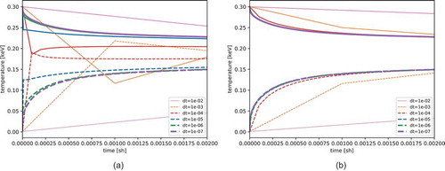
shows the temperature histories for this problem for the LMFG and fully converged nonlinear methods; all variations that fully converge the outer nonlinear loop get the same results. For large time steps, the LMFG method is not stable and shows violations of the maximum principle. This has been explored extensively in the context of Implicit Monte Carlo; see, for example, CitationRef. 12. The largest time step with a stable LMFG solution is sh, and it does not appear converged until at least
sh. On the other hand, fully converging the outer nonlinear iterations is always stable, if inaccurate. The solution appears converged at
sh, which is larger than where LMFG is stable.
Fig. 1. Temperature with two of the iteration methods. All of the fully converged nonlinear methods get the same solutions, so only one is shown. The stability limits of LMFG are clearly violated for large time steps. Solid lines are the radiation temperature, and dashed lines are the material temperature
For the solutions at sh and
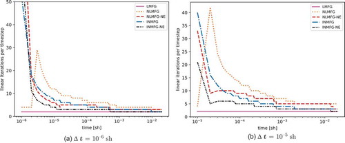
sh, we plot the total number of multigroup linear iterations in . Generally, the LMFG method is the cheapest by this metric, but that ignores the solution quality shown in . Fully converging both the outer Newton and inner linear system (NLMFG) is clearly the most expensive, which was also observed by Brown and WoodwardCitation1 and Lowrie.Citation2 Doing an inexact Newton step with only one inner linear multigroup solve also performs better. The nonlinear elimination variants NLMFG-NE and Inexact-Newton Multifrequency Grey with Nonlinear Elimination (INMFG-NE) performed better than the unaccelerated versions. Once the initial transient has passed, INMFG-NE has the same cost as LMFG. This is the true value of this method. It rapidly converges to the fully converged nonlinear solution when necessary, and it automatically transitions to an algorithm with the same cost as LMFG when the time steps are small enough for that method to work reasonably well.
Fig. 2. Linear iterations per time step, as measured by doing one solve for each of the diffusion equations in EquationEqs. (29)(29)
(29) , Equation(35)
(35)
(35) , and Equation(33)
(33)
(33)
shows the cumulative number of linear iterations for each method needed to get to the goal time of sh for the different time step sizes. By far the most effective way to reduce iterations and run time is to increase the time step size, as long as the solution is accurate. Also, note that INMFG-NE has the best performance for all the fully converged nonlinear solution methods, for the given discrete time and space system. In fact, even when LMFG is stable and producing reasonable results, INFMG-NE costs at most 40% more. Note that for
sh, LMFG gives unphysical solutions, so these low iteration counts are not meaningful.
TABLE II Cumulative Linear Iterations to Reach sh in the Infinite Medium Problem
V.B. Two-Dimensional Radiation Flow
We now test the methods on a multidimensional problem based on the one in CitationRef. 8 with one slight modification. Here, we will run in Cartesian X,Y coordinates while the original version used cylindrical R,Z coordinates.
shows the overall geometry together with sample solutions for the radiation and material temperatures. The problem is defined on a rectangle from and
. The mesh has uniform zone zones of
cm except in the
direction between
, where at
cm, the zone size was
cm. Each successive zone was
times bigger than the previous zone for a total of ten zones across this region.
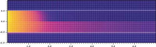
Fig. 3. Geometry of the two-dimensional radiation flow problem. There is a low-density material surrounded by a high-density material, with a symmetry plane at . The top half shows the material temperature at
sh, and the bottom half shows the radiation temperature at the same time but reflected about the
-axis. See for a more quantitative view of the temperatures
The material in the region cm has a density of
g/cm3, and for
cm, the density is
g/cm3. The specific heat is
jerk/g·keV. The opacity model coefficients are
,
, and
. There are ten radiation groups with group bounds in kilo-electron-volts of (
,
,
,
,
,
,
,
,
,
, and
).
Reflecting boundary conditions were applied on all boundaries, except on the left at cm and for
cm, where an isotropic incoming flux injected energy into the problem. For the reflecting boundaries, the coefficients in EquationEq. (12
(12)
(12) ) are
,
, and
. The incoming flux boundary source linearly increases from
keV to
keV over the range
sh and remains constant after the initial ramp. For the coefficients in EquationEq. (12
(12)
(12) ), this implies
,
, and
We tested the algorithms with three different time step sizes of sh,
sh, and
sh. The goal time is
sh, which is shorter than the goal time of
sh in CitationRef. 8. At
sh, the LMFG method is unstable and showed overheating in the material much like in the infinite medium problem. This can be seen in . All of the methods that fully converge the nonlinear system get the same, more physically realistic, solution. To more quantitatively demonstrate this, the radiation and material temperatures along the line
cm are shown at
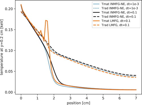
sh for several methods and time step sizes in . It is clear that the problem is not converged in time at the larger time step size, but the fully converged solutions are capturing the timescale of the Marshak wave traveling through the material reasonably well.
Fig. 4. Material temperature at sh. The unstable LMFG method is on top. All of the other methods that fully converge the nonlinear system produce the solution on the bottom
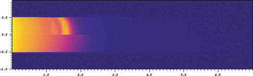
Fig. 5. The material and radiation temperatures in the pipe problem at sh along the line
cm. The solutions of LMFG and INMFG-NE are shown for
sh and of INMFG-NE for
sh
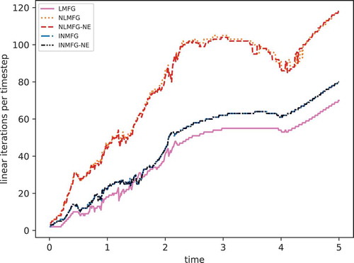
The per time step linear iteration counts are shown for the sh in . For this problem, we see again that the INMFG and INMFG-NE methods outperform the NLMFG and NLMFG-NE methods. The nonlinear elimination only marginally improves the convergence in this problem. The cumulative total number of iterations to reach the end time of
sh is shown in . This demonstrates that for a variety of time step sizes, INMFG-NE has marginally more cost than LMFG at increased stability and accuracy. In fact, given the particular tolerances selected, it appears that the first iteration of the nonlinear methods was just above the tolerance level; slightly loosening the tolerances would have made the nonlinear methods converge in just one iteration too. Fully converging both the inner and outer iteration loops in NLMFG and NLMFG-NE is dramatically more expensive, which mirrors the previous observations in CitationRefs. 1 and Citation2. Note that for
sh, LMFG gives unphysical solutions.
TABLE III Cumulative Linear Iterations to Reach sh in the Pipe Problem
Fig. 6. The number of linear iterations per time step for each of the different methods at sh. Note that the nonlinear elimination variants only marginally improve the unaccelerated methods for this problem, so the curves are nearly the same
VI. CONCLUSIONS AND FUTURE WORK
We recently discovered that we could apply the nonlinear elimination method in CitationRef. 13 to describe the algorithm in our discrete ordinates TRT code Teton. This has led to a mathematical framework for describing a family of accelerated nonlinear solution methods. By proper choices of tolerances at various levels of the new framework, we can recover the standard LMFG method in CitationRefs. 8 and Citation11, the (previously unpublished) algorithm in Teton that we call Inexact-Newton Multifrequency-Grey with Nonlinear Elimination (INMFG-NE), as well as several other algorithms.
The INFMG-NE method’s efficacy is due to three key algorithmic components. First, a standard grey acceleration step significantly speeds up convergence of the absorption and reemission of photons within a Newton iteration. Second, the new nonlinear elimination step effectively accelerates the emission and reabsorption within a Newton step. Because the emission is fundamentally nonlinear through the Planck function, it must be handled with a nonlinear method. Third, combining the grey acceleration and nonlinear elimination steps with an inexact Newton method allows only a single multigroup linear iteration per Newton step to be robust. All three in combination makes fully converging the nonlinear system practical.
In two test problems, we find (unsurprisingly) that fully converging the nonlinear system (with a given space and time discretization error) allows for larger time steps and better accuracy than the linearized one-step method LMFG. We also find that the traditional NLMFG method, which fully converges both the multigroup linear system for each Newton step and the outer nonlinear iterations, is prohibitively expensive. By combining the three acceleration techniques that make up INMFG-NE, we find that we can compute a fully converged nonlinear solution with very nearly the same cost as converging only the inner multigroup linear system in the LMFG method, particularly given that the increased robustness and accuracy of the fully converging nonlinear system allows for larger time steps. The INMFG-NE method seamlessly transitions from doing more iterations where needed for large nonlinear excursions to an algorithm with the cost of the LMFG method when the problem could be robustly linearized.
In the future, we plan to formally apply this method to the full Boltzmann transport equation, including inelastic Compton scattering. We are also excited to investigate the nonlinear preconditioning literatureCitation13–15 for additional methods that may be more effective for solving the thermal radiation transport equations.
Acknowledgments
Lawrence Livermore National Laboratory is operated by Lawrence Livermore National Security, LLC, for the U.S. Department of Energy, National Nuclear Security Administration under contract DE-AC52-07NA27344. This document was prepared as an account of work sponsored by an agency of the United States government. Neither the United States government nor Lawrence Livermore National Security, LLC, nor any of their employees makes any warranty, expressed or implied, or assumes any legal liability or responsibility for the accuracy, completeness, or usefulness of any information, apparatus, product, or process disclosed, or represents that its use would not infringe privately owned rights. Reference herein to any specific commercial product, process, or service by trade name, trademark, manufacturer, or otherwise does not necessarily constitute or imply its endorsement, recommendation, or favoring by the United States government or Lawrence Livermore National Security, LLC. The views and opinions of authors expressed herein do not necessarily state or reflect those of the United States government or Lawrence Livermore National Security, LLC, and shall not be used for advertising or product endorsement purposes. Document number: LLNL-JRNL-797841.
Notes
a Later, these will be the material and radiation balance equations.
b In methods that only do one Newton step, we often think of this as the absorption and reemission for the entire time step.
References
- P. BROWN and C. WOODWARD, “Preconditioning Strategies for Fully Implicit Radiation Diffusion with Material-Energy Transfer,” SIAM J. Sci. Comput., 23, 2, 499 (2001); https://doi.org/10.1137/S106482750037295X.
- R. B. LOWRIE, “A Comparison of Implicit Time Integration Methods for Nonlinear Relaxation and Diffusion,” J. Comput. Phys., 196, 2, 566 (2004); https://doi.org/10.1016/j.jcp.2003.11.016.
- P. NOWAK and M. NEMANIC, “Radiation Transport Calculations on Unstructured Grids Using a Spatially Decomposed and Threaded Algorithm,” Proc. Int. Conf. Mathematics and Computation, Reactor Physics and Environmental Analysis in Nuclear Applications, Madrid, Spain, September 27–30 1999.
- P. MAGINOT, P. NOWAK, and M. ADAMS, “A Review of the Upstream Corner Balance Spatial Discretization,” Proc. Int. Conf. Mathematics and Computational Methods Applied to Nuclear Science and Engineering, Jeju, Korea, April 16–20, 2017. LLNL-CONF-721617, Lawrence Livermore National Laboratory; https://www.osti.gov/biblio/1357379 ( current as of Nov. 19, 2019).
- J. I. CASTOR, Radiation Hydrodynamics, Cambridge University Press, Cambridge, United Kingdom (2004).
- P. G. MAGINOT and T. A. BRUNNER, “Lumping Techniques for Mixed Finite Element Diffusion Discretizations,” J. Comput. Theor. Transport., 47, 4–6, 301 (2018); https://doi.org/10.1080/23324309.2018.1461653.
- T. A. BRUNNER, “Preserving Positivity of Solutions to the Diffusion Equation for Higher-Order Finite Elements in Under Resolved Regions,” Proc. Mathematics & Computation (M&C+SNA+MC 2015), Nashville, Tennessee, April 19–23, 2015, American Nuclear Society (2015). LLNL-PROC-666744, Lawrence Livermore National Laboratory (2015); https://www.osti.gov/biblio/1182246 ( current as of Nov. 19, 2019).
- J. E. MOREL, T.-Y. B. YANG, and J. S. WARSA, “Linear Multifrequency-Grey Acceleration Recast for Preconditioned Krylov Iterations,” J. Comput. Phys., 227, 1, 244 (2007); https://doi.org/10.1016/j.jcp.2007.07.033.
- E. LARSEN, “A Grey Transport Acceleration Method Far [sic]Time-Dependent Radiative Transfer Problems,” J. Comput. Phys., 78, 2, 459 (1988); https://doi.org/10.1016/0021-9991(88)90060-5.
- J. FLECK and J. CUMMINGS, “An Implicit Monte Carlo Scheme for Calculating Time and Frequency Dependent Nonlinear Radiation Transport,” J. Comput. Phys., 8, 3, 313 (1971); https://doi.org/10.1016/0021-9991(71)90015-5.
- J. MOREL, E. LARSEN, and M. MATZEN, “A Synthetic Acceleration Scheme for Radiative Diffusion Calculations,” J. Quant. Spectrosc. Radiat. Transfer, 34, 3, 243 (1985); https://doi.org/10.1016/0022-4073(85)90005-6.
- S. W. MOSHER and J. D. DENSMORE, “Stability and Monotonicity Conditions for Linear, Grey, 0-D Implicit Monte Carlo Calculations,” Trans. Am. Nucl. Soc., 93, 1, 520 (2005).
- P. J. LANZKRON, D. J. ROSE, and J. T. WILKES, “An Analysis of Approximate Nonlinear Elimination,” SIAM J. Sci. Comput., 17, 2, 538 (1996); https://doi.org/10.1137/S106482759325154X.
- P. R. BRUNE et al., “Composing Scalable Nonlinear Algebraic Solvers,” SIAM Rev., 57, 4, 535 (2015); https://doi.org/10.1137/130936725.
- L. LIU and D. E. KEYES, “Field-Split Preconditioned Inexact Newton Algorithms,” SIAM J. Sci. Comput., 37, 3, A1388 (2015); https://doi.org/10.1137/140970379.
- A. T. TILL, J. S. WARSA, and J. E. MOREL, “Application of Linear Multifrequency-Grey Acceleration to Preconditioned Krylov Iterations for Thermal Radiation Transport,” J. Comput. Phys., 372, 931 (2018); https://doi.org/10.1016/j.jcp.2018.06.017.
- B. A. CLARK, “Computing Multigroup Radiation Integrals Using Polylogarithm-Based Methods,” J. Comput. Phys., 70, 2, 311 (1987); https://doi.org/10.1016/0021-9991(87)90185-9.
- T. A. DAVIS, “Algorithm 832: UMFPACK V4.3—An Unsymmetric-Pattern Multifrontal Method,” ACM Trans. Math. Softw., 30, 2, 196 (2004); https://doi.org/10.1145/992200.992206.