Real-Time Monitoring for Detection of Adversarial Subtle Process Variations

Abstract

As industries take advantage of the widely adopted digitalization of industrial control systems, concerns are heightened about their potential vulnerabilities to adversarial attacks. False data injection attack is one of the most realistic threats because the attack could be as simple as performing a reply attack allowing attackers to circumvent conventional anomaly detection methods. This attack scenario is real for critical systems, e.g., nuclear reactors, chemical plants, etc., because physics-based simulators for a wide range of critical systems can be found in the open market providing the means to generate physics-conforming attack. The state-of-the-art monitoring techniques have proven effective in detecting sudden variations from established recurring patterns, derived by model-based or data-driven techniques, considered to represent normal behavior. This paper further develops a new method designed to detect subtle variations expected with stealthy attacks that rely on intimate knowledge of the system. The method employs physics modeling and feature engineering to design mathematical features that can detect subtle deviations from normal process variation. This work extends the method to real-time analysis and employs a new denoising filter to ensure resiliency to noise, i.e., ability to distinguish subtle variations from normal process noise. The method applicability is exemplified using a hypothesized triangle attack, recently demonstrated to be extremely effective in bypassing detection by conventional monitoring techniques, applied to a representative nuclear reactor system model using the RELAP5 computer code.

Keywords:

• Model-based
• real-time online monitoring
• false data injection
• higher-order components

I. INTRODUCTION

Many industries are actively pursuing a digital transformation of their systems to realize the benefits of digitization, e.g., improved efficiency, optimized economy, and higher system visibility. Effectively, digitization is sought to improve system awareness of its own state and allow the system to optimally react to various process changes. However, this wave of digitization has introduced its own set of new vulnerabilities. Of interest here is cybervulnerability, manifesting in the form of adversarial intrusion into the system digital network for near-term or long-term malicious purposes, e.g., denial or interruption of service, degraded performance, etc. The increased frequency and sophistication of recent cyberattacks against cyberphysical systems make it clear that reliable defenses must be established to ensure zero impact on the system function while under attack.

The initial response to these threats has focused on the adoption of information technology (IT) defenses aiming to stop unauthorized access via firewalls, passcodes, virtual private networks (VPNs), etc. With the ever-increasing sophistication in hacking methods, recent attacks have proven that IT defenses can be eventually bypassed by determined adversaries, e.g., state-sponsored or criminal organizations. Among the most famous attacks is the state-sponsored Stuxnet malware that compromised the control network of the Natanz Iranian enrichment plant leading to its shutdown after damaging thousands of its centrifuges.¹ Other similar daring attacks occurred thereafter, e.g., attacks against the Japanese Monju nuclear power plant,² the Gundremmingen nuclear power plant in Germany,³ the electric grid in Ukraine,⁴ and the nuclear industry in India,⁵ as well as a hack in Florida against a water distribution center.⁶

In light of these threats, it has become critical to build another layer of defense when IT defenses are compromised. This new layer is referred to as operational technology (OT) defense. Operational technology defenses focus on the physical process as described by network data comprising sensor readings, process variables, and actuating commands. The OT defenses ask this question: Are the engineering network data consistent with expected behavior? In a sophisticated false data injection (FDI) attack, the attacker relies first on delivering an IT payload, designed to penetrate through the IT defenses. This represents the conventional first step for any hacking attempt, i.e., gaining access to the system. Following that, the attacker must deliver another payload, referred to as the engineering payload. This payload is designed to cause the system to move along an undesirable trajectory.⁷

These maneuvers can be achieved in multiple ways. For example, the engineering payload could falsify the sensor data, causing the control algorithms to send signals to the actuators that cause undesirable performance. Another approach is to change the control algorithm logic to achieve similar goals. In all scenarios, the payload must be aware of the normal engineering checks that exist in the network. These checks are developed by the engineering team to ensure that the system is reliably responding to normal process variations. Thus, unlike IT defenses, which rely on the use of generic methods to protect access to the information, OT defenses must be cognizant of the engineering design and safety procedures in place. To achieve that, OT defenses must rely on an online monitoring approach to continuously check the engineering data, i.e., sensor readings, process variables, and actuator commands, and be able to determine whether the data are real, i.e., have originated from the system, or are falsified, i.e., have been potentially tampered with.

This distinction between IT and OT defenses underpins the key challenge for designing OT defenses. For IT defenses, the goal is to block access regardless of the engineering values of the process variables, implying that one simply needs to adopt a fortress defense mentality. It does not matter what one protects; the only thing that matters is how to build an incredible barrier that is difficult to bypass. For OT defenses, however, the goal is to determine whether the variables of the system process variables (an inevitable occurrence in any real industrial process) are naturally occurring or maliciously introduced. The implication is that the defense must depend on a predetermined specification of what is normal and what is abnormal. Further, given the proliferation of critical systems worldwide, representing the key components of any country’s critical infrastructure, the OT defenses must assume that the attacker will likely recruit subject matter experts capable of differentiating between normal and abnormal behavior.

There are two general approaches to achieve this monitoring for OT purposes: passive and active. Passive monitoring implies observing the system for a period of time to understand, i.e., establish a basis to describe, its normal behavior and use this understanding to judge whether the system behavior at a later time has deviated from its expected normal behavior.⁸ Active monitoring relies on injecting perturbations into the engineering data to ensure their trustworthiness.^9,10 Effectively, active monitoring may be thought of as inserting secret messages in the data to determine when the data are being tampered with.

The logic behind passive monitoring is that one needs to observe to develop an understanding while active monitoring argues that one needs to interfere to develop an even better understanding. Both viewpoints have their merits and challenges. For example, a key challenge of passive monitoring is that the attacker is expected to do the same thing done by the defender, i.e., observe the network during a lie-in-wait period before introducing changes to the process variables and sensors data. The more familiarity the attacker has with the system, the easier it is to build an understanding of its behavior, ultimately reaching the level of understanding of the OT defense designer. In active monitoring, the first challenge is to ensure that the injected perturbations do not penalize the system function. Second, if the secret perturbations follow a pattern that can be detected using passive monitoring, the whole purpose of inserting perturbations is defeated because the attacker can learn their patterns and ultimately circumvent them. Clearly, both of these challenges require a good understanding of system behavior, achieved via passive monitoring.

One of our previous papers⁸ provides a detailed explanation of the challenges and limitations of passive monitoring. This previous paper argues that while passive monitoring may be the preferred mode for detection, it cannot solely guarantee an effective OT defense when the attacker has privileged access to the system models and design details, expected to be the case with an insider attack. Hence, a strategy that involves both passive and active monitoring ought to be pursued. Methods to circumvent the challenges of active monitoring are discussed in another paper.^11,12

The current paper focuses entirely on passive monitoring. Particularly, the proposed method aims to address the following challenge: How can a defender develop an understanding of system behavior that is difficult to duplicate by an attacker, who is also expected to rely on passive monitoring to learn system behavior? A key assumption made here is that the attacker does not have an exact replica of the physics model employed by the defender. This is not an unrealistic assumption; however, it recognizes that the attacker is expected to have access to models that are sufficiently similar to the defender’s models. This is due to their familiarity with the system. For nuclear reactors, representing the focus of our application, this is an expected scenario because the modeling of nuclear reactors is well understood, implying that different models of sufficient similarity could be developed to describe the same system.

Passive monitoring OT defenses adopt two general approaches: data-driven approaches or model-based approaches. Data-driven approaches rely on the use of data mining techniques to establish patterns in the engineering data based on past behavior. An adversary trying to change the engineering data, e.g., process variables and sensor data, unaware of these patterns, will introduce changes that can be detected when deviating from the patterns. Model-based approaches require building a faithful mathematical model that describes the behavior of the system. When the measurements deviate from the predictions, alarms may be issued. Next, we overview some of the methods employing both data-driven and model-based techniques from the literature.

Eggers employs principal component analysis (PCA), independent component analysis (ICA), and their variants to detect FDI attack intrusion under different scenarios. Egger’s work indicates that static ICA and PCA may not be sufficient, but a moving window version of PCA and ICA can quantitively identify the onset of the attacks.¹³ Eggers’s work has primarily focused on FDI attacks that introduce noticeable changes to the engineering data, e.g., a sudden drop, patterned sensor drifts, or flat-lining of process variables. Zhang and Coble employ auto-associative kernel regression to determine whether sensor data are authentic by using the idea of sensor virtualization, wherein a group of sensors is employed to predict the reading of a given suspect sensor. The residual between the measured and predicted values serves as a measure of security status; i.e., if the residuals go beyond the predefined threshold, a support vector regression–based inference model is employed to calculate the countermeasure commands sent to actuators.¹⁴ Wang et al. apply a nonparametric cumulative sum approach to the Advanced Lead-cooled Fast Reactor European Demonstrator (ALFRED) for online monitoring of cyberattacks to a multiloop controller.¹⁵ In Wang’s work, the detection is fulfilled by a score function that will not exceed the prespecified threshold under normal operation. Gawand et al. employ least-squares approximation followed with a convex hull approach to determine the authenticity of the measurement.¹⁶ This is effective for FDI attacks that manifest as random bias. Zhao et al. employ a semi-Markov decision process to model the interactions between the defender and the attacker, in which each state is quantified as a state value, referred to as rewards, and the best choice for both defenders and attackers is calculated by the optimal rewards.¹⁷ This study provides a guide for defenders’ optimal response to cyberattacks under various situations. Similarly, Vaddi et al. employ the dynamic Bayesian network for inferring the hidden state of the system from the observed variables by probabilistic theory.¹⁸ Both works are built based on the state transition probability derived from probability risk analysis, indicating that the success and credibility of the whole model highly depend on the reliability of this prior knowledge. For employing the model-derived correlations, Li and Huang employ dynamic PCA to characterize the correlation between multiple variables and consequently use a chi-square detector to distinguish adversarial cyberattacks from ordinary random failures.¹⁹

These aforementioned methods, developed in different disciplines, share one thing in common: They rely on capturing the dominant behavior from operational data or correlation between process variables, mathematically referred to as active degrees of freedom (DOFs) or lower-order components (LOCs), to make predictions. For example, PCA relies on singular value decomposition (SVD) to compute the principal components, representing the few right or left singular vectors, hereinafter referred to as the LOCs.

For illustration, Fig. 1 shows the components of typical sensor variations as projected onto the components identified by PCA. The x-axis represents the index of the components, and the y-axis shows the significance of the components. The components in the blue box represent the LOCs, expected to be known by the attackers, which can be captured by data-driven techniques or an approximate physics model.²⁰ This implies that once the LOCs are learned during the initial lie-in-wait period, the attackers would be able to falsify the measurements respecting the dominant patterns of system behavior. With that, they would be able to bypass detection by techniques relying solely on capturing the dominant behavior.²¹ However, the LOCs remain an effective signature for patterns that significantly deviate from normal behavior such as (1) constant bias, (2) measurement drift with function of time, (3) wider noise, (4) dynamic process variable freezing as a constant, etc. However, if the attackers attempt to falsify the data using the LOCs, the majority of FDI techniques described earlier would be potentially bypassed.

Fig. 1. Dominance ordering of extracted process patterns.

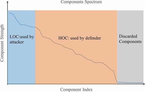
To detect these stealthy attack scenarios, one needs to rely on capturing more features that capture the less dominant patterns of system behavior, hereinafter denoted as higher-order components (HOCs), as shown in the orange box in Fig. 1. Unlike the LOCs, which can be seamlessly captured using approximate models, the HOCs are much more sensitive to the system characteristics, e.g., past behavior, modeling assumptions, etc. If the attacker has the same exact model as the defender, then, ultimately, the proposed approach may also be bypassed. As mentioned earlier, this extreme scenario should be handled using active monitoring, which is outside the scope of this work. Instead, it is assumed that the attackers are equipped with a sufficiently accurate model; however, it does not faithfully duplicate the defender’s model, which is often carefully calibrated to operational data. As we will show later, the HOCs allow the defender to take advantage of the subtle variations between the attackers’ and the defenders’ models, allowing defenders to detect FDI attacks that respect the patterns established by the LOCs. The idea is to derive features that are based on both the LOCs and the HOCs as a basis for classifying normal data from FDI behavior masquerading as normal behavior.

Our earlier work, which proposes the use of randomized window decomposition (RWD) to identify LOC-based and HOC-based features,⁸ has demonstrated the potential of this OT defense for an idealized scenario, where the data are assumed to be available off-line. In this paper, we demonstrate how RWD can be used to detect subtle data falsifications in real time with interference from normal process noise. Particularly, we analyze a stealthy attack called triangle attack,⁷ which employs a series of line segments to respect the system dynamic behavior without prior knowledge of the system dynamical model. The RWD algorithm is adapted for real time and is equipped with a denoising algorithm to ensure noise does not interfere with the HOCs.

II. METHODOLOGY

The proposed OT defense relies solely on passive monitoring and comprises two procedures: a denoising procedure employing a recently developed multilevel denoising algorithm and a feature extraction procedure employing the RWD algorithms. Section II.A introduces the denoising algorithms starting from a single-level smoothing strategy and extending to the employed multilevel smoothing strategy. Section II.B discusses the feature extraction procedure when monitoring a single process variable, referred to as univariate monitoring, followed by an extension to multivariate monitoring in Sec. II.C. Sections II.D and II.E evaluate the proposed attack detection algorithms by the time delay criterion and limits of distance, respectively.

II.A. Single-Level and Multilevel Denoising Algorithms

The evolution of a process variable, representing a state variable, a model output response, a sensor reading, etc., is described as a time series, denoted as ϕ(t). Following the principles of mathematical decomposition, ϕ(t) can be expressed as a linear combination of a number of basis functions, as shown in Eq. (1)(1) $\varphi \left(t\right)\approx \sum _{j=1}^r{\alpha }_j{\phi }_j\left(t\right),$(1) :

(1) $\varphi \left(t\right)\approx \sum _{j=1}^r{\alpha }_j{\phi }_j\left(t\right),$(1)

where the left side often represents the function ϕ(t) over a given observation (or signature) window and ${\phi }_j\left(t\right)$ represents the associated basis functions. The coefficient α_j represents the projection of ϕ(t) onto ${\phi }_j\left(t\right):$

(2) ${\alpha }_j={\phi }_j^T(t)\varphi \left(t\right).$(2)

This decomposition is sought because in many realistic scenarios, one can show that for many complex systems, ϕ(t) may be expressed using a few r basis functions. Unlike Taylor series or Fourier expansion, where the basis functions are predetermined resulting in r being very large, recent research in reduced-order modeling has shown that with a careful choice of the basis functions, one can generate function approximations that are acceptably accurate with only a low number of terms.^22,23 Most of these techniques rely on the use of nonparametric techniques like PCA or SVD that minimize the reduction error of the form:

(3) $e_r=\underset{{\phi }_j}{min}{∥\varphi \left(t\right)-\sum _{j=1}^r{\alpha }_j{\phi }_j\left(t\right)∥}^2.$(3)

Each one of the basis functions is referred to as an active DOF and collectively referred to as the active subspace. The active DOFs are indexed from being most to least dominant, with the dominance measuring their contribution to the original function; i.e., the first active DOF is the most dominant such that variations in its associated coefficient α_j result in the most function variation in ϕ(t).

For monitoring applications, ϕ(t) is formed as a series of discrete time measurements, here denoted as a one-dimensional column vector with length n, mathematically expressed in Eq. (4)(4) $\begin{array}{r}\varphi \left(t\right)=\mathbf{y}=\left(y_1,y_2,\cdots ,y_i,\cdots ,y_n\right),i=1,2,\cdots ,n,\end{array}$(4) :

(4) $\begin{array}{r}\varphi \left(t\right)=\mathbf{y}=\left(y_1,y_2,\cdots ,y_i,\cdots ,y_n\right),i=1,2,\cdots ,n,\end{array}$(4)

where y_i represents the measurement at the i’th time step. It is assumed that the analyst has access to many snapshots of a series of temporal evolution for reference, or normal function variations, obtained either from repeated model execution that simulates a plethora of normal operating conditions or from historical data, denoted here as

(5) ${\varphi }^{\mathrm{R}\mathrm{e}\mathrm{f}}\left(t\right)={\mathbf{y}}^{\mathrm{R}\mathrm{e}\mathrm{f}}=\left[y_1^{\mathrm{R}\mathrm{e}\mathrm{f}},y_2^{\mathrm{R}\mathrm{e}\mathrm{f}},\cdots ,y_i^{\mathrm{R}\mathrm{e}\mathrm{f}},\cdots ,y_n^{\mathrm{R}\mathrm{e}\mathrm{f}}\right].$(5)

These profiles are first normalized by their time-averaged values. No distinction between the normalized and the original values will be made to avoid cluttering the notations.

Next, we rely on a window-based approach for monitoring, where a user-defined signature window of size w is used to capture w-length snapshots of the vector of length n in Eq. (5)(5) ${\varphi }^{\mathrm{R}\mathrm{e}\mathrm{f}}\left(t\right)={\mathbf{y}}^{\mathrm{R}\mathrm{e}\mathrm{f}}=\left[y_1^{\mathrm{R}\mathrm{e}\mathrm{f}},y_2^{\mathrm{R}\mathrm{e}\mathrm{f}},\cdots ,y_i^{\mathrm{R}\mathrm{e}\mathrm{f}},\cdots ,y_n^{\mathrm{R}\mathrm{e}\mathrm{f}}\right].$(5) . If sequential snapshots are taken, the vector in Eq. (5)(5) ${\varphi }^{\mathrm{R}\mathrm{e}\mathrm{f}}\left(t\right)={\mathbf{y}}^{\mathrm{R}\mathrm{e}\mathrm{f}}=\left[y_1^{\mathrm{R}\mathrm{e}\mathrm{f}},y_2^{\mathrm{R}\mathrm{e}\mathrm{f}},\cdots ,y_i^{\mathrm{R}\mathrm{e}\mathrm{f}},\cdots ,y_n^{\mathrm{R}\mathrm{e}\mathrm{f}}\right].$(5) is turned into a rectangular Hankel matrix²⁴ H^Ref of size w × (n − w + 1):

(6) ${\mathbf{H}}^{\mathrm{R}\mathrm{e}\mathrm{f}}=\left[\begin{array}{cccc}{\mathbf{h}}_1^{\mathrm{R}\mathrm{e}\mathrm{f}}& {\mathbf{h}}_2^{\mathrm{R}\mathrm{e}\mathrm{f}}& \cdots & {\mathbf{h}}_{n-w+1}^{\mathrm{R}\mathrm{e}\mathrm{f}}\end{array}\right]=\left[\begin{array}{cccc}{y}_1^{\mathrm{R}\mathrm{e}\mathrm{f}}& y_2^{\mathrm{R}\mathrm{e}\mathrm{f}}& \cdots & y_{n-w+1}^{\mathrm{R}\mathrm{e}\mathrm{f}}\\ y_2^{\mathrm{R}\mathrm{e}\mathrm{f}}& y_3^{\mathrm{R}\mathrm{e}\mathrm{f}}& \cdots & y_{n-w+2}^{\mathrm{R}\mathrm{e}\mathrm{f}}\\ ⋮& ⋮& \ddots & ⋮\\ y_w^{\mathrm{R}\mathrm{e}\mathrm{f}}& y_{w+1}^{\mathrm{R}\mathrm{e}\mathrm{f}}& \cdots & y_n^{\mathrm{R}\mathrm{e}\mathrm{f}}\end{array}\right].$(6)

Mathematically, the SVD-based reduction of H may be described as follows:

(7) ${\mathbf{H}}^{\mathrm{R}\mathrm{e}\mathrm{f}}\mathbf{=}\mathbf{U}\mathbf{S}{\mathbf{V}}^T\approx \sum _{k=1}^r{s}_k{\mathbf{u}}_k{\mathbf{v}}_k^T,$(7)

where

$\mathbf{U}$ =	=	$\left({\mathbf{u}}_1,{\mathbf{u}}_2,\cdots ,{\mathbf{u}}_r\right)$
$\mathbf{S}$ =	=	$\mathrm{d}\mathrm{i}\mathrm{a}\mathrm{g}\left\{s_1,s_2,\cdots ,s_r\right\}$
$\mathbf{V}$ =	=	$\left({\mathbf{v}}_1,{\mathbf{v}}_2,\cdots ,{\mathbf{v}}_r\right)$
$r$ =	=	rank of the Hankel matrix.

The column vectors in the U matrix form a set of orthonormal bases for the column space spanned by ${\mathbf{h}}_k^{\mathrm{R}\mathrm{e}\mathrm{f}},k=1,2,\cdots ,r.$ The row vectors in V^T form a set of orthogonal bases for the row space spanned by the rows of ${\mathbf{H}}^{\mathrm{R}\mathrm{e}\mathrm{f}}.$ The S is a diagonal matrix storing the singular values in a descending order. The rank of the matrix r is usually determined by a user-defined tolerance, as expressed in Eq. (3)(3) $e_r=\underset{{\phi }_j}{min}{∥\varphi \left(t\right)-\sum _{j=1}^r{\alpha }_j{\phi }_j\left(t\right)∥}^2.$(3) . The active subspace basis functions ${\phi }_i\left(t\right)$ are expressed by the column vectors of the U matrix, i.e., ${\phi }_j\left(t\right)={\mathbf{u}}_j$.

Denote a normalized temporal evolution from raw sensor readings (with noise) of the process variables as $\mathbf{y}=\left(y_1,y_2,\cdots ,y_i,\cdots ,y_n\right),i=1,2,\cdots ,n,$ and the corresponding Hankel matrix at the i’th time step is denoted as ${\mathbf{H}}_i=\left[\begin{array}{cccc}{\mathbf{h}}_{i-w+1}& {\mathbf{h}}_{i-w+2}& \cdots & {\mathbf{h}}_i\end{array}\right]$, with w taken as the window size. The denoised measurements with single-level reduction are achieved via

$\begin{array}{rl}& {\hat{\mathbf{h}}}_{i-w+1}={\mathbf{U}\mathbf{U}}^T{\mathbf{h}}_{i-w+1}\\ & {\stackrel{\mathbf{ˆ}}{\mathbf{h}}}_{i-w+2}={\mathbf{U}\mathbf{U}}^T{\mathbf{h}}_{i-w+2}\\ & ⋮\\ & {\stackrel{\mathbf{ˆ}}{\mathbf{h}}}_i={\mathbf{U}\mathbf{U}}^T{\mathbf{h}}_i.\end{array}$

(8)

Therefore, the corresponding denoised Hankel matrix is expressed as

(9) ${\stackrel{\mathbf{ˆ}}{\mathbf{H}}}_i=\left[{\stackrel{\mathbf{ˆ}}{\mathbf{h}}}_{i-w+1},{\stackrel{\mathbf{ˆ}}{\mathbf{h}}}_{i-w+2},\cdots {\stackrel{\mathbf{ˆ}}{\mathbf{h}}}_i\right]={\mathbf{U}\mathbf{U}}^T{\mathbf{H}}_i.$(9)

Since one data point can be smoothed a maximum of w times, a given point y_i is no longer smoothed after i + w − 1 time steps. The final smoothed value ŷ_i is obtained by the first entry of ${\hat{\mathbf{H}}}_i$.

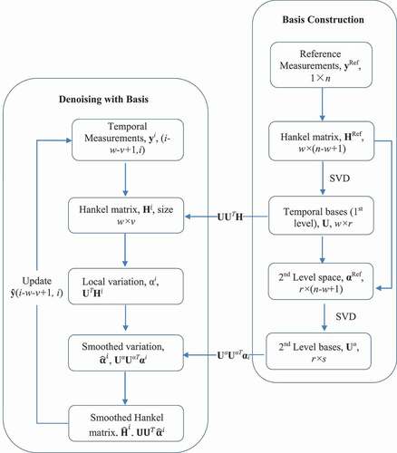
A multilevel smoothing can be thought of as simply extending the range of the smoothing function. Here, a two-level denoising is described to demonstrate the idea of multilevel denoising. Adopting the same notation in the single-level denoising, the final smoothed point ŷ_i would be iteratively denoised from the (i − w − v)’th time step to (i + w + v − 1)’th, where v denotes the window size of the second level of denoising. This indicates that one will get a final denoised ŷ_i after (w + v − 1) time steps.

The basic idea of the multilevel approach is to find sets of bases for each layer of denoising, the first of which is obtained as the U matrix in Eq. (7)(7) ${\mathbf{H}}^{\mathrm{R}\mathrm{e}\mathrm{f}}\mathbf{=}\mathbf{U}\mathbf{S}{\mathbf{V}}^T\approx \sum _{k=1}^r{s}_k{\mathbf{u}}_k{\mathbf{v}}_k^T,$(7) . Then, one needs to identify the bases for the second-level variations that are stored in the projection matrix ${\alpha }^{\mathrm{R}\mathrm{e}\mathrm{f}}$:

(10) ${\alpha }^{\mathrm{R}\mathrm{e}\mathrm{f}}={\mathbf{U}}^{\alpha T}{\mathbf{H}}^{\mathrm{R}\mathrm{e}\mathrm{f}}.$(10)

Similarly, SVD is adopted to identify the basis of the second-level variations, as shown in Eq. (11)(11) ${\alpha }^{\mathrm{R}\mathrm{e}\mathrm{f}}={\mathbf{U}}^{\alpha }{\mathbf{S}}^{\alpha }{\mathbf{V}}^{\alpha T}\approx \sum _{k=1}^s{s}_k^{\alpha }{\mathbf{u}}_k^{\alpha }{\mathbf{v}}_k^{\alpha T},$(11) :

(11) ${\alpha }^{\mathrm{R}\mathrm{e}\mathrm{f}}={\mathbf{U}}^{\alpha }{\mathbf{S}}^{\alpha }{\mathbf{V}}^{\alpha T}\approx \sum _{k=1}^s{s}_k^{\alpha }{\mathbf{u}}_k^{\alpha }{\mathbf{v}}_k^{\alpha T},$(11)

where the superscript α represents the second-level mapped variation related quantities/matrix and the rank of the second-level variation spanned subspace is denoted as s. To capture the main variation of the process variable’s components, one needs to project the temporal measurements onto the U matrix to capture most dominant variations for current measurements, as mathematically expressed in Eq. (12)(12) ${\alpha }^i={\mathbf{U}}^T{\mathbf{H}}^i.$(12) :

(12) ${\alpha }^i={\mathbf{U}}^T{\mathbf{H}}^i.$(12)

Speaking in the context of online monitoring, a dynamic Hankel matrix Hⁱ is constructed with the window size for the second-level components, where the superscript i of Hⁱ represents the index of the data points. The multilevel denoising works as the inner iteration for the high-level variation mapped matrices. Here, the denoised second-level variation is expressed as

(13) ${\stackrel{\mathbf{ˆ}}{\alpha }}^i={\mathbf{U}}^{\alpha }{\mathbf{U}}^{\alpha T}{\alpha }^i.$(13)

With the denoised high-level variations, the low-level variations can be recovered by being mapped back to the basis at the corresponding level, as shown in Eq. (14)(14) ${\stackrel{\mathbf{ˆ}}{\mathbf{H}}}^i={\mathbf{U}\mathbf{U}}^T{\stackrel{\mathbf{ˆ}}{\alpha }}^i.$(14) :

(14) ${\stackrel{\mathbf{ˆ}}{\mathbf{H}}}^i={\mathbf{U}\mathbf{U}}^T{\stackrel{\mathbf{ˆ}}{\alpha }}^i.$(14)

Therefore, the multilevel smoothed Hankel matrix can be expressed in Eq. (15)(15) ${\stackrel{\mathbf{ˆ}}{\mathbf{H}}}^i={\mathbf{U}\mathbf{U}}^{\alpha }{\mathbf{U}}^{\alpha T}{\mathbf{U}}^T{\mathbf{H}}^i.$(15) :

(15) ${\stackrel{\mathbf{ˆ}}{\mathbf{H}}}^i={\mathbf{U}\mathbf{U}}^{\alpha }{\mathbf{U}}^{\alpha T}{\mathbf{U}}^T{\mathbf{H}}^i.$(15)

For illustration, this overall denoising calculation scheme is depicted in Fig. 2.

Fig. 2. Multilevel denoising calculational scheme.

Following the basic idea of multilevel denoising, the single-level denoising algorithm can be seamlessly extended to employ the basis from higher level, which can be expressed as

(16) ${\stackrel{\mathbf{ˆ}}{\mathbf{H}}}^i={\mathbf{U}}_1{\mathbf{U}}_2{\mathbf{U}}_3\cdots {\mathbf{U}}_m{\mathbf{U}}_m^T\cdots {\mathbf{U}}_3^T{\mathbf{U}}_2^T{\mathbf{U}}_1^T{\mathbf{H}}^i,$(16)

where m represents the total number of layers adopted for denoising. Also, the final smoothed ŷⁱ will be obtained after T time steps, expressed in Eq. (17)(17) $T=\sum _{l=1}^m{w}_l-1,$(17) :

(17) $T=\sum _{l=1}^m{w}_l-1,$(17)

where w_l represents the window size at layer l. In other words, for online monitoring, the time delay resulting from denoising is T. The total number of layers m will not increase to infinity since the information at each layer decreases as the number of layers increases. In addition, the increased number of layers will lead to an increasing of time delay. Thus, one needs to conduct a series of tests for proper selection of the number of layers and rank identification of each layer such that one can achieve an optimal trade-off between retrieved information and the delay from denoising. The effectiveness of the denoising approach is demonstrated in another paper.²⁵

II.B. Univariate Monitoring for FDI Attack Detection

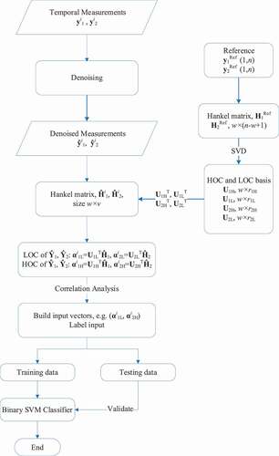
For online real-time FDI detection, one needs to construct features representing the dominant, i.e., LOCs, and nondominant, i.e., HOCs, behaviors of the system such that a classifier can distinguish subtle data falsification. Adopting the same set of notations as in Sec. II.A, the steps of the univariate FDI attack detection algorithm for online monitoring are stated below. Details of this algorithm were previously published in Ref. 8 and are reproduced here briefly for the sake of complete discussion. The algorithm relies on the idea of generating hypothetical attack scenarios to allow for a supervised learning–based support vector machine (SVM) classifier. Supervised learning is the preferred approach for binary classification; however, in practice, it is impossible to come up with all the possible scenarios that are representative of adversarial attacks.

To overcome this challenge, we employ an approach in which the defender first generates the LOC and HOC features, as derived from genuine data. Genuine data, hereinafter denoted by the subscript g, may be collected from a simulator, i.e., using a model-based approach, or can be directly gleaned from sensor data, i.e., using a data-driven approach. The genuine data are then modified using piecewise line segments to represent the attack data, denoted below with the subscript a. The attack scenario considered in this work is one in which the attacks aim to alter the process while feeding falsified data to the operator. These falsified data are generated using either physics-based or data-driven models, both expected to emulate the behavior of the system. With the proposed algorithm, the goal is to detect that the falsified data are not genuine; hence, an intrusion alarm can be raised. The idea here is that the evolution of any adversarial attack may be decomposed into a number of these line segments; i.e., they serve as an effective decomposition basis for any FDI attack. These line segments are placed randomly over all the genuine data profiles and are fed to the SVM binary classifier as attack data. An important outcome of this approach is that it will allow the analyst to determine the minimum threshold for detecting subtle variations under the presence of process noise, as will be shown in Sec. IV.

The details of the SVM classifier are presented as follows:

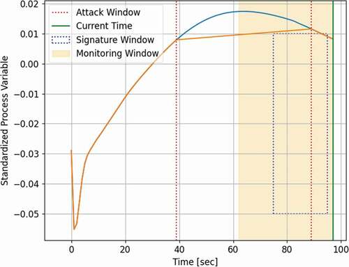
1. Employing a signature window of size w, sequentially place this window over the denoised genuine signal ${\stackrel{\mathbf{ˆ}}{\mathbf{y}}}^g=\left(y_{i-w-v+1}^g,\cdots ,y_i^g\right),i=w+v,w+v+1,\cdots ,n$, within the monitoring window, to generate v random snapshots for the window values, and aggregate in a matrix Hⁱ (w × v). Figure 3 illustrates the sliding signature window within the monitoring window.

2. Based on the defined tolerance, determine the rank, i.e., the number of components, denoted as r_L and r_H for the LOCs and the HOCs, respectively. The LOCs and the HOCs are captured in two matrices: U_L (w × r_L) and U_H (w × r_H).

3. Calculate the projection of each of the v signature windows from the Hⁱ matrix along the r_L LOCs and the r_H HOCs as features, and aggregate the features in two matrices of sizes r_H × v and r_L × v, denoted as ${\alpha }_H^g$ and ${\alpha }_L^g,$ respectively.

4. Repeat steps 1, 2, and 3 for the attack signals ${\stackrel{\mathbf{ˆ}}{\mathbf{y}}}^a=\left(y_{i-w-v+1},\cdots ,y_i\right),$ $i=w+v,w+v+1,\cdots ,n$ to generate matrices ${\alpha }_H^a$ and ${\alpha }_L^a$, in order to detect attacks injected during the period from time step i − w − v + 1 to time step i. The attack signals are generated by placing windows randomly throughout the genuine data and replacing the values by linear piecewise trends. Details on this may be found in a previous publication⁸ and in Sec. IV.

5. Prepare input datasets as a vector via the concatenation of the LOCs and the HOCs.

6. Use ‘0’ to label the feature column vectors in ${\alpha }_H^g$, ${\alpha }_L^g$, ${\alpha }_H^a,$ and ${\alpha }_L^a$ that do not contain falsified data, and use ‘1’ to label the other ones that contain attack data.

7. Train a binary SVM classifier to identify the feature vectors constructed from attack data.

Fig. 3. Illustration for sliding signature window.

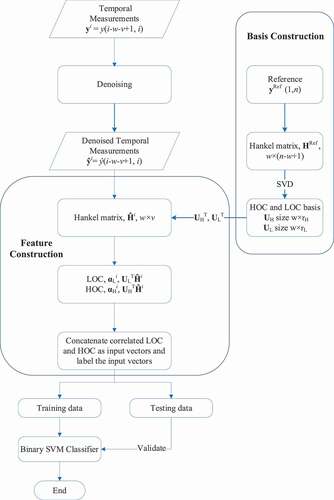
For illustration, the calculational scheme of the algorithm is shown in Fig. 4.

Fig. 4. Univariate calculational scheme of detection algorithm.

II.C. Multivariate Monitoring for FDI Attack Detection

Besides employing LOCs and HOCs from one process variable, another option is to construct features from different process variables, especially the ones that are expected to be correlated. This allows detection of attack scenarios in which the attacker has access to some of the historical sensor data, allowing a reply attack to be performed. To simulate this, we assume that some of the responses are duplicated from historical data and the rest are falsified by the attacker. We show that the combined use of LOCs and HOCs allows for the detection of this attack scenario.

The major difference from the univariate monitoring algorithm is that the multivariate monitoring algorithm fuses the feature vectors from multiple process variables. However, arbitrarily stacking of components may unnecessarily extend the feature vectors and weaken the classifier performance or add calculational burden to the classifier.

To mitigate these issues, a prior analysis of the components of different variables is conducted to determine which components should be used in feature construction. Taking two process variables as an example, with a user-defined tolerance, one can obtain the number of active DOFs for both variables, denoted as r₁ and r₂, and then build an r₁ × r₂ correlation matrix, from which one can identify the component pairs with least uncertainty. The identified pairs are then employed as the best candidates to construct feature vectors. For illustration, Fig. 5 shows the calculation scheme of the multivariate monitoring algorithm, where the subscripts 1 and 2 represent different process variables.

Fig. 5. Multivariate calculational scheme of detection algorithm.

II.D. Evaluation of Attack Detection

This section defines a detection criterion based on the results of the SVM classifier. The raw SVM results provide information on how often the classifier is triggered. To quantify that, over the temporal horizon, two metrics are defined: genuine coverage (GC) and attack coverage (AC). The GC metric measures the number of times the classifier returns a label of ‘0’ to denote genuine behavior, and the AC metric measures the number of times the classifier returns a label of ‘1’ to denote attack behavior. In ideal settings, the classifier is expected to be triggered when the monitoring window overlaps the attack window.

As would be expected, if the overlap is small, the likelihood of the classifier being triggered will be lower than if the overlap is large. To minimize the rate of false positives, a criterion should be developed in terms of the AC and GC metrics. Both metrics are normalized by the total number of time steps in which the monitoring window has overlap with the attack window. For example, for an attack window of 50 s, a monitoring window of 25 s, and a signature window of 20 s, there should be a total of 74 s in which the two windows overlap. Recall that the monitoring window is advancing 1 s at a time. Thus, a 20% AC implies that the classifier triggered a ‘1’ label for 20% of the 74 s. These two metrics are used to determine a criterion for detection as follows. An attack is declared when the classifier triggers a ‘1’ label five times in a row. This basic criterion is used in this work; however, more complicated criteria may be used that take into account the score of each label, which is a function of the distance from the decision boundary of the classifier. Some of these ideas will be explored in future work.

In addition to the binary decision of attacking detection, it is important to determine the time delay between the onset of the attack and its detection. Hence, a time delay t_d is defined in the context of real-time monitoring in Eq. (18)(18) $t_d=t_p-t_a,$(18) :

(18) $t_d=t_p-t_a,$(18)

where t_p refers to the time step at which the classifier is triggered when the classifier declares positive predictions that last t time steps and t_a refers to when the attack is injected. Ideally, one would want the detection time delay to approach zero.

II.E. Detection Limit Exploration

This paper focuses on the detection of subtle data falsification for online monitoring of nuclear systems, which raises the following question: How subtle can an attack be and still be detected? To explore this limit, a distance metric is defined measuring the discrepancy between the genuine and attack values over the attack window. This distance is defined in Eq. (19)(19) $d_l=\sqrt{\frac{\sum _{l=1}^{w_a}{(y_l^g-y_l^a)}^2}{w_a}},$(19) :

(19) $d_l=\sqrt{\frac{\sum _{l=1}^{w_a}{(y_l^g-y_l^a)}^2}{w_a}},$(19)

where

$y_l^g,$ $y_l^a$ =	=	normalized raw genuine and attack response values at l’th time step, respectively
$w_a$ =	=	size of the attack window.

Our goal is to find the minimum value of d_l below which an attack may become indistinguishable from genuine data. Since a supervised learning setting is employed for the classifier, we use a threshold of d_l = 0.35% such that any deviation below that is not considered to be an attack.

III. APPLICATION DEMONSTRATION

This section applies the proposed OT defense to a representative nuclear reactor model to detect unauthorized subtle variations during normal operation. The goal is to distinguish the FDI attacks from normal operation. The system analyzed is a representative pressurized water reactor model simulated by RELAP5 (Ref. 26). An FDI attack could be introduced to both steady-state and transient behavior, with transient behavior being the more likely approach to ensure the FDI signals could be masked as normal operational maneuvering. For this study, we focus on transient behavior emulating normal power level variation that is a typical occurrence during load-follow operation or a reactor startup. We also assume that the attack is inserted over a small window at a given time using piecewise linear segments, with the rest of the trend kept unaltered; i.e., the trend outside the attack window matches the genuine data. In practice, this type of attack will not help attackers cause malicious changes to the system, especially when the changes are very subtle; however, we study this type of attack because it represents the type of attack that will be employed during an initial lie-in-wait period, designed to test the attacker’s ability to bypass detection, and it will ultimately represent the basic building block for forming more complex attack scenarios.

The employed reactor model consists of a primary loop and a secondary loop producing 50 MW as its peak power. The simulation time is set to be 200 s when the system reaches a steady state. All physics responses are output by RELAP5 every second. The nodalization of this model is shown in Fig. 6 (Ref. 27). Each number represents a component of the system, where a component may designate an actual physical component, e.g., steam generator (SG), pipe, etc., or a section thereof as dictated by the numerical scheme. To simulate possible response variations, either due to modeling or operational uncertainty, ten parameters associated with different components are selected for perturbations as shown in Table I.

TABLE I Model Parameters and Range of Perturbations

Parameter	Feedback Fuel	Loss Factor F of 210	Loss Factor r of 210	Loss Factor F of 251	Loss Factor r of 251
Symbol	a_f	f_loss_210	r_loss_210	f_loss_251	r_loss_251
Range	(−0.2,0.2)	(−0.1,0.1)	(−0.1,0.1)	(−0.1,0.1)	(−0.1,0.1)
Parameter	Feedback coolant	T_feed water	T_coolant	Power level	T_fuel
Symbol	a_c	T_inlet	T_c	Power	T_f
Range	(−0.2,0.2)	(−0.05,0.05)	(−0.1,0.1)	(−0.1,0.1)	(−0.1,0.1)

Fig. 6. Nodalization of RELAP5 model.²⁷

IV. NUMERICAL ANALYSIS

This section exemplifies the application of the proposed OT defense using a virtual approach wherein real measurements are simulated using a dynamical reactor model based on the RELAP5 code with noise added to emulate real data collected in a nuclear reactor. For demonstration purposes, we focus solely on triangle attacks, proposed recently as a simple yet effective form for evading detection by conventional data-driven and/or model-based OT defenses; a short overview of triangle attacks is given in Sec. IV.A. Both univariate and multivariate monitoring renditions of the proposed OT defense are demonstrated in Secs. IV.B and IV.C.

IV.A. Subtle Data Falsification: Triangle Attack

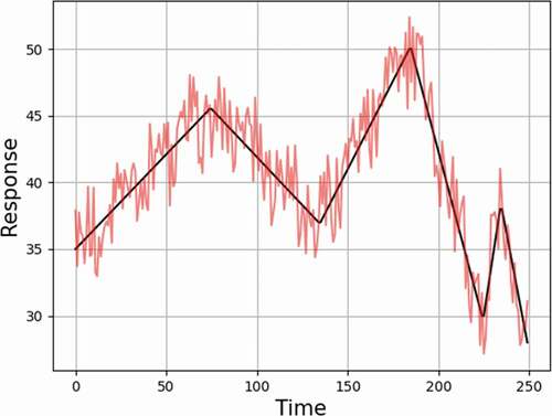
The basic idea of triangle attack is that given a sequence of measurements, i.e., signal values of a process variable containing noise, a series of line segments is calculated to adjust the trend of the process variable variations with artifact noise added to emulate the noise in the raw data before they are falsified. Calculation of these line segments does not require knowledge about the dynamical model governing the system behavior as it employs simple rules to find the best linear trends and then superimposes noise that is consistent with the noise in the raw data as illustrated in Fig. 7. The red noisy data set represents the raw measurements, and the black line segments represent the calculated trends. The falsified data represent the sum of the linear trends, to be selected by the attacker to change the system state, and artifact noise designed to evade replay attack detection. The detailed calculational procedures of the triangle attack may be found in Ref. 7.

Fig. 7. Line segment fit of triangle attack.⁷

As mentioned earlier, a key contribution of this paper is the design of a denoising algorithm to ensure that subtle variations can be distinguished from the noise. To measure the impact of the noise, two signal-to-noise (S/N) ratio types of metrics are employed, defined as the ratio of the noisy signal to the noise within the attack region, mathematically expressed as S_noisy/N. Another metric is employed as a measure of the meaningful signal, defined as the ratio of the noise-free signal to the noise within the attack window, mathematically expressed as S_clean/N, where S_noisy, S_clean, and N are defined in Eq. (20)(20) $\begin{array}{rl}& S_{noisy}=\sqrt{\frac{\sum _{l=1}^{w_a}{(y_l^g-y_l^a)}^2}{w_a}}\mathrm{o}\mathrm{v}\mathrm{e}\mathrm{r}\mathrm{t}\mathrm{h}\mathrm{e}\mathrm{a}\mathrm{t}\mathrm{t}\mathrm{a}\mathrm{c}\mathrm{k}\mathrm{w}\mathrm{i}\mathrm{n}\mathrm{d}\mathrm{o}\mathrm{w},\\ & S_{clean}=\sqrt{\frac{\sum _{l=1}^{w_a}{(y_l^{g_0}-y_l^{a_0})}^2}{w_a}}\mathrm{o}\mathrm{v}\mathrm{e}\mathrm{r}\mathrm{t}\mathrm{h}\mathrm{e}\mathrm{a}\mathrm{t}\mathrm{t}\mathrm{a}\mathrm{c}\mathrm{k}\mathrm{w}\mathrm{i}\mathrm{n}\mathrm{d}\mathrm{o}\mathrm{w},\\ & \mathrm{a}\mathrm{n}\mathrm{d}\\ & N=\sqrt{\frac{\sum _{l=1}^{w_a}{(y_l^{g_0}-y_l^g)}^2}{w_a}}\mathrm{o}\mathrm{v}\mathrm{e}\mathrm{r}\mathrm{t}\mathrm{h}\mathrm{e}\mathrm{a}\mathrm{t}\mathrm{t}\mathrm{a}\mathrm{c}\mathrm{k}\mathrm{w}\mathrm{i}\mathrm{n}\mathrm{d}\mathrm{o}\mathrm{w}.\end{array}$(20) :

(20) $\begin{array}{rl}& S_{noisy}=\sqrt{\frac{\sum _{l=1}^{w_a}{(y_l^g-y_l^a)}^2}{w_a}}\mathrm{o}\mathrm{v}\mathrm{e}\mathrm{r}\mathrm{t}\mathrm{h}\mathrm{e}\mathrm{a}\mathrm{t}\mathrm{t}\mathrm{a}\mathrm{c}\mathrm{k}\mathrm{w}\mathrm{i}\mathrm{n}\mathrm{d}\mathrm{o}\mathrm{w},\\ & S_{clean}=\sqrt{\frac{\sum _{l=1}^{w_a}{(y_l^{g_0}-y_l^{a_0})}^2}{w_a}}\mathrm{o}\mathrm{v}\mathrm{e}\mathrm{r}\mathrm{t}\mathrm{h}\mathrm{e}\mathrm{a}\mathrm{t}\mathrm{t}\mathrm{a}\mathrm{c}\mathrm{k}\mathrm{w}\mathrm{i}\mathrm{n}\mathrm{d}\mathrm{o}\mathrm{w},\\ & \mathrm{a}\mathrm{n}\mathrm{d}\\ & N=\sqrt{\frac{\sum _{l=1}^{w_a}{(y_l^{g_0}-y_l^g)}^2}{w_a}}\mathrm{o}\mathrm{v}\mathrm{e}\mathrm{r}\mathrm{t}\mathrm{h}\mathrm{e}\mathrm{a}\mathrm{t}\mathrm{t}\mathrm{a}\mathrm{c}\mathrm{k}\mathrm{w}\mathrm{i}\mathrm{n}\mathrm{d}\mathrm{o}\mathrm{w}.\end{array}$(20)

In our context, both signals refer to the difference between the genuine and the falsified data, where the subscripts g and a refer to genuine signals and attack signals, respectively; the subscript l refers to the temporal index of the profiles; the attack window length is denoted as w_a. The noise is defined as the discrepancy between the raw sensor readings $y_l^g$and the simulated signals $y_l^{g_0}$, where the subscript 0 represents noise-free profiles. To construct the attack, the meaningful signal, i.e., S_clean, should match the noise level or even be smaller.

IV.B. Univariate FDI Detection with Multilevel Denoising Approach

This section applies the OT defense to a single monitored process variable, using a two-level denoising methodology. For the first level, the first two column vectors in U₁ in Eq. (16)(16) ${\stackrel{\mathbf{ˆ}}{\mathbf{H}}}^i={\mathbf{U}}_1{\mathbf{U}}_2{\mathbf{U}}_3\cdots {\mathbf{U}}_m{\mathbf{U}}_m^T\cdots {\mathbf{U}}_3^T{\mathbf{U}}_2^T{\mathbf{U}}_1^T{\mathbf{H}}^i,$(16) are used per Eq. (7(7) ${\mathbf{H}}^{\mathrm{R}\mathrm{e}\mathrm{f}}\mathbf{=}\mathbf{U}\mathbf{S}{\mathbf{V}}^T\approx \sum _{k=1}^r{s}_k{\mathbf{u}}_k{\mathbf{v}}_k^T,$(7) ), and for the second level, the first column vector in U₂ is used. The window size for the temporal level w is taken as 20, and the window size for the component level v is 10. The time delay resulting from denoising is 29 time steps based on Eq. (17)(17) $T=\sum _{l=1}^m{w}_l-1,$(17) .

The results are shown in the subplots in Figs. 8, 9, and 10. In Figs. 8a, 9a, and 10a, the noisy genuine and attack temporal profiles of the monitored process variable, the temperature at the primary side of the SG, are shown as green and red dashed lines separately, and the non-noisy genuine and attack temporal evolutions are plotted as blue and orange solid lines, respectively. The added noise profile follows a normal distribution with the mean value as 0 and the standard deviation as 0.2%. The noisy profile is calculated via Eq. (21)(21) $y_i=(1+n_i)\cdot y_i^0,$(21) :

(21) $y_i=(1+n_i)\cdot y_i^0,$(21)

Fig. 8. Univariate FDI detection with multilevel denoising (region 1).

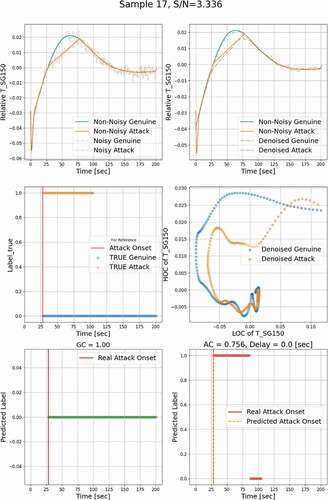
Fig. 9. Univariate FDI detection with multilevel denoising (region 2).

where

$y_i$ =	=	noisy sensor readings
$n_i$ =	=	added noise
$y_i^0$ =	=	noise-free/simulated variable
$i$ =	=	index of the time step.

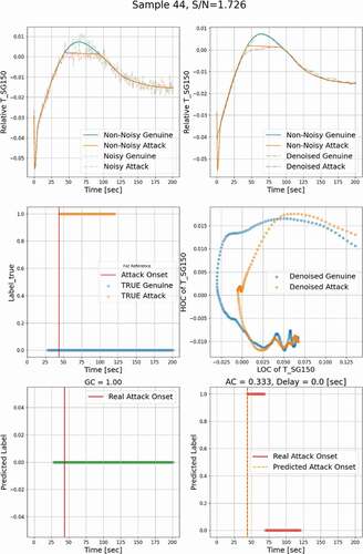
Figures 8b, 9b, and 10b show the denoised temporal evolution of the monitored process variable. The noisy profiles are also represented here for a complete demonstration of results. Figures 8d, 9d, and 10d contain the relationship between the LOC and the HOC features extracted from genuine and attack signals. Here, the genuine datasets and the other datasets containing falsified data are labeled ‘0’ and ‘1,’ respectively. In Figs. 8c, 9c, and 10c, the blue horizontal dots show the true labels of genuine input datasets as a function of time, and the orange dots show the labels of attack datasets. Ideally, for a given genuine profile, the OT defense should issue a ‘0’ label for all the time steps, i.e., GC = 1.0, and for an attack profile, it should issue a ‘1’ label over the attack window, i.e., AC = 1.0, whose onset is marked by a vertical red solid line. Figures 8e, 9e, and 10e show the prediction of the OT defense when a genuine profile is applied; i.e., all predicted labels are ‘0’ as would be expected. Figures 8f, 9f, and 10f show the results when the OT defense is presented with an attack profile. Results shows that a label ‘1’ is declared 0.0 to 50.0 s after the onset of the attack, and the cases with delay not less than 50 s are considered as undetected.

With the premise stated in Sec. II.E, here, the alarming time limit is selected as 5 s, and the difference limit expressed in Eq. (19)(19) $d_l=\sqrt{\frac{\sum _{l=1}^{w_a}{(y_l^g-y_l^a)}^2}{w_a}},$(19) is chosen as 0.35%. In other words, when the noisy discrepancy between the genuine and the attack data within the attack window is over 0.35% of the standardized profile, the attack is considered a valid attack; if the predicted alarming time lasts over 5 s, the attack can be considered detected. The detection performance is evaluated by AC, GC, and detection delay, which are shown by the subtitles of Figs. 8e, 9e, and 10e and Figs. 8f, 9f, and 10f. The sample index and the corresponding S/N ratio S_clean/N are represented by the titles in Figs. 8, 9, and 10.

The simulation has been executed 1000 times, all representing a range of operational conditions, achieved by randomly sampling initial and boundary conditions as well as some of the model’s parameters. In total, 750 samples were used to train the classifier, and the remaining 250 samples were used for testing. For each of the training samples, an attack window was randomly placed, and the trend was changed to piecewise linear. Noise was added to both the original values (representing genuine behavior) and the attack values. Based on the position of the attack windows, we selected three different attack regions for demonstration, i.e., regions where the given response is increasing (Fig. 8), decreasing (Fig. 10), and in-between where a peak is expected (Fig. 9). These three regions will be denoted by “increasing,” “decreasing,” and “peak,” respectively.

Fig. 10. Univariate FDI detection with multilevel denoising (region 3).

Figure 8 shows an example of FDI detection results using the developed multilevel denoising method, in which the attack is injected in the increasing region. Analysis of the relationship between the HOC and the LOC in Fig. 8b reveals that a small difference in the temporal evolution of a response could lead to a significant difference in the HOC-LOC pattern, based on which classifier can be reliably trained. The classifier predicted labels for genuine data are shown in Fig. 8e, all as ‘0,’ indicating that the classifier will not misclassify the genuine data as attacked data and issue a false alarm. In Fig. 8f, the predicted labels for attack data represent ‘1’ without a time delay. Figure 8e shows that the classifier is triggered at 75.6% of the time when the monitoring and attack window overlap, i.e., AC = 0.756. Based on the 5-s detection criterion, this attack is hence detectable. Similar results for the peak and decreasing regions are shown in Figs. 9 and 10, respectively.

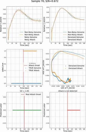
To have an overall assessment of the detection results for all 250 analyzed test cases, the relationship between the clean S/N ratio, S_clean/N, and the detection delay time is plotted in Fig. 11. The results show a trend that for a higher S/N ratio, the detection delay time will be shorter, and vice versa. The detectable limit of the S_clean/N ratio is 0.933, shown as a red horizontal dashed line, demonstrating that when the S_clean/N ratio is above this limit, the attack can always be detected. For the cases that are not detected, their meaningful clean signal is very small because the attack and the genuine track almost match each other; an example is shown in Fig. 12.

Fig. 11. Detection delay time versus S/N ratio with univariate monitoring.

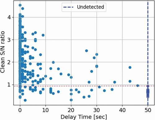
Fig. 12. Example of undetected attack.

IV.C. Multivariate FDI Detection with Multilevel Denoising Approach

Section IV.B focused on analyzing behavior using the LOC and the HOC associated with a single response; i.e., no correlation between responses is employed. In this section, the LOCs and the HOCs obtained from different responses are employed to design the classifier. Intuitively, this is sought to improve the performance of the classifier. An important step here is to devise a procedure by which the best LOCs and HOCs from a group of responses are selected to train the classifier. By way of an example, consider two responses, T_SG150 and T_SG210, and consider a single LOC and a single HOC associated with each one of them. A brute force approach could be used to incorporate all HOCs and LOCs from multiple responses; however, this is expected to overwhelm the training. Instead, we employ a simple criterion, that is, to select the pair of features with the highest mutual information. This can be calculated using kernel density estimation of the joint probability distribution. An example is shown in Fig. 13, where Fig.13c shows the best pair of features. Here, this can be eyeballed by identifying the two features showing the most correlation, i.e., least uncertainty. A more sophisticated selection criterion based on the fusion of multiple features from multiple responses will be sought in our future work.

Fig. 13. Component correlation of different process variables.

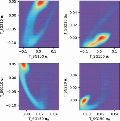
Figures 13a through 13d plot the components from two process variables among all samples; the red areas indicate where the component data accumulate, and the purple areas indicate less data accumulation. T_SG150 represents the temperature at the primary side of the SG, and T_SG210 represents the temperature at the secondary side of the SG. The LOC and the HOC from each process variable are denoted as ${\alpha }_L\mathrm{a}\mathrm{n}\mathrm{d}{\alpha }_H,$ respectively. From Fig. 13, one can see there is a trend in every subplot. In other words, the components recorded by the x-axis are dependent on the ones for the y-axis. This section focuses on the question of whether this dependence can be leveraged to find subtle inconsistency within the data. To validate this point, the same attack window in Sec. IV.B is injected into the temporal signal profile of T_SG150, but the feature construction involves correlated LOCs and HOCs from different process variables.

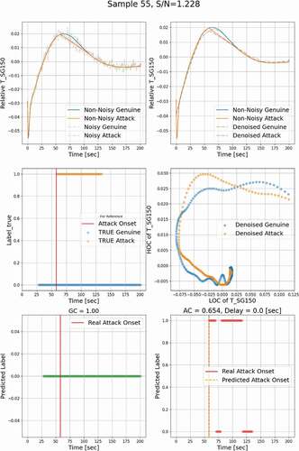
The next set of figures, Figs. 14, 15, and 16, repeats the detection results but now uses the LOCs and HOCs from two different responses. It is assumed that the first response T_SG150 is attacked whereas the other response T_SG210 is not attacked. The classifier is trained based on a single LOC of T_SG150 and a single HOC of T_SG210 as plotted in Fig. 14d. Figure 14b shows the noisy, non-noisy, and denoised temporal profiles of T_SG210. The non-noisy temporal evolution of T_SG210 is shown as the orange solid curve, the green dashed line represents the T_SG210 temporal profile with evolution, and the denoised profile is represented as a blue curve. From the results, one can tell that compared to univariate monitoring, the attack data detection coverage increases from AC = 0.756 to AC = 1.0 with two responses used for monitoring. Similar behavior is observed for the peak region, where AC increased from 0.33 to 0.821. For the decreasing region, AC did not change much because the attack has a very similar trend to the genuine profile.

Fig. 14. Multivariate FDI detection with multilevel denoising (region 1).

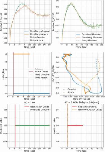
Fig. 15. Multivariate FDI detection with multilevel denoising (region 2).

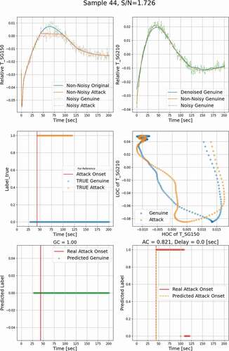
Fig. 16. Multivariate FDI detection with multilevel denoising (region 3).

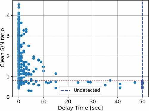
Similar to the results shown earlier, Fig. 17 shows the relationship between the clean S/N ratio and the delayed detection time, but now there are two responses used for monitoring. For multivariate monitoring, the S_clean/N detectable limit is 0.726, shown as the red dashed line, which is lower than the limit of univariate monitoring.

Fig. 17. Detection delay time versus S/N ratio with multivariate monitoring.

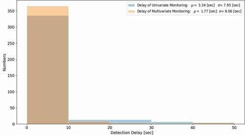
Figure 18 shows a histogram of the detection delay of the monitoring results with a single response and two responses, which indicates that multivariate monitoring reduces the detection delay by almost 50%. The mean value of the detection delay is 1.77 s for multivariate monitoring and is 3.34 s for univariate monitoring; the standard deviation of the delay time is smaller for multivariate monitoring.

Fig. 18. Histogram comparison of detection delay.

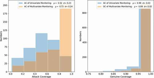
Scatter plots in Fig. 19 represent the relationship between the two S/N ratios; different colors indicate the different time periods of the detection delay. Most attacks can be detected within 10 s, shown as yellow dots, and there are fewer long-time detection delay cases in multivariate monitoring. And, for both monitoring approaches, the cases with a longer detection time occur at the low S/N region. Finally, Fig. 20 shows the AC values using both univariate and multivariate monitoring. The results indicate a clear shift of the AC values when additional responses are used for monitoring.

Fig. 19. Relationship between clean and total S/N ratio with detection delay.

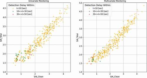
Fig. 20. Histogram of AC and GC for both monitoring methods.

Before concluding, it is important to remark that the computational cost for the proposed detection algorithm may be split into two components: an off-line component and an online component. The off-line component comprises the computational cost to design the HOCs and the LOCs, which can be done during a training phase. Further, because all the attack scenarios are based on the idea of triangle attacks, the training of the classifier can also be completed off-line. This represents the key cost of the overall algorithm as the online component involves only the projection of the windowed time series over the HOC/LOC components (which are simple inner product operations) and the execution of the already-trained classifier; both are essentially instantaneous.

V. CONCLUSIONS

Industrial control systems have been upgraded with digital instrumentations for efficient control, operational convenience, and expeditious data traffic. Despite the numerous benefits of digitization, one must address the threats posed by potential adversaries looking for vulnerabilities. Previous studies demonstrate two key results: (1) the attacker can learn the system behavior to a reasonable approximation solely with historical data and (2) equipped with an approximate physics model and historical data, the attacker can reverse-engineer the missing details of the model, e.g., model parameters, and make accurate predictions of the system behavior. With learned system behavior, attackers can launch stealthy attacks to circumvent the detection by conventional monitoring techniques.

This paper proposes a real-time monitoring method for FDI attack detection that is supported by a multilevel denoising approach to allow the detection of subtle variation under the presence of process noise. The idea for detection is to rely both on dominant features, referred to as LOCs, and on less dominant features, referred to as HOCs, to derive features that can identify FDI attacks. The results indicate that the patterns established by the LOCs and the HOCs could be very effective in detecting subtle variations, expected to be the mode of attack during an initial lie-in-wait period, used to test the attacker’s ability to bypass detection.

The results also indicate that attacks comparable to the noise level can be detected, with the detection ability improved with additional responses used for monitoring. This is especially important for replay attack, which relies on using older genuine data to spoof future sensor readings.

Several outstanding developments need to be further addressed in support of this work. For example, when employing multiple sensors for monitoring, a general methodology is required to downselect the features from the available sensors. In this work, a simple criterion based on the use of mutual information is used. Also, a more detailed analysis of the binary classification results is needed to design a better detection criterion by analyzing the relationship of the points to trigger the alarm to the classifier’s decision boundary.

Acknowledgments

This work was supported by the Idaho National Laboratory (Laboratory Directed Research and Development) and the U.S. Department of Energy (DE-NE0008705).

References

- R. LANGNER, “Stuxnet: Dissecting a Cyberwarfare Weapon,” IEEE Secur. Priv., 9, 3, 49 (2011); https://doi.org/https://doi.org/10.1109/MSP.2011.67.
- “Monju Power Plant Facility PC Infected with Virus,” Japan Today (2014); https://japantoday.com/category/national/monju-power-plant-facility-pc-infected-with-virus (current as of Apr. 19, 2021).
- C. STEITZ and E. AUCHARD, “German Nuclear Plant Infected with Computer Viruses, Operator Says,” Reuters (2016); https://www.reuters.com/article/us-nuclearpower-cyber-germany/german-nuclear-plant-infected-with-computer-viruses-operator-says-idUSKCN0XN2OS (current as of Apr. 19, 2021).
- “2017 Cyberattacks on Ukraine,” Wikipedia; https://en.wikipedia.org/wiki/2017_cyberattacks_on_Ukraine (current as of Apr. 19, 2021).
- “ North Korean Hacks on India Seek Data, Not Disruption,” in “Expert Briefings,” Oxford Analytica (2019); https://doi.org/https://doi.org/10.1108/OXAN-ES247614.
- J. PEISER, “A Hacker Broke into a Florida Town’s Water Supply and Tried to Poison It with Lye, Police Said,” The Washington Post (2021); https://www.washingtonpost.com/nation/2021/02/09/oldsmar-water-supply-hack-florida/ (current as of Apr. 19, 2021).
- J. LARSEN, “Miniaturization” (2014); https://www.blackhat.com/docs/us-14/materials/us-14-Larsen-Miniturization-WP.pdf.
- Y. LI and H. S. ABDEL-KHALIK, “Data Trustworthiness Signatures for Nuclear Reactor Dynamics Simulation,” Prog. Nucl. Energy, 133, 103612 (2021); https://doi.org/https://doi.org/10.1016/j.pnucene.2020.103612.
- A. SUNDARAM, H. S. ABDEL-KHALIK, and O. ASHY, “A Data Analytical Approach for Assessing the Efficacy of Operational Technology Active Defenses Against Insider Threats,” Prog. Nucl. Energy, 124, 103339 (2020); https://doi.org/https://doi.org/10.1016/j.pnucene.2020.103339.
- Y. ZHAO and C. SMIDTS, “A Control-Theoretic Approach to Detecting and Distinguishing Replay Attacks from Other Anomalies in Nuclear Power Plants,” Prog. Nucl. Energy, 123, 103315 (2020); https://doi.org/https://doi.org/10.1016/j.pnucene.2020.103315.
- A. SUNDARAM, H. S. ABDEL-KHALIK, and O. ASHY, “Exploratory Study into the Effectiveness of Active Monitoring Techniques,” Trans. Am. Nucl. Soc., 121, 198 (2019); https://doi.org/https://doi.org/10.13182/T31258.
- A. SUNDARAM and H. ABDEL-KHALIK, “Covert Cognizance: A Novel Predictive Modeling Paradigm,” Nucl. Technol., 207, 1163 (2021); https://doi.org/https://doi.org/10.1080/00295450.2020.1812349.
- S. L. EGGERS, “Adapting Anomaly Detection Techniques for Online Intrusion Detection in Nuclear Facilities,” PhD Dissertation, University of Florida (2018); https://ufdcimages.uflib.ufl.edu/UF/E0/05/21/34/00001/EGGERS_S.pdf (current as of Apr. 19, 2021).
- F. ZHANG and J. B. COBLE, “Robust Localized Cyber-Attack Detection for Key Equipment in Nuclear Power Plants,” Prog. Nucl. Energy, 128, 103446 (2020); https://doi.org/https://doi.org/10.1016/j.pnucene.2020.103446.
- W. WANG, F. DI MAIO, and E. ZIO, “A Non-Parametric Cumulative Sum Approach for Online Diagnostics of Cyber Attacks to Nuclear Power Plants,” Resilience of Cyber-Physical Systems, Springer (2019).
- H. L. GAWAND, A. K. BHATTACHARJEE, and K. ROY, “Securing a Cyber Physical System in Nuclear Power Plants Using Least Square Approximation and Computational Geometric Approach,” Nucl. Eng. Technol., 49, 3, 484 (2017); https://doi.org/https://doi.org/10.1016/j.net.2016.10.009.
- Y. ZHAO et al., “Finite-Horizon Semi-Markov Game for Time-Sensitive Attack Response and Probabilistic Risk Assessment in Nuclear Power Plants,” Reliab. Eng. Syst. Saf., 201, 106878 (2020); https://doi.org/https://doi.org/10.1016/j.ress.2020.106878.
- P. K. VADDI et al., “Dynamic Bayesian Networks Based Abnormal Event Classifier for Nuclear Power Plants in Case of Cyber Security Threats,” Prog. Nucl. Energy, 128, 103479 (2020); https://doi.org/https://doi.org/10.1016/j.pnucene.2020.103479.
- J. LI and X. HUANG, “Cyber Attack Detection of I&C Systems in NPPS Based on Physical Process Data,” Proc. 24th Int. Conf. Nuclear Engineering (ICONE), Charlotte, North Carolina, June 26–30, 2016, Vol. 2, ASME (2016); https://doi.org/https://doi.org/10.1115/ICONE24-60773.
- Y. LIU, P. NING, and M. K. REITER, “False Data Injection Attacks Against State Estimation in Electric Power Grids,” ACM Trans. Information and Systems Security, 14, 1, 1 (2011); https://doi.org/https://doi.org/10.1145/1952982.1952995.
- Y. LI et al., “ROM-Based Surrogate Systems Modeling of EBR-II,” Nucl. Sci. Eng., 195, 520 (2021); https://doi.org/https://doi.org/10.1080/00295639.2020.1840238.
- Y. LI and H. ABDEL-KHALIK, “ROM-Based Subset Selection Algorithm for Efficient Surrogate Modeling,” Trans. Am. Nucl. Soc., 115, 1740 (2016).
- D. HUANG et al., “Dimensionality Reducibility for Multi-Physics Reduced Order Modeling,” Ann. Nucl. Energy, 110, 526 (2017); https://doi.org/https://doi.org/10.1016/j.anucene.2017.06.045.
- C. CORTES and V. VAPNIK, “A Fast SVD for Multilevel Block Hankel Matrices with Minimal Memory Storage,” Numer. Algorithms, 69, 875 (2015); https://doi.org/https://doi.org/10.1007/s11075-014-9930-0.
- A. SUNDARAM, Y. LI, and H. S. ABDEL-KHALIK, “A Multi-Level Feature Extraction and Denoising Approach to Detect Subtle Variations in Industrial Control Systems,” Proc. Int. Conf. Mathematics and Computational Methods Applied to Nuclear Science and Engineering (M&C 2021), Virtual Conference, October 3–7, 2021, American Nuclear Society (2021).
- “RELAP5/MOD3.3 Code Manual Volume III: Developmental Assessment,” Vol. III, Idaho National Laboratory (2006).
- M. P. PETERSON and C. E. PAULSEN, “An Implicit Steady-State Initialization Package for the RELAP5 Computer Code,” NUREG/CR-6325, U.S. Nuclear Regulatory Commission (1995).