Frequency Transform Method for Transient Analysis of Nuclear Reactors in Monte Carlo

Abstract

The Frequency Transform method is used for the first time to efficiently model a multiple-second transient problem with Monte Carlo (MC). This is achieved by coupling MC with a time-dependent coarse mesh finite difference (TD-CMFD) diffusion solver. TD-CMFD presents a large advantage over commonly used point kinetics equations since it preserves spatial resolution during the transient and provides equivalence with the high-order method through nonlinear diffusion coefficients. As TD-CMFD computes time-dependent and spatially dependent neutronics information, it also computes frequencies that describe the rate of change of neutron and delayed precursor concentrations. These frequencies are used in MC shape function calculations as an approximation for the time derivatives. As the simulation proceeds, MC calculations update the multigroup cross sections, currents, and diffusion coefficients that are needed in TD-CMFD, and in turn, TD-CMFD updates the frequencies. Our results show the success of the Frequency Transform method in prescribed transient problems on the C5G7 geometry and on a fuel pin geometry. The Frequency Transform method showed significant improvement compared to the Adiabatic approximation, which does not use any frequency information in the MC calculation. The improvements in spatial resolution are shown to be a direct result of frequencies.

Keywords:

• Monte Carlo
• transient
• frequency transform
• coarse mesh finite difference

View correction statement:

Correction

I. INTRODUCTION

High-fidelity simulation of nuclear reactors plays an important role in ensuring the safe and profitable generation of electricity at existing power plants as well as in the deployment of advanced reactor designs. Monte Carlo (MC) methods are the preferred high-fidelity tool for neutronics calculations, but time-dependent analysis by MC is still considered prohibitively costly in large reactors for long transients (on the order of 10 s). Today, standard industrial codes like SIMULATE3-K (Ref. 1) couple their kinetics methods with diffusion solvers [nodal methods or coarse mesh finite difference (CMFD)]. The use of MC in transients is the next breakthrough for high-fidelity modeling, but its efficient implementation is a hurdle. The standard technique for expanding such expensive calculations is to carry out the expensive calculation (in this case, MC) as a high-order method over long time steps and using a low-order calculation over short time steps, referred to as a high-order/low-order (HOLO) scheme. Figure 1 illustrates this time-stepping scheme. The expensive, high-order MC calculations occur at the blue markers while the low-order neutronics approximation occurs at the green markers.

Fig. 1. Time-stepping scheme for time-dependent MC problems.

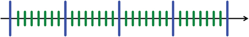
For this time-stepping scheme to work, it is assumed that the flux shape of the problem is slowly moving, so it can be updated at the infrequent blue markers, while the amplitude is quickly moving, so it needs to be updated often on the green markers. Decomposing flux into shape and amplitude components is shown in Eq. (1)(1) $\mathrm{\Psi }(r,E,\mathrm{\Omega },t)=\psi (r,E,\mathrm{\Omega },t)\varphi (r,E,\mathrm{\Omega },t),$(1) :

(1) $\mathrm{\Psi }(r,E,\mathrm{\Omega },t)=\psi (r,E,\mathrm{\Omega },t)\varphi (r,E,\mathrm{\Omega },t),$(1)

where

$\mathrm{\Psi }$	=	= full angular flux
$\psi$	=	= shape function of the flux
$\varphi$	=	= amplitude function of the flux.

Historically, the point kinetics equations have been widely used as the lower-order method in time-dependent calculations. Point kinetics use the initial shape function of the flux and assume the amplitude is only a time-dependent scalar, resulting in poor spatial resolution. In this paper, the Frequency Transform method will be introduced to preserve the spatial dependence of the flux amplitude by using a time-dependent coarse mesh finite difference (TD-CMFD) solver instead of point kinetics. This work solves time-dependent diffusion where equivalence factors and cross sections are provided from high-fidelity, frequency-transformed MC. This formulation was recently published² and will be further demonstrated in this paper. First, results from Ref. 2 will be reproduced to show that our implementation is correct, and further problems will be carried out to demonstrate the impact of frequencies in transient problems and the evolution of multigroup parameters during a HOLO transient.

II. METHODS

II.A. Frequency Transform Method

Coupling MC and CMFD is ideal for transients on the order of a few seconds since no nuclide transmutation or buildup is included. The two solvers exchange information based on the frequency transform formulation of the neutron transport equation. The Frequency Transform method approximates the derivative terms of the transport equation with exponential frequencies as shown in the following derivation. The Frequency Transform method approximates the amplitude as an exponential:

(2) $\mathrm{\Psi }(r,E,\mathrm{\Omega },t)=\psi (r,E,\mathrm{\Omega },t)e^{{\omega }^P(r,E,\mathrm{\Omega },t)\cdot t}.$(2)

In the time-differencing scheme used here, the frequencies of the prompt neutron population ${\omega }^P(r,E,\mathrm{\Omega },t)$ are computed as needed when the simulation returns to the MC calculation. As such, the frequencies are considered instantaneous, and therefore, their time dependence can be neglected (not because they are constant but because they are instantaneous). With this in mind, we differentiate with respect to time:

(3) $\frac{\mathrm{\partial }\mathrm{\Psi }}{\mathrm{\partial }t}=\frac{\mathrm{\partial }\psi }{\mathrm{\partial }t}{e}^{{\omega }^P\cdot t}+\psi {\omega }^P{e}^{{\omega }^P\cdot t}.$(3)

If the frequencies are properly chosen, the shape function is slowly varying relative to the amplitude function. In fact, since the amplitude is computed in both time and space by the TD-CMFD solver and since the frequencies are calculated using the last inner time step, these are considered quite accurate. Therefore, we approximate the derivative of the shape function to be zero (Refs. 3 and 4). If the Frequency Transform method were applied to the TD-CMFD solver, the time derivative of the shape function could be expressed in a time-differencing scheme. However, in this work, the diffusion solver is so efficient relative to the MC solver that diffusion is performed using the full scalar flux in an implicit scheme. Monte Carlo, however, benefits greatly from the approximation. This leads to

(4) $\frac{\mathrm{\partial }\mathrm{\Psi }}{\mathrm{\partial }t}=\psi {\omega }^P{e}^{{\omega }^P\cdot t}$(4)

(5) $\frac{1}{v}\frac{\mathrm{\partial }\mathrm{\Psi }}{\mathrm{\partial }t}=\frac{1}{v}{\omega }^P\mathrm{\Psi }.$(5)

Likewise, the precursor concentrations can be frequency transformed to yield

(6) $\frac{\mathrm{\partial }C}{\mathrm{\partial }t}={\omega }^{D}C.$(6)

So, ${\omega }^{P,g}$ is the prompt neutron frequency for each energy group $g$, and ${\omega }^{D,b}$ is the delayed neutron frequency for each precursor group $b$. Both can be phase-space dependent and are calculated “instantaneously” using the most up-to-date information from the inner time steps. When used in the time-dependent neutron transport equation in place of time derivatives, these frequency transforms eliminate the need to evaluate any time derivative terms altogether. This Frequency Transform method is also sometimes referred to as the exponential transform or $\omega$-mode.^3,4 In a slightly different form, exponential frequencies have also been used as a stiffness confinement method similar to treating prompt and delayed neutrons separately.^5,6

II.B. Time-Dependent Coarse Mesh Finite Difference

The value of the frequencies is determined for each cell, energy group, and precursor group during the TD-CMFD calculations. By definition, CMFD is a diffusion solver with an additional nonlinear diffusion coefficient term. This term is a correction term that is required for consistency between the high- and low-order methods. In this case, it is used to maintain local consistency between MC and diffusion. This has been demonstrated very successfully when CMFD is coupled to method of characteristics solvers.^7,8 TD-CMFD receives information from MC such as multigroup cross sections, currents, and diffusion coefficients. With that information, the TD-CMFD solver can carry out the time-dependent transient for a number of time steps. Since the MC calculations are the most expensive part of the simulation, the TD-CMFD solver should be carried out for as long as possible, keeping the total number of MC calculations small. The calculation returns to MC whenever the change in the frequency becomes large or after a fixed number of time steps.

The frequencies at a given time $t_n$ are related to the flux and precursor concentration as follows:

(7) $e^{{\omega }^{P,g}\mathrm{\Delta }{t}_n}{\varphi }_{t_{n-1}}^g={\varphi }_{t_n}^g$(7)

(8) $\Rightarrow {\omega }^{P,g}=\frac{1}{\mathrm{\Delta }{t}_n}\mathrm{l}\mathrm{o}\mathrm{g}\frac{{\varphi }_{t_n}^g}{{\varphi }_{t_{n-1}}^g}$(8)

and

(9) $e^{{\omega }^{D,b}\mathrm{\Delta }{t}_n}{C}_{t_{n-1}}^b=C_{t_n}^b$(9)

(10) $\Rightarrow {\omega }^{D,b}=\frac{1}{\mathrm{\Delta }{t}_n}\mathrm{l}\mathrm{o}\mathrm{g}\frac{C_{t_n}^b}{C_{t_{n-1}}^b}.$(10)

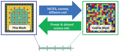
At the end of the TD-CMFD time, the instantaneous frequencies are computed and passed to MC. They represent the current state of the prompt neutron and delayed precursor populations. These frequencies serve as the approximation for the derivative term in the transport equation and therefore become inputs to MC. During the MC calculation, multigroup cross sections, cell currents, and diffusion coefficients are tallied and passed to the TD-CMFD solver. In summary, Fig. 2 shows how the two solvers communicate with each other.

Fig. 2. Communication diagram between the high-order MC solver and the low-order TD-CMFD solver.

II.C. Comparison to Other Methods

Most transient methods require a HOLO approach to be computationally tractable, and the method presented in this paper is often compared to existing methods that share similarities. To put the Frequency Transform method into perspective, we include a summary of other existing methods and how they differ from each other. Those differences will mostly revolve around the approximation made to the time derivatives in the high-order method. A detailed quantitative comparison of these methods on a common benchmark can be found in Ref. 9.

II.C.1. Adiabatic Method

In the Adiabatic approximation, the transient is assumed to be happening slowly enough that the system can be approximated by its instantaneous eigenstate. As such, the time derivatives for flux and precursor concentrations are zeroed-out in the high-order method; see Eqs. (11)(11) $\frac{\mathrm{\partial }{\mathrm{\Psi }}^g}{\mathrm{\partial }t}=0$(11) and (12(12) $\frac{\mathrm{\partial }{C}^b}{\mathrm{\partial }t}=0.$(12) ):

(11) $\frac{\mathrm{\partial }{\mathrm{\Psi }}^g}{\mathrm{\partial }t}=0$(11)

and

(12) $\frac{\mathrm{\partial }{C}^b}{\mathrm{\partial }t}=0.$(12)

This amounts to solving only a steady-state system at the high-order calculation.

II.C.2. Omega Method

In the Omega-mode, as discussed at length in this paper, the high-order calculation is time dependent, with time dependence terms given from the lower-order method in the form of frequencies; see Eqs. (13)(13) ${\mathrm{\Psi }}^g={\psi }^g{e}^{{\omega }^{P,g}t}$(13) and (14(14) $\frac{\mathrm{\partial }{\mathrm{\Psi }}^g}{\mathrm{\partial }t}={\omega }^{P,g}{\mathrm{\Psi }}^g$(14) ):

(13) ${\mathrm{\Psi }}^g={\psi }^g{e}^{{\omega }^{P,g}t}$(13)

and

(14) $\frac{\mathrm{\partial }{\mathrm{\Psi }}^g}{\mathrm{\partial }t}={\omega }^{P,g}{\mathrm{\Psi }}^g$(14)

and

(15) $\frac{\mathrm{\partial }{C}^b}{\mathrm{\partial }t}={\omega }^{D,b}{C}^b.$(15)

If all the frequencies are set to 0, the Omega-mode collapses back to the Adiabatic approximation.

II.C.3. Alpha-Eigenvalue Method

The Alpha-Eigenvalue method is of a slightly different nature than the Adiabatic and Omega methods. In the Alpha-Eigenvalue method, the time derivative of the flux is approximated by a variable alpha. The time derivative of the precursor concentrations is either zeroed-out or also proportional to alpha. See Eqs. (16)(16) $\frac{\mathrm{\partial }{\mathrm{\Psi }}^g}{\mathrm{\partial }t}=\alpha {\mathrm{\Psi }}^g,$(16) , (17(17) $\frac{\mathrm{\partial }{C}^b}{\mathrm{\partial }t}=0,$(17) ), and (18(18) $\frac{\mathrm{\partial }{C}^b}{\mathrm{\partial }t}=\alpha C^b.$(18) ):

(16) $\frac{\mathrm{\partial }{\mathrm{\Psi }}^g}{\mathrm{\partial }t}=\alpha {\mathrm{\Psi }}^g,$(16)

(17) $\frac{\mathrm{\partial }{C}^b}{\mathrm{\partial }t}=0,$(17)

or

(18) $\frac{\mathrm{\partial }{C}^b}{\mathrm{\partial }t}=\alpha C^b.$(18)

Then, an eigenvalue calculation is performed to calculate a single value of alpha that equilibrates the system and acts as the time rate of change. There have been improvements suggested for the Alpha-Eigenvalue method whereby low-order equations provide information about the moments of the angular flux to the high-order solution.^10–12 The technique of sending information from the low-order to the high-order solution is not commonly found in the literature and resembles what is described in this paper. Nonetheless, because of the small or absent amount of information included about delayed neutrons, the Alpha-Eigenvalue method is best suited for supercritical systems. There is also a limitation by only having a single representation of the time rate of change across all energy groups.

II.C.4. Quasi-Static Methods

The Quasi-Static method is a time differencing of the flux and the precursor concentrations while neglecting the time derivative of the shape function.¹³ The Improved Quasi-Static method goes further by keeping the time derivative of the shape function.¹⁴ The Quasi-Static methods make an implicit calculation of the flux and precursors—see Eqs. (19)(19) $\frac{\mathrm{\partial }{\mathrm{\Psi }}^g}{\mathrm{\partial }t}=\frac{{\mathrm{\Psi }}_{n+1}^g-{\mathrm{\Psi }}_n^g}{\mathrm{\Delta }t}$(19) and (20(20) $\frac{\mathrm{\partial }{C}^b}{\mathrm{\partial }t}=\frac{C_{n+1}^b-C_n^b}{\mathrm{\Delta }t}.$(20) )—on a coarse timescale and allow the low-order scheme to fill in the gaps:

(19) $\frac{\mathrm{\partial }{\mathrm{\Psi }}^g}{\mathrm{\partial }t}=\frac{{\mathrm{\Psi }}_{n+1}^g-{\mathrm{\Psi }}_n^g}{\mathrm{\Delta }t}$(19)

and

(20) $\frac{\mathrm{\partial }{C}^b}{\mathrm{\partial }t}=\frac{C_{n+1}^b-C_n^b}{\mathrm{\Delta }t}.$(20)

This makes the method very flexible in accuracy since it can be easily improved by using higher-order time differencing, smaller time steps, and a more robust low-order method. The Improved Quasi-Static method is generally considered among the best representations for transient analysis. However, by definition, it requires time differencing and a fixed source, which are difficult options to implement efficiently in MC, but this has been done in combination with the Dynamic Monte Carlo method.^15,16

II.C.5. Frequency Transform Method

The Frequency Transform method is very similar to the Improved Quasi-Static method with the addition that the time-differenced terms are frequency-transformed; see Eqs. (21)(21) ${\mathrm{\Psi }}^g={\psi }^g{e}^{{\omega }^{P,g}t},$(21) , (22(22) $\frac{\mathrm{\partial }{\mathrm{\Psi }}^g}{\mathrm{\partial }t}=\frac{{\mathrm{\Psi }}_{n+1}^g-{\mathrm{\Psi }}_n^g}{\mathrm{\Delta }t},$(22) ), and (23(23) $\frac{\mathrm{\partial }{C}^b}{\mathrm{\partial }t}=\frac{C_{n+1}^b-C_n^b}{\mathrm{\Delta }t}.$(23) ):

(21) ${\mathrm{\Psi }}^g={\psi }^g{e}^{{\omega }^{P,g}t},$(21)

(22) $\frac{\mathrm{\partial }{\mathrm{\Psi }}^g}{\mathrm{\partial }t}=\frac{{\mathrm{\Psi }}_{n+1}^g-{\mathrm{\Psi }}_n^g}{\mathrm{\Delta }t},$(22)

and

(23) $\frac{\mathrm{\partial }{C}^b}{\mathrm{\partial }t}=\frac{C_{n+1}^b-C_n^b}{\mathrm{\Delta }t}.$(23)

This is identical to the Omega-mode approximation, which represents the amplitude as an exponential. This increases the accuracy of the time-differencing scheme because information from the low-order method can then be incorporated into the coarse time stepping. Again, the nature of the method, with time differencing and a fixed source, make the Frequency Transform method, as originally presented, to be flawed for implementation in MC.

II.C.6. Summary

The Adiabatic and Omega methods use k-eigenvalue solvers to update the shape of the flux at the outer time steps. The Omega method is, by definition, an improvement on the Adiabatic method by not zeroing out the time derivative terms. Additionally, the Omega method has better spatial distribution because of the spatial dependence of the frequencies. The Alpha-Eigenvalue method is comparable to the Omega method and can be modified to resemble it more by modeling delayed neutrons either with $\alpha$ or with frequencies as described further in Ref. 9. The Quasi-Static and Frequency Transform methods are time-differencing schemes that do not rely on eigenvalue solvers. These most closely resemble an implicit solution to the transport equation but are not as amenable to MC simulation. The two methods perform very similarly, with the Improved Quasi-Static method being a generalization of the Frequency Transform method.

Although many of these methods share similarities, the goal of this summary is to expose their differences. In fact, it may appear confusing that the Omega-mode and the Frequency Transform method are described separately. The important difference between the two is that the Frequency Transform method implies that the high-order method will implement time differencing. With the use of MC as the high-order method, this implication is more flexible, and the differences between the Omega-mode and the Frequency Transform method become more ambiguous. This is why they are sometimes used interchangeably.

II.D. Delayed Neutron Modeling

The Dynamic Monte Carlo method explicitly tracks each fission product that is a delayed neutron precursor and then stochastically samples decay and neutron emission.^17–19 There is such a large variation in the timescales of precursor decay that this method is very computationally costly. Furthermore, at any given time, there are thousands more precursors in a problem than neutrons, making the task of tracking them explicitly quite daunting. Nonetheless, this method is widely used, and many variance reduction techniques accompany this method to make it more practical.²⁰ While costly to implement for large reactors, the Dynamic Monte Carlo method is much more convenient for short transients in small geometries such as weapons calculations.²¹

Alternatively, an indirect method for modeling delayed neutrons has been introduced in Ref. 2 to save a significant amount of computation and memory. The precursors are homogenized over small regions, and their concentrations are propagated in time by integrating the precursor balance equation. This assumes the use of solid fuel so precursors are not migrating during the transient. This technique is particularly well suited for TD-CMFD as the homogenized regions can overlap with the mesh used in diffusion.

III. RESULTS

III.A. Impact of Frequencies on Spatial Resolution

We now present example problems carried out with the Frequency Transform method (Omega-mode). The method has been implemented in OpenMC (Ref. 22). The first problem is on the C5G7 geometry.²³ C5G7 is a widely simulated benchmark due to its heterogeneous geometry and the recent addition of time-dependent test problems. The problem modeled here is a modified version of one of the C5G7 benchmarks. It is a prescribed drop in moderator density in the innermost fuel assembly (as opposed to a uniform drop in the whole geometry) with no intrinsic feedback. The transient is fully prescribed, and there is no thermal-hydraulic solver in the simulation. Figures 3 through 7 reproduce the work in Shaner’s thesis² to demonstrate that our implementation in OpenMC correctly reflects the original formulation. This simulation was computed with 1 million particles per batch, with 100 batches including 40 inactive batches. Outer time steps are 0.5 s, inner steps are 0.01 s, and outer time steps were forced to iterate twice. These time steps could be chosen adaptively based on frequency magnitude or the spatial gradient of frequency distribution.

Fig. 3. The core reactivity of the C5G7 geometry under a prescribed moderator density transient for 2 s.

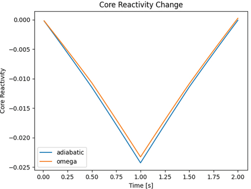
In this 2-s transient, the moderator density drops (only in the top right corner of Fig. 3) to 80% of its value linearly in the first second. Then, it rises back to its original value linearly over the next second. Figure 3 shows the core reactivity change in time, both for the Frequency Transform method and the Adiabatic method. Figure 4 further illustrates the difference between the two methods with the discrepancy in pin powers at 1 s. This difference, which is concentrated in the region of the moderator density change, can be explained by the distribution of the precursor frequencies, shown in Fig. 5. Since the Adiabatic method neglects the frequencies, it fails to capture the extent of the transient. Finally, Figs. 6 and 7 illustrate how the flux and precursor frequencies change in time over the course of the transient.

Fig. 4. Relative difference (%) in pin powers between the Frequency Transform method and Adiabatic approximation at 1 s.

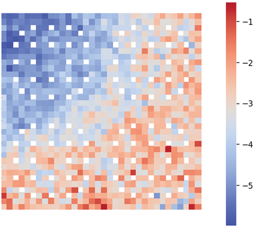
Fig. 5. Spatial distribution of the precursor frequency terms in the C5G7 geometry at 1 s for each of the eight delayed precursor groups (starting at group 1 in the top left-hand corner). Frequencies in units of inverse seconds.

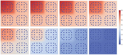
Fig. 6. Evolution of the flux frequency terms in time ($\frac{{\omega }^{P,g}}{v}$).

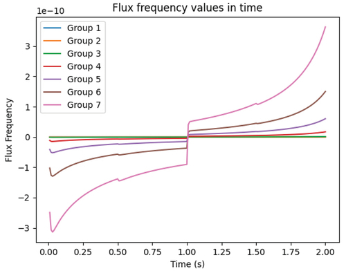
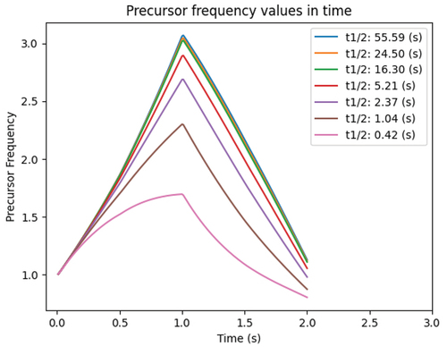
Fig. 7. Evolution of the precursor frequency terms in time ($\frac{\lambda }{\lambda +{\omega }^{D,b}}$).

III.B. Impact of Frequencies in Spatially Uniform Problems

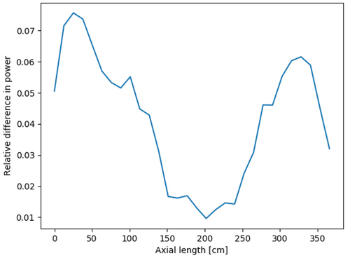
We then compare the behavior of the Frequency Transform method to the Adiabatic approximation in a fresh light water reactor fuel rod. The geometry is 365.76 cm long without spacer grids, undergoing a similar transient where the moderator density drops for 1 s and then rises again. The density change is uniform across the entire fuel rod. Since the Adiabatic approximation amounts to neglecting the time derivatives, it is considered less accurate than the Frequency Transform method. Figure 8 shows the relative difference in the axial power between the two methods at the end of the transient, with discrepancies as high as 7%. In this fuel rod model, the frequencies were calculated on a mesh with 30 axial cells and a single radial cell. Run parameters were 1 million particles per batch, 200 batches, including 100 inactive batches. Again, outer time steps are 0.5 s, inner time steps are 0.01 s, and outer time steps were forced to iterate twice.

Fig. 8. Axial power difference between the Frequency Transform and Adiabatic methods in a fuel rod after a 2-s transient.

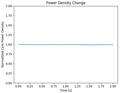
We also tested that this method holds steady state over 2 s on a fuel rod, as shown in Fig. 9. That is, the Frequency Transform method is applied, but no transient is prescribed. The maximum variation from steady power was found to be 1% and can be further decreased with larger numbers of particles. Considering the stochastic nature of the calculation, this is considered a successful steady state. These variations are tied directly to the neutron batch size, so lower neutron counts result in larger variations in the absence of feedback effects that can contribute to stability. These results were obtained with 1 million particles per batch over 200 batches with 100 inactive batches.

Fig. 9. Demonstration of holding steady state using the Frequency Transform method.

III.C. Evolution of Diffusion Parameters in Transient Calculations

In the formulation of this problem, the outer Monte Carlo time steps produce the multigroup parameters for TD-CMFD, including cross sections, diffusion coefficients, and cell-to-cell currents. Due to the approximations of diffusion theory, the currents calculated from diffusion are not guaranteed to match the currents tallied by Monte Carlo. Therefore, a nonlinear diffusion coupling term is introduced in CMFD to force equivalence with the Monte Carlo tallied currents.

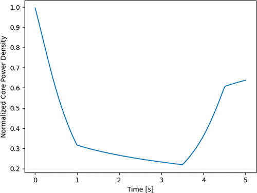
In many Monte Carlo applications for deterministic solvers, the multigroup parameters are generated at steady state for a given problem and used throughout the transient simulation. It is more accurate, however, to update the multigroup parameters throughout the transient, but the details on how often to do this and how to interpolate between these points is application-dependent. The use of TD-CMFD in this work presents a unique opportunity to observe the behavior of these parameters in a transient by studying the evolution of the values in time. In order to do so, we saved the values of linear and nonlinear diffusion terms, the total cross section, the absorption cross section (defined as the scattering cross section subtracted from the total cross section), and the downscattering cross section in select cells as calculated in our Frequency Transform method code in a fuel rod problem (with the same geometry and mesh as in Sec. III.B) using seven energy groups. Over the course of 5 seconds, the moderator density behaves as described in Table I. This results in a power profile shown in Fig. 10. Outer steps are 0.5 s, inner steps are 0.01 s, and outer time steps were forced to iterate twice. Run parameters are 400,000 particles per batch, with 1100 batches, including 100 inactive batches.

TABLE I Prescribed Evolution of Moderator Density During 5-s Transient Problem

Time Range (s)	Prescribed Behavior of Moderator Density Compared to Original Value
0–1.0	Linear drop to 80%
1.0–3.5	Remains at 80%
3.5–4.5	Linear rise to 100%
4.5–5.0	Remains at 100%

Fig. 10. Power profile for moderator density change transient.

For reporting the diffusion coefficients, we focused on the values on the off-diagonal of the CMFD matrix. These off-diagonal terms contain the linear diffusion coupling term and the nonlinear diffusion coupling term. The tallied diffusion coefficient in OpenMC uses a flux-limited transport correction. While there are better techniques in the literature for obtaining diffusion coefficients, only the flux-limited approximation is implemented in the main branch of OpenMC at this time.²⁴ Furthermore, the fuel rod geometry can be very well approximated by CMFD, so the nonlinear diffusion coefficients are expected to be nearly zero during this transient. The evolution of the cross sections will be more interesting for this particular geometry. Although no axial effects are expected due to the axial homogeneity of the transient, results are shown for cells at 1/3 and 2/3 of the height of the fuel rod to confirm this.

The behavior of the multigroup parameters are compared in time. Figures 11 and 12 present the linear and nonlinear diffusion terms, respectively, to show that the role of nonlinear diffusion coefficients is small in this problem, with fluctuations being primarily due to stochastic noise. Figures 13, 14, and 15 present several fast cross sections, which change in proportion to the moderator density. These cross sections are tallied at the outer time steps of 0.5 s and are linearly interpolated during the inner time steps.

Fig. 11. Linear diffusion terms in a cell at 1/3 and 2/3 height of the fuel rod.

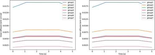
Fig. 12. Nonlinear diffusion terms in a cell at 1/3 and 2/3 height of the fuel rod.

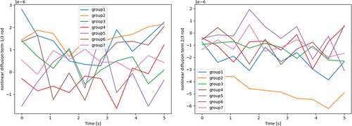
Fig. 13. Fastest-group total cross section in a cell at 1/3 and 2/3 height of the fuel rod.

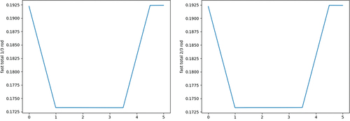
Fig. 14. Fastest-group absorption cross section in a cell at 1/3 and 2/3 height of the fuel rod.

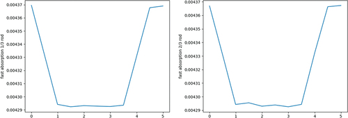
Fig. 15. Downscattering from the fastest group in a cell at 1/3 and 2/3 height of the fuel rod.

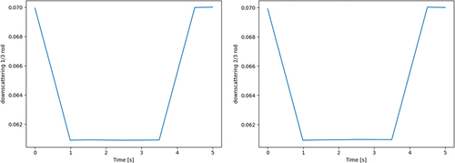
As expected, the nonlinear diffusion terms are very small in magnitude, suggesting that the linear diffusion coefficients alone sufficiently match the Monte Carlo currents in this problem. In fact, the diffusion coefficient is calculated based on transport, scattering, and flux tallies, which each have a relative error (defined as the standard deviation over the mean) of 0.14%, and the currents tallied to determine the nonlinear diffusion coefficients have a relative error of 0.67%. The magnitudes of the nonlinear diffusion terms therefore fall well within those uncertainties and are confirmed to have little effect in this problem. As for the cross sections, the lack of significant differences along the axial height of the fuel rod and the smooth lines shown across multiple outer time steps of 0.5 s suggest that the linear interpolation between these outer time steps is an adequate approximation for the simplicity of this transient. This is certainly not the case for all applications, as is well established in the rod-cusping problem or other similar transients with large heterogeneities.

IV. CONCLUSION

The Frequency Transform method applied to MC is a novel and efficient method for simulating transients on the order of a few seconds. The method relies on the approximation of the derivative terms in the time-dependent neutron transport equation by frequencies. These frequencies are calculated by TD-CMFD during inner time steps and are passed as inputs to MC during outer time steps. The results in this paper showed that the Frequency Transform method is more accurate than the Adiabatic approximation since the time derivatives are taken into account, and the spatial distribution of the frequencies provides additional information otherwise lacking in the Adiabatic method. One of the problems tested in this work showcased nonuniform changes in the geometry. By definition, the Frequency Transform method allows for such shape tilts thanks to the mesh on which frequencies are calculated.

Other than frequencies, many of the multigroup parameters can be used to track the transient and determine areas for improved simulation. The linear interpolation of cross sections between time steps is sufficient for a prescribed transient, as tested in this work, but may fall short in more sophisticated problems, such as a multiphysics implementation or an axially heterogeneous transient.

Acknowledgments

The first author was funded by the Department of Energy Computational Science Graduate Fellowship under grant DE-FG02-97ER25308. This research was also partially supported by the Exascale Computing Project (17-SC-20-SC), a collaborative effort of the U.S. Department of Energy (DOE) Office of Science and the National Nuclear Security Administration. This research made use of the resources of the High Performance Computing Center at Idaho National Laboratory, which is supported by the Office of Nuclear Energy of the DOE and the Nuclear Science User Facilities under contract number DE-AC07-05ID14517.

Disclosure Statement

No potential conflict of interest was reported by the author(s).

Additional information

Funding

This work was supported by the U.S. Department of Energy [DE-FG02-97ER25308]; U.S. Department of Energy [17-SC-20-SC].

References

- G. GRANDI, “SIMULATE3-K Models & Methodology,” SIMULATE3-K, Studsvik Scandpower (2011).
- S. SHANER, “Development of High Fidelity Methods for 3D Monte Carlo Analysis of Nuclear Reactors,” PhD Thesis, Massachusetts Institute of Technology (2018).
- B. BANDINI, “A Three-Dimensional Transient Neutronics Routine for the TRAC-PF1 Reactor Thermal Hydraulic Computer Code,” PhD Thesis, The Pennsylvania State University (1990).
- D. FERGUSON and K. HANSEN, “Solution of the Space-Dependent Reactor Kinetics Equations in Three Dimensions,” MIT-2903-4, U.S. Atomic Energy Commission Research and Development, Massachusetts Institute of Technology (1985).
- Y. CHAO and A. ATTARD, “A Resolution of the Stiffness Problem of Reactor Kinetics,” Nucl. Sci. Eng., 90, 1, 40 (1985); https://doi.org/10.13182/NSE85-A17429.
- Y. CHAO and P. HUANG, “Theory and Performance of the Fast-Running Multidimensional Pressurized Water Reactor Kinetics Code, SPNOVA-K,” Nucl. Sci. Eng., 103, 3, 415 (1989); https://doi.org/10.13182/NSE89-A23693.
- Y. BAN, T. ENDO, and A. YAMAMOTO, “A Unified Approach for Numerical Calculation of Space-Dependent Kinetic Equation,” J. Nucl. Sci. Technol., 49, 5, 496 (2012); https://doi.org/10.1080/00223131.2012.677126.
- J. Y. CHO et al., “Transient Capability for a MOC-Based Whole Core Transport Code DeCART,” Trans. Am. Nucl. Soc., 92, 721 (2005).
- M. KREHER, K. SMITH, and B. FORGET, “Direct Comparison of High-Order/Low-Order Transient Methods on the 2D-LRA Benchmark,” Nucl. Sci. Eng., 196, 409 (2022); https://doi.org/10.1080/00295639.2021.1980363.
- V. Y. GOL’DIN, G. V. DANILOVA, and B. N. CHETVERUSHKIN, “Approximate Method for Solving Time-Dependent Kinetic Equation,” Computational Methods in Transport Theory, Atomizdat, Moscow (1969).
- A. TAMANG and D. ANISTRATOV, “A Multilevel Projective Method for Solving the Space-Time Multigroup Neutron Kinetics Equations Coupled with the Heat Transfer Equation,” Nucl. Sci. Eng., 177, 1, 1 (2014); https://doi.org/10.13182/NSE13-42.
- P. GHASSEMI and D. ANISTRATOV, “An Approximation Method for Time-Dependent Problems in High Energy Density Thermal Radiative Transfer,” J. Comput. Theoret. Transp., 49, 31 (2020); https://doi.org/10.1080/23324309.2019.1709082.
- K. OTT, “Quasistatic Treatment of Spatial Phenomena in Reactor Dynamics,” Nucl. Sci. Eng., 26, 4, 563 (1966); https://doi.org/10.13182/NSE66-A18428.
- K. OTT and D. MENELEY, “Accuracy of the Quasistatic Treatment of Spatial Reactor Kinetics,” Nucl. Sci. Eng., 36, 402 (1969); https://doi.org/10.13182/NSE36-402.
- T. TRAHAN, “A Quasi-Static Monte Carlo Algorithm for the Simulation of Sub-Prompt Critical Transients,” Ann. Nucl. Energy, 127, 257 (2019); https://doi.org/10.1016/j.anucene.2018.11.055.
- C. BENTLEY, “Improvements in a Hybrid Stochastic/ Deterministic Method for Transient Three Dimensional Neutron Transport,” PhD Thesis, University of Tennessee Knoxville (1996).
- B. SJENITZER, “The Dynamic Monte Carlo Method for Transient Analysis of Nuclear Reactors,” PhD Thesis, Delft University of Technology (2014).
- V. VALTAVIRTA, M. HESSAN, and J. LEPPÄNEN, “Delayed Neutron Emission Model for Time Dependent Simulations with the SERPENT 2 Monte Carlo Code—First Results,” Proc. PHYSOR 2016, Sun Valley, Idaho, May 1–5, 2016, American Nuclear Society (2016).
- D. FERRARO et al., “SERPENT and TRIPOLI-4 Transient Calculations Comparisons for Several Reactivity Insertion Scenarios in a 3D Minicore Benchmark,” Proc. Int. Conf. Mathematics and Computational Methods Applied to Nuclear Science and Engineering (M&C2019), Portland, Oregon, August 25–29, 2019, American Nuclear Society (2019).
- M. FAUCHER, D. MANCUSI, and A. ZOIA, “New Kinetic Simulation Capabilities for TRIPOLI-4: Methods and Applications,” Ann. Nucl. Energy, 120, 74 (2018); https://doi.org/10.1016/j.anucene.2018.05.030.
- D. CULLEN, “Tart 2002: A Coupled Neutron-Photon, 3D, Combinatorial Geometry, Time Dependent Monte Carlo Transport Code,” UCRL-ID-126455, Lawrence Livermore National Laboratory (2002).
- P. ROMANO et al., “OpenMC: A State-of-the-Art Monte Carlo Code for Research and Development,” Ann. Nucl. Energy, 82, 90 (2015); https://doi.org/10.1016/j.anucene.2014.07.048.
- J. HOU et al., “OECD/NEA Benchmarks for Time-Dependent Neutron Transport Calculations Without Spatial Homogenization,” Nucl. Eng. Des., 317, 177 (2017); https://doi.org/10.1016/j.nucengdes.2017.02.008.
- Z. LIU et al., “Cumulative Migration Method for Computing Rigorous Diffusion Coefficients and Transport Cross Sections from Monte Carlo,” Ann. Nucl. Energy, 112, 507 (2018); https://doi.org/10.1016/j.anucene.2017.10.039.