An Inline Burnup Algorithm

Abstract

Inline algorithms have been proposed for coupling Monte Carlo neutron transport solvers with several other physics, such as xenon and iodine densities and thermal hydraulics. This paper proposes a new inline algorithm that can be applied to burnup calculations. The algorithm is a modification of the predictor-corrector method, where the corrector-step nuclide densities are converged simultaneously with the fission source. This could, in principle, obviate the need for two full neutronics solutions per time-step while still allowing the accuracy of predictor-corrector methods with improved stability. This paper describes the algorithm and demonstrates its stability properties through a Fourier analysis. Although not unconditionally stable, judicious use of batching and relaxation are shown to greatly improve the algorithm’s stability properties in realistic systems.

Keywords:

• Neutronics
• burnup
• stability
• Monte Carlo

I. INTRODUCTION

Monte Carlo neutron transport solvers are increasingly common in research and in industry for resolving the neutronic behavior of nuclear reactor cores. This has been enabled by a swell in the availability of computing power over time. Although it is now conceivable to resolve neutronics in isolation, the computational expense of Monte Carlo solvers is such that coupling it with other important physics, such as thermal hydraulics or fuel mechanics, remains challenging due to the need to perform several Monte Carlo calculations to achieve convergence between the solvers. This common strategy for handling multiphysics calculations is known as fixed-point iteration.

Inline algorithms have recently become popular as a means of avoiding the computational expense of fixed-point iteration in converging neutronics with other physics. The logic of such algorithms is that they iteratively pass information from the Monte Carlo solver to the other physics solvers during Monte Carlo’s inactive cycles, i.e., before the neutronics solution is fully converged. These other physics solvers then update the macroscopic cross sections in the neutronics problem (either by modifying densities or temperatures) and the inactive cycles continue with this periodic data exchange. This makes intuitive sense in that it is undesirable to fully converge a neutronics solution when (due to inevitable changes in other physics) the macroscopic cross sections that describe the geometry are known to be erroneous. This strategy has been applied to converging Monte Carlo with xenon,¹ thermal hydraulics,^2,3 and with both simultaneously.⁴ Analogous strategies are used and described in coupling deterministic transport with other physics, with the accompanying analysis highlighting the additional numerical stability and convergence acceleration that this provides.^5–10

Isotopic depletion, or burnup, is another vital component of reactor physics, governing a reactor’s cycle length, the evolution of its power profile, and its spent fuel inventory, among other quantities of interest. The natural coupling between neutronics and depletion has neutronics generating reaction rates that the depletion solver uses to evolve the geometry’s isotopic composition forward by some chosen time step. Additional sophistication can occur, such as storing and using multiple transport solutions across several time steps to increase the order of accuracy of the time-stepping schemes. This is where much of the work on coupling neutronics and depletion has been to date.^11–14 Again, due to the expense of the Monte Carlo solution, it is desirable to minimize the number of neutronics solutions that must be found when considering the depletion of a reactor geometry.

In larger geometries, however, it has been found that numerical instability can also result from this coupling between neutronics and depletion.^15–19 This spurious behavior can often be avoided by removing the particularly troublesome depletion chain of ¹³⁵Xe from the system and converging its nuclide density distribution separately,²⁰ although this is no guarantee of unconditional stability. Other means of ensuring stability introduce the equivalent of an implicit time-stepping scheme, where an iteration takes place between neutronics and depletion, invariably with some form of relaxation.^19,21–26 Such schemes unfortunately impose additional undesirable computational expense.

Given the numerical stability and relatively low computational expense of other inline algorithms, it appears natural to propose applying it to depletion to overcome the drawbacks of the current implicit methods. To the authors’ knowledge, this was first proposed in the literature by Cosgrove,²⁷ although a version of the algorithm has actually existed in the Serpent Monte Carlo code as of version 2.1.31, albeit of a slightly different implementation than is considered here.²⁸

This paper will first describe the inline algorithm before performing a stability analysis to demonstrate its beneficial numerical properties.

II. BURNUP ALGORITHMS

Before describing the new algorithm, a brief discussion of the basics of neutronics-depletion coupling is warranted.

Neutronics is governed by the neutron transport equation. In reactor analysis, this tends to be the eigenvalue form of the transport equation:

(1) $\begin{array}{c}\mathbf{\Omega }\cdot \mathrm{\nabla }\psi +{\mathrm{\Sigma }}_{\mathrm{t}}\psi =\frac{\chi }{4\pi k}{\int }_0^{\mathrm{\infty }}\mathrm{d}E{ }^{\mathrm{\prime }}\nu {\mathrm{\Sigma }}_{\mathrm{f}}{\int }_{4\pi }\mathrm{d}\mathbf{\Omega }{ }^{\mathrm{\prime }}\psi +{\int }_0^{\mathrm{\infty }}\mathrm{d}E{ }^{\mathrm{\prime }}{\int }_{4\pi }\mathrm{d}\mathbf{\Omega }{ }^{\mathrm{\prime }}{\mathrm{\Sigma }}_{\mathrm{s}}(E{ }^{\mathrm{\prime }}\to E,\mathbf{\Omega }{ }^{\mathrm{\prime }}\to \mathbf{\Omega })\psi ,\end{array}$(1)

where

$\mathbf{\Omega }$ =	=	neutron direction of flight
$\psi$ =	=	angular neutron flux
${\mathrm{\Sigma }}_r,r\in \{\mathrm{t},\mathrm{f},\mathrm{s}\}$ =	=	macroscopic cross sections for the total, fission, and scattering reactions
$\chi$ =	=	fission neutron energy spectrum
$k$ =	=	criticality eigenvalue
$E$ =	=	neutron energy
$\nu$ =	=	average number of neutrons produced per fission.

As well as the eigenvalue, the quantities of interest from the solution of the transport equation tend to be the reaction rates of neutrons with isotopes present in the system, either as a whole or over some particular volume. These are microscopic reaction rates averaged over a given volume of space of uniform composition where depletion calculations are concerned:

(2) $⟨{\sigma }_r,\psi ⟩=\frac{1}{V}{\int }_0^{\mathrm{\infty }}\mathrm{d}E{\sigma }_r{\int }_{4\pi }\mathrm{d}\mathbf{\Omega }{\int }_V\mathrm{d}V\psi ,$(2)

where ${\sigma }_r$ is the microscopic cross section for reaction channel $r$, and $V$ is the volume of space of interest. Instead of obtaining microscopic reaction rates, neutronics codes may obtain one-group microscopic cross sections and flux amplitudes that can be multiplied together to recover Eq. (2):

(3a) $⟨{\sigma }_r⟩=\frac{{\int }_0^{\mathrm{\infty }}\mathrm{d}E{\sigma }_r{\int }_{4\pi }\mathrm{d}\mathbf{\Omega }{\int }_V\mathrm{d}V\psi }{{\int }_0^{\mathrm{\infty }}\mathrm{d}E{\int }_{4\pi }\mathrm{d}\mathbf{\Omega }{\int }_V\mathrm{d}V\psi }$(3a)

and

(3b) $⟨\psi ⟩=\frac{1}{V}{\int }_0^{\mathrm{\infty }}\mathrm{d}E{\int }_{4\pi }\mathrm{d}\mathbf{\Omega }{\int }_V\mathrm{d}V\psi .$(3b)

The evolution of the density of a nuclide with index $i$, $N_i$, with time $t$ is given as

(4) $\frac{\mathrm{d}{N}_i}{\mathrm{d}t}=\sum _j\left[⟨{\gamma }^{ij}{\sigma }_{\mathrm{f}},\psi ⟩+⟨l^{ij}{\sigma }_{\mathrm{c}},\psi ⟩+{\lambda }^{ij}-{\delta }_{ij}({\lambda }^j+⟨{\sigma }_{\mathrm{a}},\psi ⟩)\right]N_j,$(4)

where

${\gamma }^{ij}$ =	=	fission yield of nuclide $i$ on fissioning nuclide $j$
$l^{ij}$ =	=	branching ratio producing nuclide $i$ when nuclide $j$ undergoes neutron capture
${\lambda }^{ij}$ =	=	decay constant for nuclide $j$ decaying into nuclide $i$
${\delta }_{ij}$ =	=	Kronecker delta.

For a system of nuclides (fission reactor neutronics/depletion tools tend to track at least hundreds^29,30), one has the Bateman equation governing their evolution³¹:

(5) $\frac{\mathrm{d}N}{\mathrm{d}t}=\mathbf{A}N,$(5)

where $N$ is now a vector of nuclides and $\mathbf{A}$ is the burnup matrix with the element ${\mathbf{A}}_{ij}$ describing the production or loss terms of nuclide $i$ from nuclide $j$. The formal solution of the Bateman equation for a constant burnup matrix after a time step of length $\mathrm{\Delta }t$ from an initial nuclide density $N_0$ is the matrix exponential:

(6) $N(\mathrm{\Delta }t)=exp(\mathrm{\Delta }t\mathbf{A})N_0.$(6)

Evaluating this matrix exponential is difficult,³² although for burnup matrices this can be accurately done using the Chebyshev rational approximation method^33,34 (CRAM). Other accurate methods of solving the Bateman equation include using more familiar Ordinary Differential Equation (ODE) solvers.^29,35 The Bateman equation is valid in a homogeneous region, whereas in reactor problems, one is generally interested in how the many different regions of the problem evolve. Thus burnup problems tend to discretize the reactor geometry into many separate, homogeneous burnable regions in which reaction rates are obtained and where the Bateman equation is solved separately. For large, finely discretized reactor geometries, this may impose a substantial computer memory burden unless care is taken.²⁹ Although relatively unexplored, a spatially continuous approach to depletion has also been proposed and preliminarily investigated.³⁶

The fundamental problem in numerical burnup calculations is that the burnup matrix is not constant in time. It is a function of the neutron flux, which is itself dependent upon the evolving nuclide density distribution in the system through the macroscopic cross sections appearing in Eq. (1)(1) $\begin{array}{c}\mathbf{\Omega }\cdot \mathrm{\nabla }\psi +{\mathrm{\Sigma }}_{\mathrm{t}}\psi =\frac{\chi }{4\pi k}{\int }_0^{\mathrm{\infty }}\mathrm{d}E{ }^{\mathrm{\prime }}\nu {\mathrm{\Sigma }}_{\mathrm{f}}{\int }_{4\pi }\mathrm{d}\mathbf{\Omega }{ }^{\mathrm{\prime }}\psi +{\int }_0^{\mathrm{\infty }}\mathrm{d}E{ }^{\mathrm{\prime }}{\int }_{4\pi }\mathrm{d}\mathbf{\Omega }{ }^{\mathrm{\prime }}{\mathrm{\Sigma }}_{\mathrm{s}}(E{ }^{\mathrm{\prime }}\to E,\mathbf{\Omega }{ }^{\mathrm{\prime }}\to \mathbf{\Omega })\psi ,\end{array}$(1) . That is,

(7) $\frac{\mathrm{d}N}{\mathrm{d}t}=\mathbf{A}(\psi )N.$(7)

Thus, the burnup problem is nonlinear.

The simplest approach to coupling neutronics and depletion and resolving this nonlinearity is the explicit Euler method (sometimes known as the predictor method). Following a neutronics solution and obtaining microscopic reaction rates across the geometry, the Bateman equation is evaluated for each region for a chosen time-step length $\mathrm{\Delta }t$ and the process is repeated until the end of the depletion period of interest As well as possessing a low order of accuracy, necessitating short time steps, the explicit Euler scheme is only conditionally stable, even for simple systems.¹⁸

A slightly more sophisticated time-stepping algorithm is the predictor-corrector method, which enjoys a higher-order accuracy in time.¹⁴ There are several variants of this scheme with slightly different properties; here we consider what Isotalo refers to as the Constant Extrapolation/Linear Interpolation (CE/LI) method implemented in Serpent,²⁸ MC21 (Ref. 37), and OpenMC (Ref. 30). This begins with the explicit Euler method, where neutronics is evaluated at some time point with index $n$, known as the beginning of step or BOS, and the resulting burnup matrix ${\mathbf{A}}_n$ is used to generate a nuclide density distribution at a time point with index $n+1$ at $\mathrm{\Delta }t$ in the future, known as the end of step or EOS. This is the predictor step, with its depletion described by the following equation:

(8) $N_{n+1}=exp\left(\mathrm{\Delta }t{\mathbf{A}}_n\right)N_n.$(8)

Another neutronics solution is evaluated at this future time and reaction rates are obtained, allowing for the construction of a second burnup matrix ${\mathbf{A}}_{n+1}$. Finally, depletion is performed again to generate the nuclide density distribution to be used at the next time step, but using a time-averaged burnup matrix:

(9) $N_{n+1}=exp\left(\mathrm{\Delta }t\frac{{\mathbf{A}}_n+{\mathbf{A}}_{n+1}}{2}\right)N_n.$(9)

The CE/LI method is shown in Algorithm 1. In the algorithm, $\psi (N_n)$ denotes the evaluation of a transport solution given the nuclide density distribution $N_n$. Unfortunately, the predictor-corrector method, too, is only conditionally stable for simple systems,^16,17,19 necessitating a workaround such as handling xenon separately²⁰ or implicit methods.

Algorithm 1: Predictor-Corrector Method

Input: $N_0,n_{\mathrm{s}\mathrm{t}\mathrm{e}\mathrm{p}\mathrm{s}},\mathrm{\Delta }t$

for $n=0,\dots ,n_{\mathrm{s}\mathrm{t}\mathrm{e}\mathrm{p}\mathrm{s}}-1$ do

 | /* Evaluate BOS transport solution      */

 | ${\mathrm{A}}_n\leftarrow$ ψ $\left(N_n\right)$

 | /* Perform predictor depletion        */

 | $N_{n+1}\leftarrow exp[{\mathrm{A}}_n\mathrm{\Delta }{t}_n]N_n$

 | /* Evaluate EOS transport solution      */

 | ${\mathrm{A}}_{n+1}\leftarrow$ ψ $(N_{n+1})$

 | $\mathrm{A}\leftarrow \frac{1}{2}\left({\mathrm{A}}_n+{\mathrm{A}}_{n+1}\right)$

 | /* Perform corrector depletion        */

 | |$N_{n+1}\leftarrow exp[\mathrm{A}\mathrm{\Delta }{t}_n]N_n$

end

 | |||

All implicit methods work by iterating between neutronics and depletion at the EOS, each of which includes an under relaxation to stabilize the iteration, which is applied either to the reaction rates or the nuclide densities. The first of these was the Stochastic Implicit Euler (SIE) method,²¹ although it is more akin to a backward Euler method due to iterating with only the EOS burnup matrix. This results in it only being first-order accurate. The stochastic in SIE comes from using the Stochastic Approximation to decide the relaxation factor applied.³⁸ A higher-order method that is equivalent to an implicit CE/LI scheme is the Stochastic Implicit Midpoint method.²² This method begins with a slightly modified version of Eq. (8)(8) $N_{n+1}=exp\left(\mathrm{\Delta }t{\mathbf{A}}_n\right)N_n.$(8) :

(10) $N_{n+1}^{(0)}=exp\left(\mathrm{\Delta }t{\mathbf{A}}_n\right)N_n,$(10)

where $N_{n+1}^{(0)}$ is the initial $n+1$’th nuclide density vector to begin the fixed-point iteration. On the $j+1$’th iteration, a transport solution is evaluated from $N_{n+1}^{(j)}$ to generate the corresponding burnup matrix ${\mathbf{A}}_{n+1}^{(j)}$. This is then used in the following corrector depletion equation:

(11) $N_{n+1}^{(j+1)}={\alpha }_{j}exp\left(\mathrm{\Delta }t\frac{{\mathbf{A}}_n+{\mathbf{A}}_{n+1}^{(j)}}{2}\right)N_n+(1-{\alpha }_j)N_{n+1}^{(j)},$(11)

where ${\alpha }_j$ is the relaxation factor, which may vary with the iteration or remain constant.²⁶ Higher-order implicit methods have also been described, where the predictor and corrector depletion calculations use additional information from previous transport solutions and divide the depletion interval into substeps where the coefficients in front of the burnup matrices are varied.^23–25 The implicit mid-point scheme is shown in Algorithm 2.

Algorithm 2: Implicit Midpoint Method

 Input: $N_0,n_{\mathrm{s}\mathrm{t}\mathrm{e}\mathrm{p}\mathrm{s}},\mathrm{\Delta }t,j_{max},\alpha$

 for $n=0,\dots ,n_{\mathrm{s}\mathrm{t}\mathrm{e}\mathrm{p}\mathrm{s}}-1\mathbf{d}\mathbf{o}$

   /* Evaluate BOS transport solution */

   $A_n\leftarrow \psi \left(N_n\right)$

   /* Perform predictor depletion */

   $N_{n+1}^{(0)}\leftarrow exp\left[{\mathrm{A}}_n\mathrm{\Delta }{t}_n\right]N_n$

   /* Iterate on the corrector step */

   for $j=0,\dots ,j_{max}-1\mathbf{d}\mathbf{o}$

     /* Evaluate EOS transport solution */

     $A_{n+1}^{\left(j\right)}\leftarrow \psi \left(N_{n+1}^{\left(j\right)}\right)$

     $\mathrm{A}\leftarrow \frac{1}{2}\left({\mathrm{A}}_n+{\mathrm{A}}_{n+1}^{\left(j\right)}\right)$

     /* Perform corrector depletion with relaxation */

     $N_{n+1}^{\left(j+1\right)}\leftarrow {\alpha }_{j}exp\left[\mathrm{A}\mathrm{\Delta }{t}_n\right]N_n+\left(1-{\alpha }_j\right)N_{n+1}^{\left(j\right)}$

   end

     $N_{n+1}\leftarrow N_{n+1}^{\left(j_{max}\right)}$

 end

Inline algorithms efficiently converge a nonlinearity between neutronics and other physics; in depletion, that nonlinearity is normally handled during the fixed-point iteration on the corrector step, corresponding to Eq. (11)(11) $N_{n+1}^{(j+1)}={\alpha }_{j}exp\left(\mathrm{\Delta }t\frac{{\mathbf{A}}_n+{\mathbf{A}}_{n+1}^{(j)}}{2}\right)N_n+(1-{\alpha }_j)N_{n+1}^{(j)},$(11) . The proposed inline algorithm, as with all of the previous depletion algorithms, begins with a standard predictor step to generate the initial EOS nuclide density vector, corresponding to Eq. (10)(10) $N_{n+1}^{(0)}=exp\left(\mathrm{\Delta }t{\mathbf{A}}_n\right)N_n,$(10) . During one or several inactive cycles, denoted with index $c$, of the EOS neutronics, reaction rates are scored to construct a burnup matrix for each burnable region ${\mathbf{A}}_{n+1}^{(c)}$. At the conclusion of this batch of cycles, the nuclide density vectors in each region are updated according to

(12) $N_{n+1}^{(c)}=exp\left(\mathrm{\Delta }t\frac{{\mathbf{A}}_n+{\mathbf{A}}_{n+1}^{(c)}}{2}\right)N_n.$(12)

Provided the effects of statistical noise are not deleterious, this iteration should hopefully converge the corrector neutronics and densities, as occurs with thermal hydraulics and xenon. As with other implicit methods in burnup calculations, this corrector could be replaced with higher-order versions using substepping and quadratic interpolation. In principle, if convergence is reached, the active cycles of the EOS could be foregone entirely; a single transport solution could act as the BOS solution during the active cycles and as the EOS during the inactive. The only exception to this is during the first transport solution where the fission source must be converged before scoring reaction rates for the predictor. The inline scheme is shown in Algorithm 3. In this algorithm, $V$ has been included as an input to more explicitly account for the geometry and the uniform sampling of the initial fission source across the geometry, shown as $F^{(0)}\leftarrow \mathrm{u}\mathrm{n}\mathrm{i}\mathrm{f}(V)$. In principle, other tallying strategies might be used, other than accumulating tallies across several batches before flushing them and beginning anew. For example, one might employ the moving-window approach suggested by Ref. 3 where the corrector update is performed every cycle but using reaction rates accumulated over several previous cycles.

Algorithm 3: Inline Predictor-Corrector Algorithm

Input: $N_0,n_{\mathrm{s}\mathrm{t}\mathrm{e}\mathrm{p}\mathrm{s}},\mathrm{\Delta }t,n_{\mathrm{i}\mathrm{n}\mathrm{a}\mathrm{c}\mathrm{t}\mathrm{i}\mathrm{v}\mathrm{e}},n_{\mathrm{a}\mathrm{c}\mathrm{t}\mathrm{i}\mathrm{v}\mathrm{e}},V$

for $n=0,\dots ,n_{steps}-1$ do

  if $n=0$ then

    /* The initial BOS neutronics calculation has no feedback */

    $\left[{\mathcal{L}}_n,v\sum _{f,n}\right]\leftarrow N_0$

    ${\kappa }^{\left(0\right)}\leftarrow 1$

    $F^{\left(0\right)}\leftarrow \mathrm{u}\mathrm{n}\mathrm{i}\mathrm{f}\left(V\right)$

    for $c=0,\dots ,n_{\mathrm{i}\mathrm{n}\mathrm{a}\mathrm{c}\mathrm{t}\mathrm{i}\mathrm{v}\mathrm{e}}-1$ do

      ${\psi }^{\left(c+1\right)}\leftarrow \frac{1}{{\kappa }^{\left(c\right)}}{\left({\mathcal{L}}_n\right)}^{-1}{F}^{(c)}$

      $F^{\left(c+1\right)}\leftarrow \int \hspace{0.17em}\int v\sum _{\mathrm{f},n}{\psi }^{\left(c+1\right)}\mathrm{d}\mathrm{\Omega }\mathrm{d}E$

      ${\kappa }^{\left(c+1\right)}\leftarrow {\kappa }^{\left(c\right)}\frac{\int \hspace{0.17em}{F}^{\left(c+1\right)}\mathrm{d}V}{\int \hspace{0.17em}{F}^{\left(c\right)}\mathrm{d}V}$

    end

  else

    /* Converge neutronics with nonlinear feedback during EOS */

    ${\kappa }^{\left(0\right)}\leftarrow 1$

    $F^{\left(0\right)}\leftarrow \mathrm{u}\mathrm{n}\mathrm{i}\mathrm{f}\left(V\right)$

    ${\mathrm{A}}_n\leftarrow \mathrm{\Lambda }$

    for $c=0,\dots ,n_{\mathrm{i}\mathrm{n}\mathrm{a}\mathrm{c}\mathrm{t}\mathrm{i}\mathrm{v}\mathrm{e}}-1$ do

      ${\psi }^{\left(c+1\right)}\leftarrow \frac{1}{{\kappa }^{\left(c\right)}}{\left({\mathcal{L}}^{\left(c\right)}\right)}^{-1}{F}^{\left(c\right)}$

      $F^{\left(c+1\right)}\leftarrow \int \hspace{0.17em}\int v\sum _{\mathrm{f},n}^{(c)}{\psi }^{\left(c+1\right)}\mathrm{d}\mathrm{\Omega }\mathrm{d}E$

      ${\kappa }^{\left(c+1\right)}\leftarrow {\kappa }^{\left(c\right)}\frac{\int \hspace{0.17em}{F}^{\left(c+1\right)}\mathrm{d}V}{\int \hspace{0.17em}{F}^{\left(c\right)}\mathrm{d}V}$

      ${\mathrm{A}}_n+=⟨\sigma ,{\psi }^{\left(c+1\right)}⟩$

      $\mathrm{A}\leftarrow \frac{1}{2}\left({\mathrm{A}}_{n-1}+{\mathrm{A}}_n\right)$

      $N_n^{\left(c+1\right)}\leftarrow exp\left[\mathrm{A}\mathrm{\Delta }{t}_{n-1}\right]N_{n-1}$

      $\left[{\mathcal{L}}_n^{\left(c+1\right)},v{\mathrm{\Sigma }}_{f,n}^{\left(c+1\right)}\right]\leftarrow N_n^{\left(c+1\right)}$

      ${\mathrm{A}}_n\leftarrow \mathrm{\Lambda }$

    end

    $N_n\leftarrow N_n^{\left(c+1\right)}$

    $\left[{\mathcal{L}}_n,v{\mathrm{\Sigma }}_{\mathrm{f},n}\right]\leftarrow \left[{\mathcal{L}}_n^{\left(c+1\right)},v{\mathrm{\Sigma }}_{\mathrm{f},n}^{\left(c+1\right)}\right]$

  end

  /* Generate BOS burn-up matrix during active cycles */

  ${\mathrm{A}}_n\leftarrow \mathrm{\Lambda }$

  for $c=0,\dots ,n_{\mathrm{a}\mathrm{c}\mathrm{t}\mathrm{i}\mathrm{v}\mathrm{e}}-1$ do

    ${\psi }^{\left(c+1\right)}\leftarrow \frac{1}{{\kappa }^{\left(c\right)}}{\left({\mathcal{L}}_n\right)}^{-1}{F}^{(c)}$

    ${\mathrm{A}}_n+=⟨\sigma ,{\psi }^{\left(c+1\right)}⟩$

    $F^{\left(c+1\right)}\leftarrow \int \hspace{0.17em}\int v\sum _{\mathrm{f},n}{\psi }^{\left(c+1\right)}\mathrm{d}\mathrm{\Omega }\mathrm{d}E$

    ${\kappa }^{\left(c+1\right)}\leftarrow {\kappa }^{\left(c\right)}\frac{\int \hspace{0.17em}{F}^{\left(c+1\right)}\mathrm{d}V}{\int \hspace{0.17em}{F}^{\left(c\right)}\mathrm{d}V}$

  end

  $N_{n+1}\leftarrow exp\left[{\mathrm{A}}_n\mathrm{\Delta }{t}_n\right]N_n$

end

III. STABILITY ANALYSIS

The inline depletion scheme is now sufficiently defined to permit a stability analysis. A stability analysis (or Fourier or Von Neumann stability analysis) is used to analyze the behavior of iterative methods or time-stepping schemes across computational physics. Where neutronics and depletion are concerned, several papers on stability analysis have been published to date^{18,19,39–41} and the analysis to follow descends directly from them.

A stability analysis consists of, first, applying the equations describing the numerical method to a simple system where their behavior can be determined analytically. The solution of the system on iteration or evolution in time may then be expressed in terms of this known initial solution plus perturbation terms. Provided the system is sufficiently simple, these perturbation terms can be decomposed into Fourier modes. By linearizing the governing equations, one can obtain expressions for how the Fourier modes during one time step are related to those at the next, either by a scalar or matrix. The magnitude of the scalar or the spectral radius of the matrix determines the behavior of a particular Fourier mode across time steps; if this value is greater than one, then that Fourier mode will grow. Growth in a particular Fourier mode implies that the given algorithm is numerically unstable.

The equations used for the inline scheme must be chosen. These are those describing neutronics, predictor depletion, and corrector depletion. For neutronics, rather than Eq. (1(1) $\begin{array}{c}\mathbf{\Omega }\cdot \mathrm{\nabla }\psi +{\mathrm{\Sigma }}_{\mathrm{t}}\psi =\frac{\chi }{4\pi k}{\int }_0^{\mathrm{\infty }}\mathrm{d}E{ }^{\mathrm{\prime }}\nu {\mathrm{\Sigma }}_{\mathrm{f}}{\int }_{4\pi }\mathrm{d}\mathbf{\Omega }{ }^{\mathrm{\prime }}\psi +{\int }_0^{\mathrm{\infty }}\mathrm{d}E{ }^{\mathrm{\prime }}{\int }_{4\pi }\mathrm{d}\mathbf{\Omega }{ }^{\mathrm{\prime }}{\mathrm{\Sigma }}_{\mathrm{s}}(E{ }^{\mathrm{\prime }}\to E,\mathbf{\Omega }{ }^{\mathrm{\prime }}\to \mathbf{\Omega })\psi ,\end{array}$(1) ), the one-dimensional, monoenergetic, neutron diffusion equation in slab geometry will be used in $k$-eigenvalue form, assuming isotropic scattering:

(13) $\left(-\frac{\mathrm{\partial }}{\mathrm{\partial }x}D\frac{\mathrm{\partial }}{\mathrm{\partial }x}+{\mathrm{\Sigma }}_{\mathrm{a}}\right)\varphi =\frac{1}{k}\nu {\mathrm{\Sigma }}_{\mathrm{f}}\varphi ,$(13)

where

$x\in [0,L]$ =	=	spatial variable across a domain of length $L$
$D$ =	=	neutron diffusion coefficient
${\mathrm{\Sigma }}_{\mathrm{a}}$ =	=	macroscopic absorption cross section
$\varphi$ =	=	scalar neutron flux
$\nu$ =	=	average number of neutrons per fission
${\mathrm{\Sigma }}_{\mathrm{f}}$ =	=	macroscopic fission cross section
$k$ =	=	criticality eigenvalue.

Provided there is no leakage, the criticality eigenvalue is defined as

(14) $k=\frac{{\int }_0^L\nu {\mathrm{\Sigma }}_{\mathrm{f}}\varphi \mathrm{d}x}{{\int }_0^L{\mathrm{\Sigma }}_{\mathrm{a}}\varphi \mathrm{d}x}.$(14)

This expression for $k$ becomes slightly more complicated when accounting for how the flux and composition (in our particular circumstances) evolve during the source iterations. Including the dependence of both on the source iteration index $c$, this becomes

(15) $k^{(c)}=\frac{{\int }_0^L\nu {\mathrm{\Sigma }}_{\mathrm{f}}^{(c-1)}{\varphi }^{(c)}\mathrm{d}x}{{\int }_0^L{\mathrm{\Sigma }}_{\mathrm{a}}^{(c-1)}{\varphi }^{(c)}\mathrm{d}x}.$(15)

The approximations applied in going from Eq. (1)(1) $\begin{array}{c}\mathbf{\Omega }\cdot \mathrm{\nabla }\psi +{\mathrm{\Sigma }}_{\mathrm{t}}\psi =\frac{\chi }{4\pi k}{\int }_0^{\mathrm{\infty }}\mathrm{d}E{ }^{\mathrm{\prime }}\nu {\mathrm{\Sigma }}_{\mathrm{f}}{\int }_{4\pi }\mathrm{d}\mathbf{\Omega }{ }^{\mathrm{\prime }}\psi +{\int }_0^{\mathrm{\infty }}\mathrm{d}E{ }^{\mathrm{\prime }}{\int }_{4\pi }\mathrm{d}\mathbf{\Omega }{ }^{\mathrm{\prime }}{\mathrm{\Sigma }}_{\mathrm{s}}(E{ }^{\mathrm{\prime }}\to E,\mathbf{\Omega }{ }^{\mathrm{\prime }}\to \mathbf{\Omega })\psi ,\end{array}$(1) to Eq. (13)(13) $\left(-\frac{\mathrm{\partial }}{\mathrm{\partial }x}D\frac{\mathrm{\partial }}{\mathrm{\partial }x}+{\mathrm{\Sigma }}_{\mathrm{a}}\right)\varphi =\frac{1}{k}\nu {\mathrm{\Sigma }}_{\mathrm{f}}\varphi ,$(13) are quite severe. Some of these are justifiable. Problems in which depletion instabilities occur tend to be large thermal systems dominated by scattering where the diffusion approximation is reasonable, indeed a transport equation can be used instead, but no substantial differences have been observed in problems considered so far.³⁹ This is expected, given that numerical instabilities in burnup arise from the low-frequency Fourier modes and transport and diffusion agree in the low-frequency limit.

As scattering is isotropic, the diffusion coefficient in Eq. (13)(13) $\left(-\frac{\mathrm{\partial }}{\mathrm{\partial }x}D\frac{\mathrm{\partial }}{\mathrm{\partial }x}+{\mathrm{\Sigma }}_{\mathrm{a}}\right)\varphi =\frac{1}{k}\nu {\mathrm{\Sigma }}_{\mathrm{f}}\varphi ,$(13) is

(16) $D=\frac{1}{3{\mathrm{\Sigma }}_{\mathrm{t}}}.$(16)

The cross sections featured in Eq. (13(13) $\left(-\frac{\mathrm{\partial }}{\mathrm{\partial }x}D\frac{\mathrm{\partial }}{\mathrm{\partial }x}+{\mathrm{\Sigma }}_{\mathrm{a}}\right)\varphi =\frac{1}{k}\nu {\mathrm{\Sigma }}_{\mathrm{f}}\varphi ,$(13) ) are the inner product of the nuclide density vector (which is taken to be continuous in $x$) and the corresponding microscopic cross-section vector, such that

(17a) ${\mathrm{\Sigma }}_{\mathrm{a}}={\sigma }_{\mathrm{a}}^{\mathrm{T}}N,$(17a)

(17b) ${\mathrm{\Sigma }}_{\mathrm{t}}={\sigma }_{\mathrm{t}}^{\mathrm{T}}N,$(17b)

and

(17c) $\nu {\mathrm{\Sigma }}_{\mathrm{f}}=(\nu {\sigma }_{\mathrm{f}}{)}^{\mathrm{T}}N.$(17c)

Equation (13)(13) $\left(-\frac{\mathrm{\partial }}{\mathrm{\partial }x}D\frac{\mathrm{\partial }}{\mathrm{\partial }x}+{\mathrm{\Sigma }}_{\mathrm{a}}\right)\varphi =\frac{1}{k}\nu {\mathrm{\Sigma }}_{\mathrm{f}}\varphi ,$(13) requires a normalization condition to determine the amplitude of the neutron flux; reactor power is a common choice in depletion calculations. In one dimension, this normalization would be to a fixed power per unit area $P$ such that

(18) $P={\int }_0^L\kappa {\mathrm{\Sigma }}_{\mathrm{f}}\varphi \mathrm{d}x,$(18)

where $\kappa$ is the average energy release per fission. One must also specify boundary conditions for Eq. (13)(13) $\left(-\frac{\mathrm{\partial }}{\mathrm{\partial }x}D\frac{\mathrm{\partial }}{\mathrm{\partial }x}+{\mathrm{\Sigma }}_{\mathrm{a}}\right)\varphi =\frac{1}{k}\nu {\mathrm{\Sigma }}_{\mathrm{f}}\varphi ,$(13) . These may be either reflective or periodic to enable the subsequent Fourier decomposition, with the choice determining the allowable Fourier frequencies.

Two slightly different versions of the diffusion equation feature in the following analysis, accounting for both the change in macroscopic cross sections during burnup and for the equation’s solution method. First, when solving the diffusion equation to full convergence at time point $n$, it may be written as

(19) $\left(-\frac{\mathrm{\partial }}{\mathrm{\partial }x}{D}_n\frac{\mathrm{\partial }}{\mathrm{\partial }x}+{\mathrm{\Sigma }}_{\mathrm{a},n}\right){\varphi }_n=\frac{1}{k_n}\nu {\mathrm{\Sigma }}_{\mathrm{f},n}{\varphi }_n.$(19)

This corresponds to the equation solved when the nuclide density vector is $N_n$. When accounting for a step in the source iteration algorithm (corresponding to the Monte Carlo method of generations⁴²), prior to convergence of the neutronics solution, a single iteration is instead written as

(20) $\left(-\frac{\mathrm{\partial }}{\mathrm{\partial }x}{D}_n^{(c)}\frac{\mathrm{\partial }}{\mathrm{\partial }x}+{\mathrm{\Sigma }}_{\mathrm{a},n}^{(c)}\right){\varphi }_n^{(c+1)}=\frac{1}{k_n^{(c)}}\nu {\mathrm{\Sigma }}_{\mathrm{f},n}^{(c-1)}{\varphi }_n^{(c)}.$(20)

Although not standard to source iteration, the dependence of the cross sections and diffusion coefficients on the iteration index has been included, as it is induced by the change in nuclide densities caused by the inline algorithm. Note that the fission cross section depends on one iteration previous. This is to account for how fission sources are produced in Monte Carlo source iteration: given some initial fission source at iteration $c$, a new flux distribution ${\varphi }^{(c+1)}$ is generated following transport. In the case of the inline algorithm, this transport is subject to cross sections generated from depletion using the flux ${\varphi }^{(c)}$, ${\mathrm{\Sigma }}^{(c)}$. This transport will also immediately produce a fission source, corresponding to $F^{(c+1)}=\nu {\mathrm{\Sigma }}_{\mathrm{f}}^{(c)}{\varphi }^{(c+1)}$. This occurs before any additional depletion updates. Hence, when the iteration index is advanced, there will be a dependence on the previous $\nu {\mathrm{\Sigma }}_{\mathrm{f}}$.

The equations corresponding to Eq. (7)(7) $\frac{\mathrm{d}N}{\mathrm{d}t}=\mathbf{A}(\psi )N.$(7) during the predictor and corrector step must also be defined. These will be written in terms of Bateman operators $\mathbf{B}$, where the nuclide density vector at one time point and the next are related by

(21) $N_{n+1}=\mathbf{B}{N}_n.$(21)

The Bateman operators are a function of the time step $\mathrm{\Delta }t$, the flux at time point $n$, ${\varphi }_n$, and potentially the projected flux and previous flux, ${\varphi }_{n+1}$ and ${\varphi }_{n-1}$, respectively. Different Bateman operators may be used on the predictor or corrector step. Corresponding to the notation in Ref. 41, for the predictor, this may be the CE operator ${\mathbf{B}}^{\mathrm{C}\mathrm{E}}({\varphi }_n)$ or the higher-order Linear Extrapolation (LE) operator ${\mathbf{B}}^{\mathrm{L}\mathrm{E}}({\varphi }_n,{\varphi }_{n-1})$. Likewise, for the corrector, these operators may be the LI operator ${\mathbf{B}}^{\mathrm{L}\mathrm{I}}({\varphi }_n,{\varphi }_{n+1})$ or the Quadratic Interpolation (QI) operator ${\mathbf{B}}^{\mathrm{Q}\mathrm{I}}({\varphi }_n,{\varphi }_{n+1},{\varphi }_{n-1})$. Each of these operators may also use substeps.^11,12 Previous work initially used a very simple Bateman operator; for the explicit Euler scheme (which uses the CE operator), this was simply the Taylor expansion of the matrix exponential in Eq. (8)(8) $N_{n+1}=exp\left(\mathrm{\Delta }t{\mathbf{A}}_n\right)N_n.$(8) truncated to first order:

(22) $\mathbf{B}({\varphi }_n)=\mathbf{I}+\mathrm{\Delta }t\left(\mathbf{\Sigma }{\varphi }_n+\mathbf{\Lambda }\right),$(22)

where $\mathbf{I}$ is the identity matrix, $\mathbf{\Sigma }$ is the matrix containing cross sections and fission yields describing all neutron-induced reactions, and $\mathbf{\Lambda }$ is the matrix describing all decay chains by containing nuclide decay constants. Given these matrices, the burnup matrix can be written as

(23) ${\mathbf{A}}_n=\mathbf{A}({\varphi }_n)=\mathbf{\Sigma }{\varphi }_n+\mathbf{\Lambda }.$(23)

The simple representation of the Bateman operator in Eq. (22)(22) $\mathbf{B}({\varphi }_n)=\mathbf{I}+\mathrm{\Delta }t\left(\mathbf{\Sigma }{\varphi }_n+\mathbf{\Lambda }\right),$(22) was previously used to facilitate the stability analysis, which calls for the parameter derivative of the Bateman operator with respect to all flux terms.^18,41 The matrix exponential does not cleanly permit this analytically, but this derivative can be easily obtained by numerical means where it appears in any expressions derived.⁴¹ Another effective approach may be to obtain this derivative expression not from the matrix exponential, but from the numerical method used to calculate it, such as CRAM. The CRAM of order $k$ is given as

(24) $N_{n+1}=\left({\alpha }_0+2\mathrm{R}\mathrm{e}\left[\sum _{i=1}^{k/2}{\alpha }_i{\left({\mathbf{A}}_n\mathrm{\Delta }t-{\theta }_i\mathbf{I}\right)}^{-1}\right]\right)N_n,$(24)

where the values of ${\alpha }_i$ and ${\theta }_i$ are tabulated for a given $k$. Written as a Bateman operator, one has

(25) $\mathbf{B}({\varphi }_n)={\alpha }_0+2\mathrm{R}\mathrm{e}\left[\sum _{i=1}^{k/2}{\alpha }_i{\left({\mathbf{A}}_n\mathrm{\Delta }t-{\theta }_i\mathbf{I}\right)}^{-1}\right].$(25)

The first derivative of this operator with respect to the scalar flux ${\varphi }_n$ given Eq. (23)(23) ${\mathbf{A}}_n=\mathbf{A}({\varphi }_n)=\mathbf{\Sigma }{\varphi }_n+\mathbf{\Lambda }.$(23) is

(26) $\frac{\mathrm{\partial }}{\mathrm{\partial }{\varphi }_n}\mathbf{B}=-2\mathrm{\Delta }t\mathrm{R}\mathrm{e}\left[\sum _{i=1}^{k/2}{\alpha }_i{\left({\mathbf{A}}_n\mathrm{\Delta }t-{\theta }_i\mathbf{I}\right)}^{-1}\mathbf{\Sigma }{\left({\mathbf{A}}_n\mathrm{\Delta }t-{\theta }_i\mathbf{I}\right)}^{-1}\right],$(26)

which can be used in the perturbation expressions necessary for stability analyses. In the current work, the Bateman operators will be assumed to be matrix exponentials, and their derivatives with respect to flux terms will be the analytic one given here.

The depleting system requires initial conditions in the form of a nuclide density distribution. This distribution is taken as uniform,

(27) $N_0(x)=N_0.$(27)

In practical calculations, even though Monte Carlo neutronics treats space as a continuous variable, it is necessary to discretize the nuclide density distribution across a geometry. The effect of this discretization has previously been accounted for: a continuous nuclide density field imposes a stability penalty as compared to a coarsely discretized field, although this penalty quickly saturates for any realistic discretization of a reactor burnup problem.⁴⁰

From specifying the initial nuclide density, and given the system of equations, initial and normalizations conditions, and lack of leakage, the initial neutronics solution is

(28a) ${\varphi }_0=\frac{P}{\kappa {\mathrm{\Sigma }}_{\mathrm{f},0}L}$(28a)

and

(28b) $k_0=\frac{\nu {\mathrm{\Sigma }}_{\mathrm{f},0}}{{\mathrm{\Sigma }}_{\mathrm{a},0}}.$(28b)

Given Eq. (28)(25) $\mathbf{B}({\varphi }_n)={\alpha }_0+2\mathrm{R}\mathrm{e}\left[\sum _{i=1}^{k/2}{\alpha }_i{\left({\mathbf{A}}_n\mathrm{\Delta }t-{\theta }_i\mathbf{I}\right)}^{-1}\right].$(25) and the initial condition on the nuclide density distribution, the next step in the Fourier analysis is to assert that all solutions at subsequent time points are given by small perturbations to the initial solutions:

(29a) ${\varphi }_n={\varphi }_0+\delta {\varphi }_n,$(29a)

(29b) $k_n=k_0+\delta k_n,$(29b)

and

(29c) $N_n=N_0+\delta N_n.$(29c)

Given the simplicity of the domain, these perturbations may be expressed as an exponential Fourier series³⁹:

(30a) $\delta {\varphi }_n=\sum _{\omega =-\mathrm{\infty }}^{\mathrm{\infty }}\delta {\varphi }_{n,\omega }{e}^{i\omega x},$(30a)

(30b) $\delta k_n=\sum _{\omega =-\mathrm{\infty }}^{\mathrm{\infty }}\delta k_{n,\omega }{e}^{i\omega x},$(30b)

and

(30c) $\delta N_n=\sum _{\omega =-\mathrm{\infty }}^{\mathrm{\infty }}\delta N_{n,\omega }{e}^{i\omega x}.$(30c)

where $\omega$ is the Fourier frequency, allowable values of which are determined by the boundary conditions; the variables with a subscripted $\omega$ are the corresponding Fourier amplitudes at time point $n$ and $i$ is the imaginary unit. For reflective boundary conditions, $\omega =\frac{m\pi }{L}\mathrm{\forall }m\in \mathbb{Z}$ for periodic boundary conditions, this expression is simply multiplied by two to give the allowable frequencies. Equation (30b)(30b) $\delta k_n=\sum _{\omega =-\mathrm{\infty }}^{\mathrm{\infty }}\delta k_{n,\omega }{e}^{i\omega x},$(30b) simplifies to having only a single, spatially flat Fourier mode, as the eigenvalue is uniform across the geometry. That is,

(31) $\delta k_n=\delta k_{n,0}.$(31)

The next step in the Fourier analysis inserts Eq. (29)(26) $\frac{\mathrm{\partial }}{\mathrm{\partial }{\varphi }_n}\mathbf{B}=-2\mathrm{\Delta }t\mathrm{R}\mathrm{e}\left[\sum _{i=1}^{k/2}{\alpha }_i{\left({\mathbf{A}}_n\mathrm{\Delta }t-{\theta }_i\mathbf{I}\right)}^{-1}\mathbf{\Sigma }{\left({\mathbf{A}}_n\mathrm{\Delta }t-{\theta }_i\mathbf{I}\right)}^{-1}\right],$(26) into the equations describing the algorithm under consideration. This will commence with the BOS neutronics, where the neutron flux is assumed to have converged given a nuclide density distribution. Inserting Eq. (29)(26) $\frac{\mathrm{\partial }}{\mathrm{\partial }{\varphi }_n}\mathbf{B}=-2\mathrm{\Delta }t\mathrm{R}\mathrm{e}\left[\sum _{i=1}^{k/2}{\alpha }_i{\left({\mathbf{A}}_n\mathrm{\Delta }t-{\theta }_i\mathbf{I}\right)}^{-1}\mathbf{\Sigma }{\left({\mathbf{A}}_n\mathrm{\Delta }t-{\theta }_i\mathbf{I}\right)}^{-1}\right],$(26) into Eq. (19(19) $\left(-\frac{\mathrm{\partial }}{\mathrm{\partial }x}{D}_n\frac{\mathrm{\partial }}{\mathrm{\partial }x}+{\mathrm{\Sigma }}_{\mathrm{a},n}\right){\varphi }_n=\frac{1}{k_n}\nu {\mathrm{\Sigma }}_{\mathrm{f},n}{\varphi }_n.$(19) ), expanding, linearizing, and neglecting the higher-order terms gives¹⁸

(32) $-D_0\frac{{\mathrm{\partial }}^2}{\mathrm{\partial }{x}^2}\delta {\varphi }_n={\mathrm{\Sigma }}_{\mathrm{a},0}{\varphi }_0\left(\frac{\nu {\sigma }_{\mathrm{f}}^{\mathrm{T}}}{\nu {\mathrm{\Sigma }}_{\mathrm{f},0}}-\frac{{\sigma }_{\mathrm{a}}^{\mathrm{T}}}{{\mathrm{\Sigma }}_{\mathrm{a},0}}\right)\delta N_n-{\mathrm{\Sigma }}_{\mathrm{a},0}{\varphi }_0\frac{\delta k_n}{k_0}.$(32)

Expressing the perturbation terms as their Fourier series in Eq. (30)(27) $N_0(x)=N_0.$(27) , each Fourier amplitude can be considered independently due to their orthogonality, giving

(33) $\delta {\varphi }_{n,\omega }=\frac{{\mathrm{\Sigma }}_{\mathrm{a},0}{\varphi }_0}{{\omega }^2{D}_0}\left(\frac{\nu {\sigma }_{\mathrm{f}}^{\mathrm{T}}}{\nu {\mathrm{\Sigma }}_{\mathrm{f},0}}-\frac{{\sigma }_{\mathrm{a}}^{\mathrm{T}}}{{\mathrm{\Sigma }}_{\mathrm{a},0}}\right)\delta N_{n,\omega }-{\delta }_{\omega }\frac{{\mathrm{\Sigma }}_{\mathrm{a},0}{\varphi }_0}{{\omega }^2{D}_0}\frac{\delta k_{n,\omega }}{k_0}.$(33)

where ${\delta }_{\omega }$ is the Kronecker delta, present as the eigenvalue only possesses a zeroth Fourier mode. Due to the presence of the unknown eigenvalue perturbation, this equation cannot be solved to find the zeroth mode flux perturbation. This is done using the power normalization condition [Eq. (18(18) $P={\int }_0^L\kappa {\mathrm{\Sigma }}_{\mathrm{f}}\varphi \mathrm{d}x,$(18) )] giving

(34) $\delta {\varphi }_{n,0}=-\frac{{\varphi }_0\kappa {\sigma }_{\mathrm{f}}^{\mathrm{T}}}{\kappa {\mathrm{\Sigma }}_{\mathrm{f},0}}\delta N_{n,0}.$(34)

As the expression for the flux perturbation resulting from a converged neutronics solution subject to a nuclide density perturbation recurs frequently, it will henceforth be written as

(35) ${\mathrm{\Phi }}_{\omega }^{\mathrm{T}}=\left\{\begin{array}{cc}\frac{{\mathrm{\Sigma }}_{\mathrm{a},0}{\varphi }_0}{{\omega }^2{D}_0}\left(\frac{\nu {\sigma }_{\mathrm{f}}^{\mathrm{T}}}{\nu {\mathrm{\Sigma }}_{\mathrm{f},0}}-\frac{{\sigma }_{\mathrm{a}}^{\mathrm{T}}}{{\mathrm{\Sigma }}_{\mathrm{a},0}}\right)& \omega \ne 0\\ -\frac{{\varphi }_0\kappa {\sigma }_{\mathrm{f}}^{\mathrm{T}}}{\kappa {\mathrm{\Sigma }}_{\mathrm{f},0}}& \omega =0\end{array}\right..$(35)

Next, the predictor Bateman operator will undergo the same treatment to propagate a perturbation in the BOS nuclide density vector to the EOS nuclide density vector. Here the CE operator will be used; the LE operator can be used but with a slight additional complication to the analysis.⁴¹ For the CE operator, the perturbed version of Eq. (21)(21) $N_{n+1}=\mathbf{B}{N}_n.$(21) is

(36) $N_0+\delta N_{n+1}^{(0)}={\mathbf{B}}^{\mathrm{C}\mathrm{E}}({\varphi }_0+\delta {\varphi }_n)\cdot (N_0+\delta N_n).$(36)

The flux perturbation in the Bateman operator is handled by a truncated Taylor expansion,

(37) ${\mathbf{B}}^{\mathrm{C}\mathrm{E}}({\varphi }_0+\delta {\varphi }_n)\approx {\mathbf{B}}_0^{\mathrm{C}\mathrm{E}}+{\mathrm{\partial }}_{{\varphi }_n}{\mathbf{B}}^{\mathrm{C}\mathrm{E}}\delta {\varphi }_n,$(37)

where

(38) ${\mathrm{\partial }}_{{\varphi }_n}{\mathbf{B}}^{\mathrm{C}\mathrm{E}}=\frac{\mathrm{\partial }}{\mathrm{\partial }{\varphi }_n}{\mathbf{B}}^{\mathrm{C}\mathrm{E}}{|}_{{\varphi }_n={\varphi }_0}$(38)

and

(39) ${\mathbf{B}}_0^{\mathrm{C}\mathrm{E}}={\mathbf{B}}^{\mathrm{C}\mathrm{E}}({\varphi }_0).$(39)

This gives (neglecting higher-order terms)

(40) $\delta N_{n+1}^{(0)}={\mathbf{B}}_0^{\mathrm{C}\mathrm{E}}\delta N_n+{\mathrm{\partial }}_{{\varphi }_n}{\mathbf{B}}^{\mathrm{C}\mathrm{E}}{N}_0\delta {\varphi }_n+\left[{\mathbf{B}}_0^{\mathrm{C}\mathrm{E}}-\mathbf{I}\right]N_0.$(40)

Considering the individual Fourier modes and using the expressions obtained for the flux perturbation gives

(41) $\delta N_{n+1,\omega }^{(0)}=\left[{\mathbf{B}}_0^{\mathrm{C}\mathrm{E}}+{\mathrm{\partial }}_{{\varphi }_n}{\mathbf{B}}^{\mathrm{C}\mathrm{E}}{N}_0{\mathrm{\Phi }}_{\omega }^{\mathrm{T}}\right]\delta N_{n,\omega }+{\delta }_{\omega }\left[{\mathbf{B}}_0^{\mathrm{C}\mathrm{E}}-\mathbf{I}\right]N_0.$(41)

For compactness in future expressions, this will be written as

(42) $\delta N_{n+1,\omega }^{(0)}={\mathbf{K}}_{\omega }\delta N_{n,\omega }+{\delta }_{\omega }\left[{\mathbf{B}}_0^{\mathrm{C}\mathrm{E}}-\mathbf{I}\right]N_0,$(42)

where

(43) ${\mathbf{K}}_{\omega }={\mathbf{B}}_0^{\mathrm{C}\mathrm{E}}+{\mathrm{\partial }}_{{\varphi }_n}{\mathbf{B}}^{\mathrm{C}\mathrm{E}}{N}_0{\mathrm{\Phi }}_{\omega }^{\mathrm{T}}.$(43)

The analysis now turns to the inline portion of the algorithm where, starting from the value of $N_{n+1}$ produced by the predictor step and an initial fission source guess, an iteration between the corrector [given by Eq. (12)(12) $N_{n+1}^{(c)}=exp\left(\mathrm{\Delta }t\frac{{\mathbf{A}}_n+{\mathbf{A}}_{n+1}^{(c)}}{2}\right)N_n.$(12) for a LI Bateman operator without substepping] and the source iteration algorithm [given by Eq. (20(20) $\left(-\frac{\mathrm{\partial }}{\mathrm{\partial }x}{D}_n^{(c)}\frac{\mathrm{\partial }}{\mathrm{\partial }x}+{\mathrm{\Sigma }}_{\mathrm{a},n}^{(c)}\right){\varphi }_n^{(c+1)}=\frac{1}{k_n^{(c)}}\nu {\mathrm{\Sigma }}_{\mathrm{f},n}^{(c-1)}{\varphi }_n^{(c)}.$(20) )] occurs.

The predicted nuclide density vector is given a $(c)$ superscript, $N_{n+1}^{(c)}$, to highlight its dependence on the cycle/source iteration index. The analysis begins by inserting Eq. (29) [with all variables acquiring the $(c)$ superscript] into Eq. (20(20) $\left(-\frac{\mathrm{\partial }}{\mathrm{\partial }x}{D}_n^{(c)}\frac{\mathrm{\partial }}{\mathrm{\partial }x}+{\mathrm{\Sigma }}_{\mathrm{a},n}^{(c)}\right){\varphi }_n^{(c+1)}=\frac{1}{k_n^{(c)}}\nu {\mathrm{\Sigma }}_{\mathrm{f},n}^{(c-1)}{\varphi }_n^{(c)}.$(20) ) (updated for being at time point $n+1$), giving

(44) $\begin{array}{c}\left(-\frac{\mathrm{\partial }}{\mathrm{\partial }x}\left(D_0+\delta D_{n+1}^{(c)}\right)\frac{\mathrm{\partial }}{\mathrm{\partial }x}+{\mathrm{\Sigma }}_{\mathrm{a},0}+\delta {\mathrm{\Sigma }}_{\mathrm{a},n+1}^{(c)}\right)\left({\varphi }_0+\delta {\varphi }_{n+1}^{(c+1)}\right)=\\ \frac{1}{k_0+\delta k_{n+1}^{(c)}}\left(\nu {\mathrm{\Sigma }}_{\mathrm{f},0}+\delta \nu {\mathrm{\Sigma }}_{\mathrm{f},n+1}^{(c-1)}\right)\left({\varphi }_0+\delta {\varphi }_{n+1}^{(c)}\right).\end{array}$(44)

From the definition of $k$ in Eq. (15(15) $k^{(c)}=\frac{{\int }_0^L\nu {\mathrm{\Sigma }}_{\mathrm{f}}^{(c-1)}{\varphi }^{(c)}\mathrm{d}x}{{\int }_0^L{\mathrm{\Sigma }}_{\mathrm{a}}^{(c-1)}{\varphi }^{(c)}\mathrm{d}x}.$(15) ), one can show that

(45) $\frac{1}{k_0+\delta k_{n+1}^{(c)}}\approx \frac{1}{k_0}+\frac{1}{k_0}\left(\frac{{\sigma }_{\mathrm{a}}^{\mathrm{T}}}{{\mathrm{\Sigma }}_{\mathrm{a},0}}-\frac{\nu {\sigma }_{\mathrm{f}}^{\mathrm{T}}}{\nu {\mathrm{\Sigma }}_{\mathrm{f},0}}\right)\delta N_{n+1,0}^{(c-1)}.$(45)

With this and expanding, linearizing, and neglecting higher-order terms as normal, one obtains the following expression for each Fourier mode:

(46) $\begin{array}{rl}& \delta {\varphi }_{n+1,\omega }^{(c+1)}={\rho }_{\omega }{\varphi }_0\left(\frac{\delta {\varphi }_{n+1,\omega }^{(c)}}{{\varphi }_0}+\frac{\nu {\sigma }_{\mathrm{f}}^{\mathrm{T}}}{\nu {\mathrm{\Sigma }}_{\mathrm{f},0}}\delta N_{n+1,\omega }^{(c-1)}\right.\\ & -\frac{{\sigma }_{\mathrm{a}}^{\mathrm{T}}}{{\mathrm{\Sigma }}_{\mathrm{a},0}}\delta N_{n+1,\omega }^{(c)}-{\delta }_{\omega }\left(\frac{\nu {\sigma }_{\mathrm{f}}^{\mathrm{T}}}{\nu {\mathrm{\Sigma }}_{\mathrm{f},0}}-\frac{{\sigma }_{\mathrm{a}}^{\mathrm{T}}}{{\mathrm{\Sigma }}_{\mathrm{a},0}}\right)\delta N_{n+1,\omega }^{(c-1)}),& (46)\end{array}$(46)

where ${\rho }_{\omega }$ is

(47) ${\rho }_{\omega }=\frac{{\mathrm{\Sigma }}_{\mathrm{a},0}}{{\mathrm{\Sigma }}_{\mathrm{a},0}+{\omega }^2{D}_0}.$(47)

If $\omega =\pi /L$ for reflective boundary conditions (or $\omega =2\pi /L$ for periodic), then ${\rho }_{\omega }$ is the initial dominance ratio of the system. In the case of $\omega =0$, Eq. (46)(46) $\begin{array}{rl}& \delta {\varphi }_{n+1,\omega }^{(c+1)}={\rho }_{\omega }{\varphi }_0\left(\frac{\delta {\varphi }_{n+1,\omega }^{(c)}}{{\varphi }_0}+\frac{\nu {\sigma }_{\mathrm{f}}^{\mathrm{T}}}{\nu {\mathrm{\Sigma }}_{\mathrm{f},0}}\delta N_{n+1,\omega }^{(c-1)}\right.\\ & -\frac{{\sigma }_{\mathrm{a}}^{\mathrm{T}}}{{\mathrm{\Sigma }}_{\mathrm{a},0}}\delta N_{n+1,\omega }^{(c)}-{\delta }_{\omega }\left(\frac{\nu {\sigma }_{\mathrm{f}}^{\mathrm{T}}}{\nu {\mathrm{\Sigma }}_{\mathrm{f},0}}-\frac{{\sigma }_{\mathrm{a}}^{\mathrm{T}}}{{\mathrm{\Sigma }}_{\mathrm{a},0}}\right)\delta N_{n+1,\omega }^{(c-1)}),& (46)\end{array}$(46) reduces to

(48) $\delta {\varphi }_{n+1,0}^{(c+1)}=\frac{{\varphi }_0{\sigma }_{\mathrm{a}}^{\mathrm{T}}}{{\mathrm{\Sigma }}_{\mathrm{a},0}}\left(\delta N_{n+1,0}^{(c-1)}-\delta N_{n+1,0}^{(c)}\right)+\delta {\varphi }_{n+1,0}^{(c)}.$(48)

This approach requires some accounting for the first source iteration given no $\nu {\mathrm{\Sigma }}_{\mathrm{f},n+1}^{(-1)}$ exists. Eigenvalue calculations using source iteration must be initialized with a guessed fission source $\nu {\mathrm{\Sigma }}_{\mathrm{f},n+1}^{(0)}{\varphi }_{n+1}^{(0)}$; in most eigenvalue neutronics calculations, this fission source guess is spatially flat. Following the predictor calculation, $\nu {\mathrm{\Sigma }}_{\mathrm{f},n+1}^{(0)}$ is known, allowing ${\varphi }_{n+1}^{(0)}$ to be determined. The fission source normalization follows from the power normalization in Eq. (18)(18) $P={\int }_0^L\kappa {\mathrm{\Sigma }}_{\mathrm{f}}\varphi \mathrm{d}x,$(18) . The uniform fission source per unit area corresponding to the power normalization is

(49) $F=\frac{\nu {\mathrm{\Sigma }}_{\mathrm{f},0}P}{\kappa {\mathrm{\Sigma }}_{\mathrm{f},0}}=\nu {\mathrm{\Sigma }}_{\mathrm{f},0}{\varphi }_{0}L.$(49)

If one asserts that

(50) $\frac{F}{L}=\nu {\mathrm{\Sigma }}_{\mathrm{f},n+1}^{(0)}{\varphi }_{n+1}^{(0)}=\left(\nu {\mathrm{\Sigma }}_{\mathrm{f},0}+\nu {\sigma }_{\mathrm{f}}^{\mathrm{T}}\sum _{\omega =-\mathrm{\infty }}^{\mathrm{\infty }}\delta N_{n+1,\omega }^{(0)}{e}^{i\omega x}\right)\left({\varphi }_0+\sum _{\omega =-\mathrm{\infty }}^{\mathrm{\infty }}\delta {\varphi }_{n+1,\omega }^{(0)}{e}^{i\omega x}\right),$(50)

then, expanding, subtracting $\nu {\mathrm{\Sigma }}_{\mathrm{f},0}{\varphi }_0$, neglecting higher-order terms, and considering orthogonal Fourier modes gives

(51) $\delta {\varphi }_{n+1,\omega }^{(0)}=-\frac{{\varphi }_0\nu {\sigma }_{\mathrm{f}}^{\mathrm{T}}}{\nu {\mathrm{\Sigma }}_{\mathrm{f},0}}\delta N_{n+1,\omega }^{(0)}.$(51)

Furthermore, either a code or a user must make an initial guess for the eigenvalue, $k_{n+1}^{(0)}=k_{\mathrm{g}}=k_0+\delta k_{n+1}^{(0)}$. Inserting both the eigenvalue guess and the expression for the initial uniform fission source into Eq. (46(46) $\begin{array}{rl}& \delta {\varphi }_{n+1,\omega }^{(c+1)}={\rho }_{\omega }{\varphi }_0\left(\frac{\delta {\varphi }_{n+1,\omega }^{(c)}}{{\varphi }_0}+\frac{\nu {\sigma }_{\mathrm{f}}^{\mathrm{T}}}{\nu {\mathrm{\Sigma }}_{\mathrm{f},0}}\delta N_{n+1,\omega }^{(c-1)}\right.\\ & -\frac{{\sigma }_{\mathrm{a}}^{\mathrm{T}}}{{\mathrm{\Sigma }}_{\mathrm{a},0}}\delta N_{n+1,\omega }^{(c)}-{\delta }_{\omega }\left(\frac{\nu {\sigma }_{\mathrm{f}}^{\mathrm{T}}}{\nu {\mathrm{\Sigma }}_{\mathrm{f},0}}-\frac{{\sigma }_{\mathrm{a}}^{\mathrm{T}}}{{\mathrm{\Sigma }}_{\mathrm{a},0}}\right)\delta N_{n+1,\omega }^{(c-1)}),& (46)\end{array}$(46) ), one obtains

(52) $\delta {\varphi }_{n+1,\omega }^{(1)}=-{\rho }_{\omega }{\varphi }_0\left(\frac{{\sigma }_{\mathrm{a}}^{\mathrm{T}}}{{\mathrm{\Sigma }}_{\mathrm{a},0}}\delta N_{n+1,\omega }^{(0)}-\frac{\delta k^{(0)}}{k_0}{\delta }_{\omega }\right).$(52)

Alternatively, one could use the same fission source as generated at the conclusion of the predictor step, $F=\nu {\mathrm{\Sigma }}_{\mathrm{f},n}{\varphi }_n$. This would simply give

(53a) $\delta {\varphi }_{n+1,\omega }^{(0)}={\mathrm{\Phi }}_{\omega }^{\mathrm{T}}\delta N_{n,\omega }$(53a)

and

(53b) $\delta N_{n+1,\omega }^{(-1)}=\delta N_{n,\omega }.$(53b)

This will not be considered here, although the analysis would only differ slightly.

To estimate the stability of the inline scheme, it only remains to introduce the corrector update equation. Using an LI Bateman operator, the corrector step can be written as

(54) $N_{n+1}^{(c+1)}={\mathbf{B}}^{\mathrm{L}\mathrm{I}}({\varphi }_n,{\varphi }_{n+1}^{(c+1)})N_n.$(54)

Performing an identical expansion as for Eq. (36(36) $N_0+\delta N_{n+1}^{(0)}={\mathbf{B}}^{\mathrm{C}\mathrm{E}}({\varphi }_0+\delta {\varphi }_n)\cdot (N_0+\delta N_n).$(36) ), one obtains

(55) $\delta N_{n+1,\omega }^{(c+1)}=\left[{\mathbf{B}}_0^{\mathrm{L}\mathrm{I}}+{\mathrm{\partial }}_{{\varphi }_n}{\mathbf{B}}^{\mathrm{L}\mathrm{I}}{N}_0{\mathrm{\Phi }}_{\omega }^{\mathrm{T}}\right]\delta N_{n,\omega }+{\mathrm{\partial }}_{{\varphi }_{n+1}}{\mathbf{B}}^{\mathrm{L}\mathrm{I}}{N}_0\delta {\varphi }_{n+1,\omega }^{(c+1)}+{\delta }_{\omega }\left[{\mathbf{B}}_0^{\mathrm{L}\mathrm{I}}-\mathbf{I}\right]N_0.$(55)

Given Eqs. (46)(46) $\begin{array}{rl}& \delta {\varphi }_{n+1,\omega }^{(c+1)}={\rho }_{\omega }{\varphi }_0\left(\frac{\delta {\varphi }_{n+1,\omega }^{(c)}}{{\varphi }_0}+\frac{\nu {\sigma }_{\mathrm{f}}^{\mathrm{T}}}{\nu {\mathrm{\Sigma }}_{\mathrm{f},0}}\delta N_{n+1,\omega }^{(c-1)}\right.\\ & -\frac{{\sigma }_{\mathrm{a}}^{\mathrm{T}}}{{\mathrm{\Sigma }}_{\mathrm{a},0}}\delta N_{n+1,\omega }^{(c)}-{\delta }_{\omega }\left(\frac{\nu {\sigma }_{\mathrm{f}}^{\mathrm{T}}}{\nu {\mathrm{\Sigma }}_{\mathrm{f},0}}-\frac{{\sigma }_{\mathrm{a}}^{\mathrm{T}}}{{\mathrm{\Sigma }}_{\mathrm{a},0}}\right)\delta N_{n+1,\omega }^{(c-1)}),& (46)\end{array}$(46) , (52(52) $\delta {\varphi }_{n+1,\omega }^{(1)}=-{\rho }_{\omega }{\varphi }_0\left(\frac{{\sigma }_{\mathrm{a}}^{\mathrm{T}}}{{\mathrm{\Sigma }}_{\mathrm{a},0}}\delta N_{n+1,\omega }^{(0)}-\frac{\delta k^{(0)}}{k_0}{\delta }_{\omega }\right).$(52) ), and (55(55) $\delta N_{n+1,\omega }^{(c+1)}=\left[{\mathbf{B}}_0^{\mathrm{L}\mathrm{I}}+{\mathrm{\partial }}_{{\varphi }_n}{\mathbf{B}}^{\mathrm{L}\mathrm{I}}{N}_0{\mathrm{\Phi }}_{\omega }^{\mathrm{T}}\right]\delta N_{n,\omega }+{\mathrm{\partial }}_{{\varphi }_{n+1}}{\mathbf{B}}^{\mathrm{L}\mathrm{I}}{N}_0\delta {\varphi }_{n+1,\omega }^{(c+1)}+{\delta }_{\omega }\left[{\mathbf{B}}_0^{\mathrm{L}\mathrm{I}}-\mathbf{I}\right]N_0.$(55) ), one can construct a final expression describing the behavior of the Fourier modes. For $\omega \ne 0$, this is

(56) $\delta N_{n+1,\omega }^{(c+1)}={\mathbf{G}}_{\omega }^{(c+1)}\delta N_{n,\omega },$(56)

where

(57a) ${\mathbf{G}}_{\omega }^{(c+1)}={\mathbf{B}}_0^{\mathrm{L}\mathrm{I}}+{\mathrm{\partial }}_{{\varphi }_n}{\mathbf{B}}^{\mathrm{L}\mathrm{I}}{N}_0{\mathrm{\Phi }}_{\omega }^{\mathrm{T}}+{\mathrm{\partial }}_{{\varphi }_{n+1}}{\mathbf{B}}^{\mathrm{L}\mathrm{I}}{N}_0{H}_{\omega }^{(c+1)}$(57a)

and

(57b) $H_{\omega }^{(c+1)}={\rho }_{\omega }{\varphi }_0\left[\frac{1}{{\varphi }_0}{H}_{\omega }^{(c)}+\frac{\nu {\sigma }_{\mathrm{f}}^{\mathrm{T}}}{\nu {\mathrm{\Sigma }}_{\mathrm{f},0}}{\mathbf{G}}_{\omega }^{(c-1)}-\frac{{\sigma }_{\mathrm{a}}^{\mathrm{T}}}{{\mathrm{\Sigma }}_{\mathrm{a},0}}{\mathbf{G}}_{\omega }^{(c)}\right],$(57b)

and these are initialized by

(58a) ${\mathbf{G}}_{\omega }^{(0)}={\mathbf{K}}_{\omega },$(58a)

(58b) ${\mathbf{G}}_{\omega }^{(-1)}=\mathbf{0},$(58b)

and

(58c) $H_{\omega }^{(0)}=[0\dots 0].$(58c)

As the behavior of the $\omega =0$ frequency does not provide an indication of stability (as it is physical and permissible for this frequency to grow), the expression describing its behavior will not be derived or further analyzed.

III.A. Accumulating Reaction Rates over Several Cycles

The preceding analysis can be generalized to account for the effect of accumulating reaction rates over several cycles before performing a depletion update, similar to strategies that can be used for enforcing xenon equilibrium inline or inline thermal-hydraulic coupling.^1,2 This accumulation was intended to eliminate deleterious effects from stochastic noise, but may also affect the stability behavior and so should be analyzed.

As the flux/fission source is no longer updated simultaneously with the isotopic field, it is convenient to define a staggered indexing to account for this. Two new iteration variables are defined such that

(59) $c=j+lJ.$(59)

The index $j\in [0,J-1]$ is the cycle index for a fixed material composition, where a depletion update is performed after $J$ such cycles, this is to say that $J$ is the number of cycles/batches over which the reaction rates are accumulated. After the depletion update is performed, $j$ is reset to $0$ and $l$ is incremented. The value of $l$ is 0 initially and indicates the number of nuclide density updates that have been performed. With this indexing, the equations describing neutronics and depletion during the corrector step become

(60a) $\begin{array}{rl}& \left(-\frac{\mathrm{\partial }}{\mathrm{\partial }x}{D}_{n+1}^{(l)}\frac{\mathrm{\partial }}{\mathrm{\partial }x}+{\mathrm{\Sigma }}_{\mathrm{a},n+1}^{(l)}\right){\varphi }_{n+1}^{(0,l)}\\ & =\frac{1}{k_{n+1}^{(j,l-1)}}\nu {\mathrm{\Sigma }}_{\mathrm{f},n+1}^{(l-1)}{\varphi }_{n+1}^{(j,l-1)},\mathrm{i}\mathrm{f}j=J-1,\end{array}$(60a)

(60b) $\left(-\frac{\mathrm{\partial }}{\mathrm{\partial }x}{D}_{n+1}^{(l)}\frac{\mathrm{\partial }}{\mathrm{\partial }x}+{\mathrm{\Sigma }}_{\mathrm{a},n+1}^{(l)}\right){\varphi }_{n+1}^{(j+1,l)}=\frac{1}{k_{n+1}^{(j,l)}}\nu {\mathrm{\Sigma }}_{\mathrm{f},n+1}^{(l)}{\varphi }_{n+1}^{(j,l)},\mathrm{i}\mathrm{f}j<J-1,$(60b)

(60c) $\frac{1}{k_{n+1}^{(j,l)}}=\frac{{\int }_0^L{\mathrm{\Sigma }}_{\mathrm{a},n+1}^{(l)}{\varphi }_{n+1}^{(j,l)}\mathrm{d}x}{{\int }_0^L\nu {\mathrm{\Sigma }}_{\mathrm{f},n+1}^{(l)}{\varphi }_{n+1}^{(j,l)}\mathrm{d}x},$(60c)

and

(60d) $N_{n+1}^{(l+1)}={\mathbf{B}}^{\mathrm{L}\mathrm{I}}\left({\varphi }_n,\frac{1}{J}\sum _{j=0}^{J-1}{\varphi }_{n+1}^{(j,l)}\right)N_n.$(60d)

The neutronics solution is still initialized by a flat fission source guess as before. These equations have the Fourier mode expressions:

(61a) $\begin{array}{rl}& \delta {\varphi }_{n+1,\omega }^{(0,l)}={\rho }_{\omega }{\varphi }_0\left(\frac{\delta {\varphi }_{n+1,\omega }^{(j,l-1)}}{{\varphi }_0}+\frac{\nu {\sigma }_{\mathrm{f}}^{\mathrm{T}}}{\nu {\mathrm{\Sigma }}_{\mathrm{f},0}}\delta N_{n+1,\omega }^{(l-1)}\right.-\frac{{\sigma }_{\mathrm{a}}^{\mathrm{T}}}{{\mathrm{\Sigma }}_{\mathrm{a},0}}\delta N_{n+1,\omega }^{(l)}\\ & -{\delta }_{\omega }\left(\frac{\nu {\sigma }_{\mathrm{f}}^{\mathrm{T}}}{\nu {\mathrm{\Sigma }}_{\mathrm{f},0}}-\frac{{\sigma }_{\mathrm{a}}^{\mathrm{T}}}{{\mathrm{\Sigma }}_{\mathrm{a},0}}\right)\delta N_{n+1,\omega }^{(l-1)}),\mathrm{i}\mathrm{f}j=J-1,& (61\mathrm{a})\end{array}$(61a)

(61b) $\begin{array}{rl}& \delta {\varphi }_{n+1,\omega }^{(j+1,l)}={\rho }_{\omega }{\varphi }_0\left(\frac{\delta {\varphi }_{n+1,\omega }^{(j,l)}}{{\varphi }_0}+\left(\frac{\nu {\sigma }_{\mathrm{f}}^{\mathrm{T}}}{\nu {\mathrm{\Sigma }}_{\mathrm{f},0}}-\frac{{\sigma }_{\mathrm{a}}^{\mathrm{T}}}{{\mathrm{\Sigma }}_{\mathrm{a},0}}\right)\right.\delta N_{n+1,\omega }^{(l)}\\ & -{\delta }_{\omega }\left(\frac{\nu {\sigma }_{\mathrm{f}}^{\mathrm{T}}}{\nu {\mathrm{\Sigma }}_{\mathrm{f},0}}-\frac{{\sigma }_{\mathrm{a}}^{\mathrm{T}}}{{\mathrm{\Sigma }}_{\mathrm{a},0}}\right)\delta N_{n+1,\omega }^{(l)}),\mathrm{i}\mathrm{f}j<J-1,\end{array}$(61b)

(61c) $\frac{1}{k_0+\delta k_{n+1}^{(j,l)}}\approx \frac{1}{k_0}+\frac{1}{k_0}\left(\frac{{\sigma }_{\mathrm{a}}^{\mathrm{T}}}{{\mathrm{\Sigma }}_{\mathrm{a},0}}-\frac{\nu {\sigma }_{\mathrm{f}}^{\mathrm{T}}}{\nu {\mathrm{\Sigma }}_{\mathrm{f},0}}\right)\delta N_{n+1,0}^{(l)},$(61c)

and

(61d) $\delta N_{n+1,\omega }^{(l+1)}=\left[{\mathbf{B}}_0^{\mathrm{L}\mathrm{I}}+{\mathrm{\partial }}_{{\varphi }_n}{\mathbf{B}}^{\mathrm{L}\mathrm{I}}{N}_0{\mathrm{\Phi }}_{\omega }^{\mathrm{T}}\right]\delta N_{n,\omega }+{\mathrm{\partial }}_{{\varphi }_{n+1}}{\mathbf{B}}^{\mathrm{L}\mathrm{I}}{N}_0\frac{1}{J}\sum _{j=0}^{J-1}\delta {\varphi }_{n+1,\omega }^{(j,l)}+{\delta }_{\omega }\left[{\mathbf{B}}_0^{\mathrm{L}\mathrm{I}}-\mathbf{I}\right]N_0.$(61d)

For some initial flux perturbation at material update $l$, $\delta {\varphi }_{n+1,\omega }^{(0,l)}$, one can show that after $j$ source iterations, the resulting flux perturbation is

(62) $\begin{array}{rl}& \delta {\varphi }_{n+1,\omega }^{(j,l)}={\rho }_{\omega }^j\delta {\varphi }_{n+1,\omega }^{(0,l)}+(1-{\delta }_{\omega }){\varphi }_0\\ & \sum _{i=1}^j{\rho }_{\omega }^i\left(\frac{\nu {\sigma }_{\mathrm{f}}^{\mathrm{T}}}{\nu {\mathrm{\Sigma }}_{\mathrm{f},0}}-\frac{{\sigma }_{\mathrm{a}}^{\mathrm{T}}}{{\mathrm{\Sigma }}_{\mathrm{a},0}}\right)\delta N_{n+1,\omega }^{(l)}.\end{array}$(62)

For $\omega \ne 0$, given ${\rho }_{\omega }<1$, in the limit of infinite source iterations this gives

(63) $\underset{j\to \mathrm{\infty }}{lim}\delta {\varphi }_{n+1,\omega }^{(j,l)}=\frac{{\rho }_{\omega }}{1-{\rho }_{\omega }}\left(\frac{\nu {\sigma }_{\mathrm{f}}^{\mathrm{T}}}{\nu {\mathrm{\Sigma }}_{\mathrm{f},0}}-\frac{{\sigma }_{\mathrm{a}}^{\mathrm{T}}}{{\mathrm{\Sigma }}_{\mathrm{a},0}}\right)\delta N_{n+1,\omega }^{(l)}.$(63)

This expression is identical to the flux perturbation, which is obtained from solving neutronics to convergence, shown in Eq. (33)(33) $\delta {\varphi }_{n,\omega }=\frac{{\mathrm{\Sigma }}_{\mathrm{a},0}{\varphi }_0}{{\omega }^2{D}_0}\left(\frac{\nu {\sigma }_{\mathrm{f}}^{\mathrm{T}}}{\nu {\mathrm{\Sigma }}_{\mathrm{f},0}}-\frac{{\sigma }_{\mathrm{a}}^{\mathrm{T}}}{{\mathrm{\Sigma }}_{\mathrm{a},0}}\right)\delta N_{n,\omega }-{\delta }_{\omega }\frac{{\mathrm{\Sigma }}_{\mathrm{a},0}{\varphi }_0}{{\omega }^2{D}_0}\frac{\delta k_{n,\omega }}{k_0}.$(33) when the Kronecker delta disappears. Inserting Eq. (62)(62) $\begin{array}{rl}& \delta {\varphi }_{n+1,\omega }^{(j,l)}={\rho }_{\omega }^j\delta {\varphi }_{n+1,\omega }^{(0,l)}+(1-{\delta }_{\omega }){\varphi }_0\\ & \sum _{i=1}^j{\rho }_{\omega }^i\left(\frac{\nu {\sigma }_{\mathrm{f}}^{\mathrm{T}}}{\nu {\mathrm{\Sigma }}_{\mathrm{f},0}}-\frac{{\sigma }_{\mathrm{a}}^{\mathrm{T}}}{{\mathrm{\Sigma }}_{\mathrm{a},0}}\right)\delta N_{n+1,\omega }^{(l)}.\end{array}$(62) into Eq. (61d)(61d) $\delta N_{n+1,\omega }^{(l+1)}=\left[{\mathbf{B}}_0^{\mathrm{L}\mathrm{I}}+{\mathrm{\partial }}_{{\varphi }_n}{\mathbf{B}}^{\mathrm{L}\mathrm{I}}{N}_0{\mathrm{\Phi }}_{\omega }^{\mathrm{T}}\right]\delta N_{n,\omega }+{\mathrm{\partial }}_{{\varphi }_{n+1}}{\mathbf{B}}^{\mathrm{L}\mathrm{I}}{N}_0\frac{1}{J}\sum _{j=0}^{J-1}\delta {\varphi }_{n+1,\omega }^{(j,l)}+{\delta }_{\omega }\left[{\mathbf{B}}_0^{\mathrm{L}\mathrm{I}}-\mathbf{I}\right]N_0.$(61d) gives

(64) $\begin{array}{rl}& \delta N_{n+1,\omega }^{(l+1)}=\left[{\mathbf{B}}_0^{\mathrm{L}\mathrm{I}}+{\mathrm{\partial }}_{{\varphi }_n}{\mathbf{B}}^{\mathrm{L}\mathrm{I}}{N}_0{\mathrm{\Phi }}_{\omega }^{\mathrm{T}}\right]\delta N_{n,\omega }\\ & +{\delta }_{\omega }\left[{\mathbf{B}}_0^{\mathrm{L}\mathrm{I}}-\mathbf{I}\right]N_0+{\mathrm{\partial }}_{{\varphi }_{n+1}}{\mathbf{B}}^{\mathrm{L}\mathrm{I}}{N}_0\frac{1}{J}\\ & \sum _{j=0}^{J-1}\left({\rho }_{\omega }^j\delta {\varphi }_{n+1,\omega }^{(0,l)}+(1-{\delta }_{\omega })(1-{\delta }_j){\varphi }_0\sum _{i=1}^j{\rho }_{\omega }^i\right.\\ & \left.\left(\frac{\nu {\sigma }_{\mathrm{f}}^{\mathrm{T}}}{\nu {\mathrm{\Sigma }}_{\mathrm{f},0}}-\frac{{\sigma }_{\mathrm{a}}^{\mathrm{T}}}{{\mathrm{\Sigma }}_{\mathrm{a},0}}\right)\delta N_{n+1,\omega }^{(l)}\right).\end{array}$(64)

This expression reduces to Eq. (55)(55) $\delta N_{n+1,\omega }^{(c+1)}=\left[{\mathbf{B}}_0^{\mathrm{L}\mathrm{I}}+{\mathrm{\partial }}_{{\varphi }_n}{\mathbf{B}}^{\mathrm{L}\mathrm{I}}{N}_0{\mathrm{\Phi }}_{\omega }^{\mathrm{T}}\right]\delta N_{n,\omega }+{\mathrm{\partial }}_{{\varphi }_{n+1}}{\mathbf{B}}^{\mathrm{L}\mathrm{I}}{N}_0\delta {\varphi }_{n+1,\omega }^{(c+1)}+{\delta }_{\omega }\left[{\mathbf{B}}_0^{\mathrm{L}\mathrm{I}}-\mathbf{I}\right]N_0.$(55) when $J=1$. It only remains to express $\delta {\varphi }_{n+1,\omega }^{(0,l)}$ and $\delta N_{n+1,\omega }^{(l)}$ in terms of $\delta N_{n,\omega }$. The former for $l=0$ can be expressed using a modified version of Eq. (52)(52) $\delta {\varphi }_{n+1,\omega }^{(1)}=-{\rho }_{\omega }{\varphi }_0\left(\frac{{\sigma }_{\mathrm{a}}^{\mathrm{T}}}{{\mathrm{\Sigma }}_{\mathrm{a},0}}\delta N_{n+1,\omega }^{(0)}-\frac{\delta k^{(0)}}{k_0}{\delta }_{\omega }\right).$(52) to account for the change in indexing:

(65) $\delta {\varphi }_{n+1,\omega }^{(0,0)}=-{\rho }_{\omega }{\varphi }_0\left(\frac{{\sigma }_{\mathrm{a}}^{\mathrm{T}}}{{\mathrm{\Sigma }}_{\mathrm{a},0}}\delta N_{n+1,\omega }^{(0)}-\frac{\delta k^{(0)}}{k_0}{\delta }_{\omega }\right),$(65)

where $\delta N_{n+1,\omega }^{(0)}$ and $\delta k^{(0)}$ are as defined previously.

Finally, the expression governing the Fourier modes (for $\omega \ne 0$) is

(66) $\delta N_{n+1,\omega }^{(l+1)}={\mathbf{G}}_{\omega }^{(l+1)}\delta N_{n,\omega },$(66)

where ${\mathbf{G}}_{\omega }^{(l+1)}$ is given by

(67) $\begin{array}{rl}& {\mathbf{G}}_{\omega }^{(l+1)}={\mathbf{B}}_0^{\mathrm{L}\mathrm{I}}+{\mathrm{\partial }}_{{\varphi }_n}{\mathbf{B}}^{\mathrm{L}\mathrm{I}}{N}_0{\mathrm{\Phi }}_{\omega }^{\mathrm{T}}+{\mathrm{\partial }}_{{\varphi }_{n+1}}{\mathbf{B}}^{\mathrm{L}\mathrm{I}}{N}_0\\ & \frac{1}{J}\left[\sum _{j=0}^{J-1}{\rho }_{\omega }^j{H}_{\omega }^{(l)}+(1-{\delta }_{J-1}){\varphi }_0\sum _{j=1}^{J-1}\sum _{i=1}^j{\rho }_{\omega }^i\right.\\ & \left.\left(\frac{\nu {\sigma }_{\mathrm{f}}^{\mathrm{T}}}{\nu {\mathrm{\Sigma }}_{\mathrm{f},0}}-\frac{{\sigma }_{\mathrm{a}}^{\mathrm{T}}}{{\mathrm{\Sigma }}_{\mathrm{a},0}}\right){\mathbf{G}}_{\omega }^{(l)}\right],\end{array}$(67)

with

(68) $\begin{array}{rl}& H_{\omega }^{(l)}={\rho }_{\omega }{\varphi }_0\left[\frac{1}{{\varphi }_0}{H}_{\omega }^{(l-1)}\right.\\ & +\left[\frac{\nu {\sigma }_{\mathrm{f}}^{\mathrm{T}}}{\nu {\mathrm{\Sigma }}_{\mathrm{f},0}}+(1-{\delta }_{J-1})\sum _{j=1}^{J-1}{\rho }_{\omega }^j\left(\frac{\nu {\sigma }_{\mathrm{f}}^{\mathrm{T}}}{\nu {\mathrm{\Sigma }}_{\mathrm{f},0}}-\frac{{\sigma }_{\mathrm{a}}^{\mathrm{T}}}{{\mathrm{\Sigma }}_{\mathrm{a},0}}\right)\right]\\ & \left.{\mathbf{G}}_{\omega }^{(l-1)}-\frac{{\sigma }_{\mathrm{a}}^{\mathrm{T}}}{{\mathrm{\Sigma }}_{\mathrm{a},0}}{\mathbf{G}}_{\omega }^{(l)}\right].\end{array}$(68)

These are initialized by

(69a) ${\mathbf{G}}_{\omega }^{(0)}={\mathbf{K}}_{\omega },$(69a)

(69b) ${\mathbf{G}}_{\omega }^{(-1)}=\mathbf{0},$(69b)

and

(69c) $H_{\omega }^{(0)}=[0\dots 0].$(69c)

If $J=1$, Eqs. (66)(66) $\delta N_{n+1,\omega }^{(l+1)}={\mathbf{G}}_{\omega }^{(l+1)}\delta N_{n,\omega },$(66) , (67)(67) $\begin{array}{rl}& {\mathbf{G}}_{\omega }^{(l+1)}={\mathbf{B}}_0^{\mathrm{L}\mathrm{I}}+{\mathrm{\partial }}_{{\varphi }_n}{\mathbf{B}}^{\mathrm{L}\mathrm{I}}{N}_0{\mathrm{\Phi }}_{\omega }^{\mathrm{T}}+{\mathrm{\partial }}_{{\varphi }_{n+1}}{\mathbf{B}}^{\mathrm{L}\mathrm{I}}{N}_0\\ & \frac{1}{J}\left[\sum _{j=0}^{J-1}{\rho }_{\omega }^j{H}_{\omega }^{(l)}+(1-{\delta }_{J-1}){\varphi }_0\sum _{j=1}^{J-1}\sum _{i=1}^j{\rho }_{\omega }^i\right.\\ & \left.\left(\frac{\nu {\sigma }_{\mathrm{f}}^{\mathrm{T}}}{\nu {\mathrm{\Sigma }}_{\mathrm{f},0}}-\frac{{\sigma }_{\mathrm{a}}^{\mathrm{T}}}{{\mathrm{\Sigma }}_{\mathrm{a},0}}\right){\mathbf{G}}_{\omega }^{(l)}\right],\end{array}$(67) , and (68)(68) $\begin{array}{rl}& H_{\omega }^{(l)}={\rho }_{\omega }{\varphi }_0\left[\frac{1}{{\varphi }_0}{H}_{\omega }^{(l-1)}\right.\\ & +\left[\frac{\nu {\sigma }_{\mathrm{f}}^{\mathrm{T}}}{\nu {\mathrm{\Sigma }}_{\mathrm{f},0}}+(1-{\delta }_{J-1})\sum _{j=1}^{J-1}{\rho }_{\omega }^j\left(\frac{\nu {\sigma }_{\mathrm{f}}^{\mathrm{T}}}{\nu {\mathrm{\Sigma }}_{\mathrm{f},0}}-\frac{{\sigma }_{\mathrm{a}}^{\mathrm{T}}}{{\mathrm{\Sigma }}_{\mathrm{a},0}}\right)\right]\\ & \left.{\mathbf{G}}_{\omega }^{(l-1)}-\frac{{\sigma }_{\mathrm{a}}^{\mathrm{T}}}{{\mathrm{\Sigma }}_{\mathrm{a},0}}{\mathbf{G}}_{\omega }^{(l)}\right].\end{array}$(68) reduce to their single batch counterparts.

III.B. Relaxing the Corrector Iteration

Finally, one last generalization of the algorithm is considered, namely, applying a relaxation during the inline corrector iteration. This would replace the corrector update given by Eq. (60d)(60d) $N_{n+1}^{(l+1)}={\mathbf{B}}^{\mathrm{L}\mathrm{I}}\left({\varphi }_n,\frac{1}{J}\sum _{j=0}^{J-1}{\varphi }_{n+1}^{(j,l)}\right)N_n.$(60d) with

(70) $N_{n+1}^{(l+1)}=\alpha {\mathbf{B}}^{\mathrm{L}\mathrm{I}}\left({\varphi }_n,\frac{1}{J}\sum _{j=0}^{J-1}{\varphi }_{n+1}^{(j,l)}\right)N_n+(1-\alpha )N_{n+1}^{(l)},$(70)

where $\alpha$ is a relaxation factor. The other equations in Eq. (60) remain unchanged. Following the same logic as earlier, one ultimately obtains another equation of the form of Eq. (66(66) $\delta N_{n+1,\omega }^{(l+1)}={\mathbf{G}}_{\omega }^{(l+1)}\delta N_{n,\omega },$(66) ), the only difference being that ${\mathbf{G}}_{\omega }^{(l+1)}$ is now given by

$\begin{array}{rl}& {\mathbf{G}}_{\omega }^{(l+1)}=\alpha \left({\mathbf{B}}_0^{\mathrm{L}\mathrm{I}}+{\mathrm{\partial }}_{{\varphi }_n}{\mathbf{B}}^{\mathrm{L}\mathrm{I}}{N}_0{\mathrm{\Phi }}_{\omega }^{\mathrm{T}}\right)\\ & +(1-\alpha ){\mathbf{G}}_{\omega }^{(l)}+\alpha {\mathrm{\partial }}_{{\varphi }_{n+1}}{\mathbf{B}}^{\mathrm{L}\mathrm{I}}{N}_0\\ & \frac{1}{J}\left[\sum _{j=0}^{J-1}{\rho }_{\omega }^j{H}_{\omega }^{(l)}+(1-{\delta }_{J-1}){\varphi }_0\right.\\ & \left.\sum _{j=1}^{J-1}\sum _{i=1}^j{\rho }_{\omega }^i\left(\frac{\nu {\sigma }_{\mathrm{f}}^{\mathrm{T}}}{\nu {\mathrm{\Sigma }}_{\mathrm{f},0}}-\frac{{\sigma }_{\mathrm{a}}^{\mathrm{T}}}{{\mathrm{\Sigma }}_{\mathrm{a},0}}\right){\mathbf{G}}_{\omega }^{(l)}\right].(71)\end{array}$

Meanwhile, the expression for $H_{\omega }^{(l)}$ and the initialization conditions remain the same.

IV. NUMERICAL INVESTIGATIONS

To investigate the stability of the inline scheme and the accuracy of the expressions derived, two simple nuclide systems were considered. These are identical to those described in Refs. 18 and 41. The first is a two-nuclide system with a fissile isotope and a nondecaying fission product. The second is a semirealistic system with eight nuclides corresponding to ²³⁵U, ²³⁸U, ²³⁹Np, ²³⁹Pu, a generic nondecaying fission product, ¹³⁵I, ¹³⁵Xe, and ¹H. The cross sections for these isotopes were generated by Serpent and their decay constants and fission yields are realistic. Where simulations are shown, they are the burnup of a slab diffusion problem with reflective boundary conditions. The code implementing the diffusion/depletion solver and for obtaining all stability estimates is in MATLAB. It must be highlighted that the MATLAB model used does not include stochastic noise, which would be present in any Monte Carlo implementation of the inline burnup algorithm. This is done to demonstrate the correctness of the stability analysis, which also does not account for stochastic effects. In future work, where the algorithm will be implemented in a Monte Carlo burnup code, the effect of noise must be numerically investigated to convincingly demonstrate the effectiveness of the algorithm.

IV.A. Two-Nuclide System

The first system of nuclide has cross sections given (in barns) as

${\sigma }_{\mathrm{a}}=\left[\begin{array}{c}3000\\ 150\end{array}\right],{\sigma }_{\mathrm{f}}=\left[\begin{array}{c}3000\\ 0\end{array}\right],{\sigma }_{\mathrm{s}}=\left[\begin{array}{c}1000\\ 0\end{array}\right],$

with ${\sigma }_{\mathrm{t}}={\sigma }_{\mathrm{a}}+{\sigma }_{\mathrm{s}}$. The fission yield of the product nuclide is one, giving (also in barns)

$\mathbf{\Sigma }=\left[\begin{array}{cc}-3000& 0\\ 3000& -150\end{array}\right].$

As stated before, these nuclides do not undergo decay and so $\mathbf{\Lambda }=\mathbf{0}$. The average neutron production per fission $\nu$ is 2.3 and the energy release per fission $\kappa$ is 200 MeV. The problem has a length $L$ of 3 m and a power per unit area $P$ of 10 kW/cm².

The results for the two-nuclide system are shown for various settings for the inline depletion scheme. Although this system is not fully realistic, its simplicity serves to highlight some features of the inline scheme before examining its performance on a more realistic problem. For this problem, the number of cycles during the inline portion of the algorithm has a negligible effect on stability so it will not be explored; 100 cycles will be used in all stability estimates and numerical examples to follow.

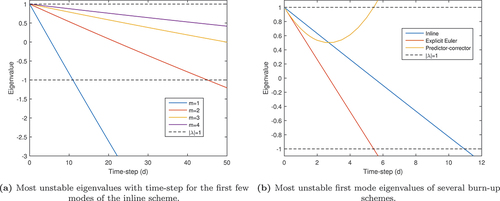
First, the stability eigenvalues of the first few spurious modes are shown for the inline depletion scheme in Fig. 1a, calculated by extracting eigenvalues from Eq. (57)(57a) ${\mathbf{G}}_{\omega }^{(c+1)}={\mathbf{B}}_0^{\mathrm{L}\mathrm{I}}+{\mathrm{\partial }}_{{\varphi }_n}{\mathbf{B}}^{\mathrm{L}\mathrm{I}}{N}_0{\mathrm{\Phi }}_{\omega }^{\mathrm{T}}+{\mathrm{\partial }}_{{\varphi }_{n+1}}{\mathbf{B}}^{\mathrm{L}\mathrm{I}}{N}_0{H}_{\omega }^{(c+1)}$(57a) . Recall that the allowable frequencies are given by $\omega =\frac{m\pi }{L}\mathrm{\forall }m\in \mathbb{Z}$, such that the lowest spurious frequency that can appear is given by $m=1$. It should be highlighted that there are two eigenvalues per mode (given the stability matrix is 2 × 2), but only the most unstable is shown; the other is persistently about 1 for all frequencies, but slowly decreases with increasing time-step length. Notably, the scheme is not unconditionally stable; as is the case for most other burnup schemes, the first mode is the most unstable. That said, the inline scheme is substantially more stable than both the explicit Euler and predictor-corrector schemes applied to the same problem, as seen in Fig. 1b (with their stability matrices coming from Refs. 18 and 19, respectively).

Fig. 1. Stability properties of the inline scheme applied to the two-nuclide system.

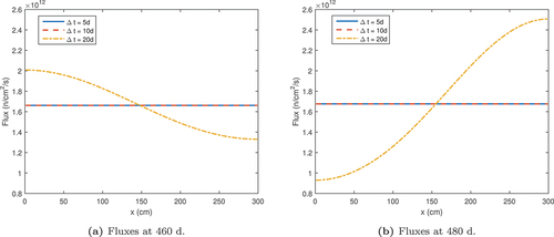
A numerical demonstration of the inline scheme’s stability is shown in Fig. 2, with an oscillating instability growing when the stable time-step length of about 11 days is exceeded.

Fig. 2. Flux solutions produced by the inline scheme at subsequent time points.

IV.B. Eight-Nuclide System

The eight-nuclide system has cross sections (in barns):

${\sigma }_{\mathrm{a}}=\left[\begin{array}{c}31.4\\ 0.835\\ 0\\ 86.5\\ 50\\ 0\\ 128000\\ 0\end{array}\right],{\sigma }_{\mathrm{f}}=\left[\begin{array}{c}31.4\\ 0.005\\ 0\\ 86.5\\ 0\\ 0\\ 0\\ 0\end{array}\right],{\sigma }_{\mathrm{s}}=\left[\begin{array}{c}0\\ 0\\ 0\\ 0\\ 0\\ 0\\ 0\\ 13.5\end{array}\right].$

The ordering of these nuclides is the same as listed at the beginning of Sec. V. The three fissile isotopes are presumed to have identical fission yields for product nuclides, with 90% of fissions producing the generic product, 5% producing iodine, and 1% producing xenon. Hence (in barns),

$\mathbf{\Sigma }=\left[\begin{array}{cccccccc}-31.4& 0& 0& 0& 0& 0& 0& 0\\ 0& -0.835& 0& 0& 0& 0& 0& 0\\ 0& 8.3& 0& 0& 0& 0& 0& 0\\ 0& 0& 0& -86.5& 0& 0& 0& 0\\ 28.26& 0.0045& 0& 77.85& -50& 0& 0& 0\\ 1.57& 0.00025& 0& 4.325& 0& 0& 0& 0\\ 0.314& 0.0005& 0& 4.325& 0& 0& -128000& 0\\ 0& 0& 0& 0& 0& 0& 0& 0\end{array}\right].$

Only three of the nuclides undergo decay—neptunium, iodine, and xenon—with their standard half-lives used here. Hence (in h^–1),

$\mathbf{\Lambda }=ln2\left[\begin{array}{cccccccc}0& 0& 0& 0& 0& 0& 0& 0\\ 0& 0& 0& 0& 0& 0& 0& 0\\ 0& 0& -1/57.6& 0& 0& 0& 0& 0\\ 0& 0& 1/57.6& 0& 0& 0& 0& 0\\ 0& 0& 0& 0& 0& 0& 0& 0\\ 0& 0& 0& 0& 0& -1/7& 0& 0\\ 0& 0& 0& 0& 0& 1/7& -1/9.1& 0\\ 0& 0& 0& 0& 0& 0& 0& 0\end{array}\right].$

The initial nuclide density for the system corresponds to a fresh UO₂ pin. This is (in atom/b/cm)

$N_0=\left[\begin{array}{c}0.000394\\ 0.007389\\ 0\\ 0\\ 0\\ 0\\ 0\\ 0.31296\end{array}\right].$

Other quantities are mostly identical to the two-nuclide case: $\nu$ is 2.3 across all fissile nuclides, $\kappa$ is 200 MeV, and the problem is 3 m long. The power per unit area differs, in order to ensure a pressurized water reactor (PWR) power density of 104 W/cm³; hence, the power per unit area $P$ is $104L$ W/cm².

As there are eight nuclides, there will be eight eigenvalues governing the growth of each spurious mode. Hence, for simplicity of presentation, only the spectral radius (the maximum absolute eigenvalue) of a given mode will be shown. Furthermore, as discussed in Ref. 41, due to the initial xenon transient to which PWR-like problems are subjected, stability estimates evolve rapidly and substantially from the estimates given by fresh fuel without xenon and iodine. Therefore, the value of $N_0$ used to estimate stability uses the saturated values of xenon and iodine corresponding to xenon equilibrium; these are $3.5641\times {10}^{-9}$ and $5.8998\times {10}^{-9}$ atoms/b/cm, respectively.

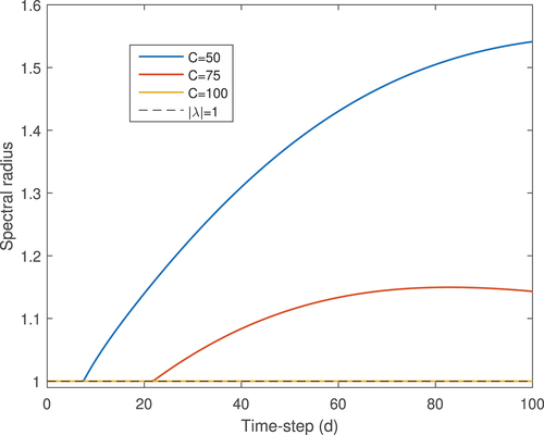
In this eight-nuclide system, as opposed to the two-nuclide system, the number of cycles/source iterations has a significant effect on stability. This is shown (before batching and relaxation) in Fig. 3. These results are relatively optimistic. For a semirealistic system of nuclides, with sufficient iterations, the inline scheme can be unconditionally stable. It is worth emphasizing that realistic problems of similar dimensions often require ~100 cycles to converge the fission source, at least when source convergence acceleration is not applied.

Fig. 3. Spectral radius of the inline scheme for various source iteration settings applied to the eight-nuclide system.

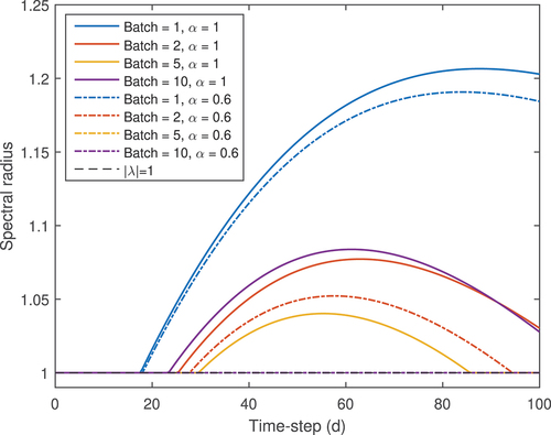
The stability of the system can be further improved by accumulating fluxes/reaction rates over several cycles and relaxing the nuclide density update, albeit there is an apparently optimal choice of batch size. This is shown in Fig. 4. Both the relaxed 5-batch and 10-batch stability estimates are co-linear and stable below one. The eigenvalues were extracted from Eq. (71)$\begin{array}{rl}& {\mathbf{G}}_{\omega }^{(l+1)}=\alpha \left({\mathbf{B}}_0^{\mathrm{L}\mathrm{I}}+{\mathrm{\partial }}_{{\varphi }_n}{\mathbf{B}}^{\mathrm{L}\mathrm{I}}{N}_0{\mathrm{\Phi }}_{\omega }^{\mathrm{T}}\right)\\ & +(1-\alpha ){\mathbf{G}}_{\omega }^{(l)}+\alpha {\mathrm{\partial }}_{{\varphi }_{n+1}}{\mathbf{B}}^{\mathrm{L}\mathrm{I}}{N}_0\\ & \frac{1}{J}\left[\sum _{j=0}^{J-1}{\rho }_{\omega }^j{H}_{\omega }^{(l)}+(1-{\delta }_{J-1}){\varphi }_0\right.\\ & \left.\sum _{j=1}^{J-1}\sum _{i=1}^j{\rho }_{\omega }^i\left(\frac{\nu {\sigma }_{\mathrm{f}}^{\mathrm{T}}}{\nu {\mathrm{\Sigma }}_{\mathrm{f},0}}-\frac{{\sigma }_{\mathrm{a}}^{\mathrm{T}}}{{\mathrm{\Sigma }}_{\mathrm{a},0}}\right){\mathbf{G}}_{\omega }^{(l)}\right].(71)\end{array}$. From this, one can see that choosing the batch size and relaxation factor well can result in an apparently unconditionally stable burnup scheme. One possible explanation for the apparently optimal batch size is the tradeoff between increasing the number of accumulation batches (which might approximately correspond to a relaxation) and performing additional corrector updates, which can better converge the nuclide densities; as the batch size increases, fewer corrector updates are performed for a fixed number of inactive/corrector cycles.

Fig. 4. Spectral radius of the inline scheme for various batch sizes and relaxation factors over 70 cycles applied to the eight-nuclide system.

Unfortunately, however, these stability results are overly optimistic. In spite of estimating stability with saturated xenon and iodine, the stability properties of each of the inline schemes evolves substantially with time. This behavior was originally highlighted in Ref. 41 for more traditional burnup schemes, although the changes in stability properties shown there were quite mild following some initial burnup. The evolution of the 70-cycle scheme with a batch size of five and a relaxation factor of 0.6 is shown in Fig. 5. This was generated by burning a one-region problem forward and using the resulting nuclide density to evaluate stability at different levels of burnup. In this figure, burnup is given in units of fissions per initial fissile atom (FIFA). Fortunately, performing the same exercise when applying 100 cycles with a batch size of five and a relaxation factor of 0.6 is apparently unconditionally stable (at least up to the same level of burnup). The relative stability of these two different settings is shown in Fig. 6. Perhaps reassuringly, the instability that emerges with 70 cycles takes a (nearly unphysically) long time to develop and even then its relative magnitude is quite small.

Fig. 5. Spectral radius of the inline scheme for different degrees of burnup when using 70 cycles, 5 cycles per batch, and a relaxation factor of 0.6.

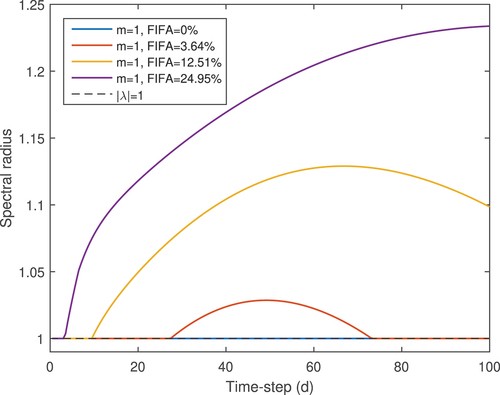
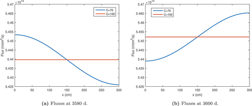
Fig. 6. Flux solutions produced by the inline scheme at subsequent time points for different numbers of cycles when applying a batch size of five and a relaxation factor of 0.6.

V. CONCLUSIONS

A new algorithm for burnup calculations was proposed in the style of methods applied to coupling neutronics with thermal hydraulics and xenon equilibrium. The stability properties of several variants of the algorithm were analyzed, and theory compared favorably with numerical results. Therefore, the algorithm appears to be an efficient means of stabilizing depletion, as well perhaps, as an efficient means of converging depletion alongside several other elements of reactor physics.

Work is currently under way to implement this proposed depletion algorithm in both Serpent²⁸ and SCONE (Ref. 43). This will allow for a fairer appraisal of the algorithm’s computational benefits in a high-fidelity Monte Carlo code, as well as how it performs when subjected to stochastic phenomena. Importantly, this will also allow the accuracy and efficiency of the algorithm to be examined when varying the statistics applied to obtaining a transport solution, i.e., subject to variations in the particle population per cycle. Furthermore, this will allow investigation of more complex chains of nuclides (such as the full chain resulting from ENDF or the CASL chain, as considered in Ref. 30) and their effects on stability. In the present paper, xenon and generic, absorbing fission products were examined under the presumption that they are responsible for much of the stability challenge. However, it may well be the case that prominent isotopes like samarium and gadolinium (which were not considered) may also pose unique challenges to the algorithm and stability.

Future work will consider how the presently proposed depletion algorithm interacts with the inline treatment of other physics, such as thermal hydraulics and xenon equilibrium; similar investigations were previously performed by Gill⁴ with promising results. In large, finely divided reactor problems, it is possible that repeated depletion calculations per time point may become comparable to or exceed the cost of the neutron transport calculations.²⁹ This might be partially circumvented either by using a smaller depletion system (at least during the inline portion of the algorithm),^29,30 or potentially through the use of a faster, reduced-order Bateman solver.⁴⁴ Finally, it should also be straightforward to extend the work to include higher-order burnup algorithms, e.g., with substepping, linear extrapolation, and quadratic interpolation.¹²

Disclosure Statement

No potential conflict of interest was reported by the authors.

Data Availability Statement

To the best of the authors’ knowledge, this paper and references herein contain all the data needed to reproduce and validate the results presented.

References

- D. P. GRIESHEIMER, “In-line Xenon Convergence Algorithm for Monte Carlo Reactor Calculations,” Proceedings of International Conference on Physics of Reactors (PHYSOR 2010), Pittsburgh, Pennsylvania (2010).
- D. F. GILL, D. P. GRIESHEIMER, and D. L. AUMILLER, “Numerical Methods in Coupled Monte Carlo and Thermal-Hydraulic Calculations,” Nucl. Sci. Eng., 185, 1, 194 (2017); https://doi.org/10.13182/NSE16-3.
- M. KREHER, B. FORGET, and K. SMITH, “Single-Batch Monte Carlo Multiphysics Coupling,” Proceedings of International Conference on Mathematics and Computational Methods Applied to Nuclear Science and Engineering, Portland, Oregon. (2019).
- D. GILL, “Inline Thermal and Xenon Feedback Iterations in Monte Carlo Reactor Calculations,” Proceedings of PHYSOR2020 – International Conference on Physics of Reactors: Transition to a Scalable Nuclear Future, Cambridge, UK (2020).
- B. KOCHUNAS, A. FITZGERALD, and E. LARSEN, “Fourier Analysis of Iteration Schemes for k-eigenvalue Transport Problems with Flux-Dependent Cross Sections,” J. Comput. Phys., 345, 294 (2017); https://doi.org/10.1016/j.jcp.2017.05.028.
- J. P. SENECAL and W. JI, “Approaches for Mitigating Over-Solving in Multiphysics Simulations,” Int. J. Numer. Methods Eng., 112, 6, 503 (2017); https://doi.org/10.1002/nme.5516.
- Q. SHEN, N. ADAMOWICZ, and B. KOCHUNAS, “Relationship Between Relaxation and Partial Convergence of Nonlinear Diffusion Acceleration for Problems with Feedback,” Proceedings of International Conference on Mathematics and Computational Methods Applied to Nuclear Science and Engineering, Portland, Oregon. (2019).
- Q. SHEN et al., “X-CMFD: A Robust Iteration Scheme for CMFD-based Acceleration of Neutron Transport Problems with Nonlinear Feedback,” Proceedings of International Conference on Mathematics and Computational Methods Applied to Nuclear Science and Engineering, Portland, Oregon. (2019).
- Q. SHEN and B. KOCHUNAS, “A Robust Relaxation-Free Multiphysics Iteration Scheme for CMFD-Accelerated Neutron Transport k-Eigenvalue Calculations—I: Theory,” Nucl. Sci. Eng., 195, 1176 (2021); https://doi.org/10.1080/00295639.2021.1906585.
- Q. SHEN, S. CHOI, and B. KOCHUNAS, “A Robust Relaxation-Free Multiphysics Iteration Scheme for CMFD—Accelerated Neutron Transport k-Eigenvalue calculation—II: Numerical Results,” Nucl. Sci. Eng., 195, 1202 (2021); https://doi.org/10.1080/00295639.2021.1906586.
- A. ISOTALO and P. AARNIO, “Higher Order Methods for Burnup Calculations with Bateman Solutions,” Ann. Nucl. Energy, 38, 1987 (2011); https://doi.org/10.1016/j.anucene.2011.04.022.
- A. ISOTALO and P. AARNIO, “Substep Methods for Burnup Calculations with Bateman Solutions,” Ann. Nucl. Energy, 38, 11, 2509 (2011); https://doi.org/10.1016/j.anucene.2011.07.012.
- A. ISOTALO and V. SAHLBERG, “Comparison of Neutronics-Depletion Coupling Schemes for Burnup Calculations,” Nucl. Sci. Eng., 179, 4, 434 (2015); https://doi.org/10.13182/NSE14-35.
- C. JOSEY, B. FORGET, and K. SMITH, “High Order Methods for the Integration of the Bateman Equations and Other Problems of the Form of Y´ = F(y, T) Y,” J. Comput. Phys., 350, 296 (2017); https://doi.org/10.1016/j.jcp.2017.08.025.
- J. DUFEK and J. E. HOOGENBOOM, “Numerical Stability of Existing Monte Carlo Burnup Codes in Cycle Calculations of Critical Reactors,” Nucl. Sci. Eng., 162, 3, 307 (2009); https://doi.org/10.13182/NSE08-69TN.
- J. DUFEK et al., “Numerical Stability of the Predictor-Corrector Method in Monte Carlo Burnup Calculations of Critical Reactors,” Ann. Nucl. Energy, 56, 34 (2013); https://doi.org/10.1016/j.anucene.2013.01.018.
- D. KOTLYAR and E. SHWAGERAUS, “On the Use of Predictor-Corrector Method for Coupled Monte Carlo Burnup Codes,” Ann. Nucl. Energy, 58, 228 (2013); https://doi.org/10.1016/j.anucene.2013.03.034.
- J. D. DENSMORE, D. F. GILL, and D. P. GRIESHEIMER, “Stability Analysis of Burnup Calculations,” Trans. Am. Nucl. Soc., 109, 695 (2013); https://doi.org/10.1007/s10967-012-2210-3.2.
- P. COSGROVE, E. SHWAGERAUS, and G. T. PARKS, “Stability Analysis of Predictor-Corrector Schemes for Coupling Neutronics and Depletion,” Ann. Nucl. Energy, 149, 107781 ( Dec. 2020); https://doi.org/10.1016/j.anucene.2020.107781.
- A. E. ISOTALO, J. LEPPÄNEN, and J. DUFEK, “Preventing Xenon Oscillations in Monte Carlo Burnup Calculations by Enforcing Equilibrium Xenon Distribution,” Ann. Nucl. Energy, 60, 78 (2013); https://doi.org/10.1016/j.anucene.2013.04.031.
- J. DUFEK, D. KOTLYAR, and E. SHWAGERAUS, “The Stochastic Implicit Euler Method: A Stable Coupling Scheme for Monte Carlo Burnup Calculations,” Ann. Nucl. Energy, 60, 295 (2013); https://doi.org/10.1016/j.anucene.2013.05.015.
- D. KOTLYAR and E. SHWAGERAUS, “Numerically Stable Monte Carlo-Burnup-Thermal Hydraulic Coupling Schemes,” Ann. Nucl. Energy, 63, 371 (2014); https://doi.org/10.1016/j.anucene.2013.08.016.
- D. KOTLYAR and E. SHWAGERAUS, “Stochastic Semi-Implicit Substep Method for Coupled Depletion Monte-Carlo Codes,” Ann. Nucl. Energy, 92, 52 (2016); https://doi.org/10.1016/j.anucene.2016.01.022.
- C. JOSEY, “Development and Analysis of High Order Neutron Transport-Depletion Coupling Algorithms,” Massachusetts Institute of Technology, Department of Nuclear Science and Engineering, PhD Thesis (2017).
- V. VALTAVIRTA and J. LEPPÄNEN, “New Stochastic Substep Based Burnup Scheme for Serpent,” PHYSOR 2018: Reactor Physics paving the way towards more efficient systems, Cancun, Mexico, 2, (2018).
- P. COSGROVE, E. SHWAGERAUS, and G. T. PARKS, “A Simple Implicit Coupling Scheme for Monte Carlo Neutronics and Isotopic Depletion,” Ann. Nucl. Energy, 141, 107374 (June 2020); https://doi.org/10.1016/j.anucene.2020.107374.
- P. COSGROVE, “Numerical Stability of Monte Carlo Neutron Transport and Isotopic Depletion for Nuclear Reactor Analysis,” University of Cambridge, PhD Thesis (2020).
- J. LEPPÄNEN et al., “The Serpent Monte Carlo Code: Status, Development and Applications in 2013,” Ann. Nucl. Energy, 82, 142 (2015); https://doi.org/10.1016/j.anucene.2014.08.024.
- D. P. GRIESHEIMER, D. C. CARPENTER, and M. H. STEDRY, “Practical Techniques for Large-Scale Monte Carlo Reactor Depletion Calculatons,” Prog. Nucl. Energy, 101, 409 (2017); https://doi.org/10.1016/j.pnucene.2017.05.018.
- P. K. ROMANO et al., “Depletion Capabilities in the OpenMC Monte Carlo Particle Transport Code,” Ann. Nucl. Energy, 152, 107989 (Mar. 2021); https://doi.org/10.1016/j.anucene.2020.107989.
- G. BELL and S. GLASSTONE, “Nuclear Reactor Theory,” US Atomic Energy Commission, Washington, DC (1970).
- C. MOLER and C. V. LOAN, “Nineteen Dubious Ways to Compute the Exponential of a Matrix, Twenty-Five Years Later,” SIAM Rev., 45, 1, 3 (2003); https://doi.org/10.1137/S00361445024180.
- M. PUSA and J. LEPPÄNEN, “Computing the Matrix Exponential in Burnup Calculations,” Nucl. Sci. Eng., 164, 2, 140 (2010); https://doi.org/10.13182/NSE09-14.
- M. PUSA, “Rational Approximations to the Matrix Exponential in Burnup Calculations,” Nucl. Sci. Eng., 169, 2, 155 (2011); https://doi.org/10.13182/NSE10-81.
- J. C. SUBLET et al., “FISPACT-II: An Advanced Simulation System for Activation, Transmutation and Material Modelling,” Nucl. Data Sheets, 139, 77 (2017); https://doi.org/10.1016/j.nds.2017.01.002.
- M. ELLIS et al., “Spatially Continuous Depletion Algorithm for Monte Carlo Simulations,” Trans. Am. Nucl. Soc., 115, 1.
- D. GRIESHEIMER et al., “MC21 V.6.0—A Continuous-Energy Monte Carlo Particle Transport Code with Integrated Reactor Feedback Capabilities,” Ann. Nucl. Energy, 82, 29 (2015); https://doi.org/10.1016/j.anucene.2014.08.020.
- H. ROBBINS and S. MONRO, “A Stochastic Approximation Method,” Ann. Math. Statist., 22, 3, 400 (1951); https://doi.org/10.1214/aoms/1177729586.
- N. ADAMOWICZ and P. COSGROVE, “Recent Advances in the Stability Analysis of Burn-Up Calculations,” Proc. M&C 2021, Raleigh, North Carolina (2021).
- P. COSGROVE and N. ADAMOWICZ, “Stability Analysis of Spatial Discretisation in Burn-Up Calculations,” Proc. M&C 2021, Raleigh, North Carolina (2021).
- P. COSGROVE and E. SHWAGERAUS, “Stability Analysis of Higher-Order Neutronics-Depletion Coupling Schemes and Bateman Operators,” J. Comput. Phys., 448, 110702 ( Jan. 2022); https://doi.org/10.1016/j.jcp.2021.110702.
- J. LIEBEROTH, “A Monte Carlo Technique to Solve the Static Eigenvalue Problem of the Boltzmann Transport Equation,” Nukleonik, 11, 213 (1968).
- M. A. KOWALSKI et al., “Scone: A Student-Oriented Modifiable Monte Carlo Particle Transport Framework,” J. Nucl. Eng., 2, 1, 57 (2021); https://doi.org/10.3390/jne2010006.
- C. CASTAGNA et al., “Development of a Reduced Order Model for Fuel Burnup Analysis,” Energies, 13, 4, 890 (2020); https://doi.org/10.3390/en13040890.