
 ?Mathematical formulae have been encoded as MathML and are displayed in this HTML version using MathJax in order to improve their display. Uncheck the box to turn MathJax off. This feature requires Javascript. Click on a formula to zoom.
Abstract
A novel source convergence acceleration method for Monte Carlo eigenvalue calculations is proposed in this paper. The method consists of simulating the bulk of the inactive cycles with online-generated multigroup cross sections. Then the active cycles are simulated with continuous-energy cross sections to preserve full fidelity. The method was implemented in the Monte Carlo code SCONE and tested on several three-dimensional full-length assembly models. In some cases, the same multigroup cross sections were used for several spatially separated materials in order to limit statistical uncertainties. The method was shown to accelerate calculations by a factor of 2.5 to 5 at the cost of a slightly increased standard deviation in the flux distribution estimated across several independent simulations. The memory usage due to storing multigroup cross sections does not seem to be prohibitive for practical applications.
I. INTRODUCTION
Monte Carlo is one of the most popular neutron transport methods. Its most prominent features are being high fidelity but relatively computationally expensive. Historically, its main use was to perform reference calculations for code-to-code benchmarks, although with more available computing power it is seeing increasingly routine use across industry and academia for reactor analysis and design. In order to extend the range of problems to which it can conveniently be applied, several methods to speed up Monte Carlo transport simulations are being investigated.
A subclass of acceleration strategies is source convergence acceleration. Monte Carlo criticality calculations use a convergence method analogous to the power iteration method used by deterministic methods.Citation1 Starting from a guess neutron fission source and fundamental eigenvalue, a transport calculation is performed in order to obtain the next step’s fission source and eigenvalue. The process is repeated until convergence is reached by some chosen measure. Since the first steps, called inactive cycles in Monte Carlo, produce biased estimates due to the unconverged fission source, they are normally excluded from the final results. The cycles that actually contribute to the collection of statistics to calculate the final results are called active.
In many criticality safety models, e.g., metallic spheres, the dominance ratio is low and convergence to the fundamental fission source is achieved very rapidly. As such, most of the computational time is spent on accumulating statistics during the active cycles. However, in certain cases the inactive cycles can take the largest fraction of the total computational time. In problems with a high dominance ratio, such as full-length three-dimensional (3-D) reactor models, it might take several hundreds of cycles before the source converges as measured by the Shannon entropy.Citation2,Citation3 As an example, a full-core pressurized water reactor (PWR) can have a dominance ratio larger than 0.99; the 3-D BEAVRS reactor’s dominance ratio is estimated to be 0.996 (CitationRef. 3). At the same time, the same models might be subject to issues such as clustering and correlation effects, which are partially controlled by increasing the neutron population.Citation4 If the number of neutrons per cycle is large enough, the number of active cycles needed to achieve acceptable statistical uncertainties can be relatively low. However, the number of iterations needed for the problem to converge is independent of the neutron population. Therefore, it might be the case that the number of inactive cycles needed largely exceeds the number of active cycles, thus becoming extremely computationally expensive when large populations are necessary.
To obviate this problem, several methods to accelerate source convergence have been devised. Some of these achieve convergence acceleration by reducing the number of full-fidelity Monte Carlo inactive cycles needed. This is possible if a good fission source guess, produced by a cheaper transport or diffusion solver, is provided. Typically, the cheaper solver is a deterministic method. This is the case, for example, of response matrix accelerationCitation5 developed within the Monte Carlo code Serpent.Citation6 In this method, a slightly modified Monte Carlo inactive cycle is used to generate coefficients for a deterministic response matrix solver that can provide a good fission source guess. The method was tested on a 3-D full-reactor model and accelerated source convergence considerably. The main limitation is that, in order for the deterministic solver to converge avoiding instabilities, good coarse and fine spatial meshes must be provided by the user. However, choosing the optimal mesh is nontrivial and might require a trial and error approach.
Another method is coarse mesh finite difference (CMFD) acceleration. CMFD is commonly used to accelerate deterministic methods, while it was first applied to Monte Carlo transport by CitationRef. 7. Given a coarse mesh, the coefficients for a multigroup (MG) diffusion calculation can be obtained during one or several Monte Carlo inactive cycles. By solving a diffusion equation that is forced to be consistent with the transport solution via a correction factor, the weights of the Monte Carlo source neutrons for the next cycle can be modified to match the diffusion solution. This is repeated until convergence is reached. CMFD has been shown to accelerate convergence substantially, reducing the inactive cycles required by a factor of at least 3 in large reactor problems.Citation3 One of the difficulties of CMFD is that it might be affected by numerical instabilities.Citation8 This can be avoided by choosing the coarse mesh parameters wisely. A similar, but more uniquely Monte Carlo approach, is fission matrix acceleration.Citation9 This method also modifies particle weights between inactive cycles, but it is informed by estimating the discretized Green’s function for fission neutrons born in different regions of the problem at hand.
A different category of convergence acceleration strategies aims at making the inactive cycles less expensive, rather than reducing the number of inactive cycles needed. An example of such methods is particle ramping,Citation10 where the neutron population is initially low and it is gradually increased as the inactive cycles proceed. While this method can surely accelerate the simulation, it may be prone to negative correlation effects due to the whole neutron population originating from a small number of families.
This work proposes a novel source convergence acceleration method for reactor calculations that falls under the latter category. Its goal is to speed up the inactive cycles by using MG data instead of continuous-energy (CE) data. Due to reduced memory access, the use of MG data is known to substantially accelerate Monte Carlo neutron transport.Citation11 This method was introduced in CitationRef. 12, and it is expanded here. The rest of this paper is structured as follows. The methodology is described in Sec. II, the numerical investigations carried out and the results found are presented in Sec. III, and the conclusions are drawn in Sec. IV.
II. METHODOLOGY
One of the computational bottlenecks of Monte Carlo particle transport codes is appreciated to be the retrieval of CE cross sections.Citation13 CE cross sections may lie on energy grids, including up to 1 million points, which makes the grid search process expensive. Additionally, this large amount of data must be stored in a deep layer of the computer memory. Accessing these data in the memory is an expensive operation that must be performed several times per each neutron track during a transport simulation. However, this bottleneck can be alleviated by using MG nuclear data. MG nuclear data normally lies on much coarser energy grids that can be kept closer in memory, offering a large speedup at the cost of lower fidelity. MG cross sections are materialwise rather than nuclidewise and treat scattering via scattering matrices rather than scattering laws. Data are more compact and faster to process: acceleration factors of 5/6 can be expected when transitioning from CE to MG.
The methodology applied in this paper is an extension of CitationRef. 12. The approach aims at accelerating fission source convergence by simulating most of the inactive cycles with MG cross sections. The same group structure was used per each set of cross sections. This algorithm is implemented in the Monte Carlo code SCONE (CitationRef. 14). SCONE has the unique feature of allowing the use of different cross-section representations simultaneously or in the same calculation. In CitationRef. 12, the MG cross sections were pregenerated via a Serpent run and fed into SCONE for simulating the bulk of the inactive cycles. Only a small number of final inactive cycles was simulated with CE cross sections in order to ensure convergence to the correct fission source. The transition from one cross-section type to the other was possible thanks to the implementation of a routine that can switch from MG to CE nuclear data from one cycle to the other. This operation requires resampling the energy of the particles contained in the neutron bank for the following cycle from the correct CE fission spectrum. This was done by sampling one of the fissile nuclides in the material each particle is in based on their fission cross section at 1 eV; then a neutron energy from the thermal fission spectrum of the nuclide selected is sampled. The energy used to sample the fissioning nuclide is arbitrary and could be changed. However, in this case, given that the method was tested on light water reactors (LWRs), 1 eV seemed an appropriate value. Although the choice of a fixed energy introduces an approximation, the error added is expected to be negligible and to disappear after a single or very few CE cycles. Afterward, the active cycles are simulated with CE cross sections to obtain full-fidelity results.
In this work, the main difference with respect to CitationRef. 12 is that MG cross sections are generated online during the first few inactive cycles. This is possible because the fission source does not need to be converged for efficient cross-section generation. This feature allows for preparing and performing a MG calculation in only one step, removing the need for the preliminary Serpent calculation used in the preceding work. A similar approach is applied, for example, when using CMFD acceleration.Citation3 To summarize, the new calculation routine consists of the following steps:
Running some CE inactive cycles for MG cross-section generation.
Initializing the MG materials with the calculated cross sections.
Resampling the energy of the fission source neutrons from a MG spectrum.
Running a certain number of MG cycles.
Resampling the energy of the fission source neutrons from a CE spectrum.
Running the remainder of the inactive cycles and all of the active cycles with CE data.
To allow this, new features had to be developed in SCONE. The capability to generate MG cross sections was introduced, as well as a subroutine to transition from CE to MG nuclear data at the end of a cycle. Other than the usual population parameters, such as number of active and inactive cycles and neutron population per cycle, other parameters can now be varied by the user. These are the number of cycles dedicated to cross-section generation and the number of final CE inactive cycles. The next section describes the MG cross-section generation procedure implemented in SCONE.
II.A. Cross-Section Generation
The MG cross sections need to account for energy and spatial self-shielding effects. One of the advantages of generating them with Monte Carlo is that self-shielding is taken into account automatically and approximate treatments like equivalence theory are not necessary. In SCONE, the cross-section generation methodology was inspired by CitationRefs. 15 and Citation16. A new tally type was implemented to introduce the cross-section generation capability. Given a user-defined energy group structure, the MG cross section in group for a generic reaction
,
, is calculated as described by EquationEq. (1)
(1)
(1) per each material or group of materials:
where and
are the CE cross section and scalar neutron flux, respectively. The average number of neutrons per fission
is calculated as shown in EquationEq. (2)
(2)
(2) :
The scattering matrices are normally calculated from the scattering double-differential cross sections , as shown in EquationEqs. (3)
(3)
(3) and Equation(4)
(4)
(4) :
and
where is the l’th Legendre polynomial, and
is the corresponding scattering matrix. However, similarly to MCNP and Serpent, SCONE reads nuclear data from ACE files, which do not include such cross sections. An alternative method, proposed in CitationRef. 15, consists of calculating the probability of scattering from group
to
,
, with an analog estimator. This can then be used to estimate the scattering matrices as in EquationEqs. (5)
(5)
(5) and (Equation6
(6)
(6) ), which refer to Legendre polynomial orders 0 and 1, respectively:
and
where the average scattering angle cosine is also estimated with an analogue estimator.
For this work, only the and
scattering matrices were generated since SCONE cannot read higher anisotropy moments. However, the
scattering representation was assumed to be sufficient for the models simulated in this work, given they are LWR problems and as such do not present strong anisotropy. Alternatively, transport-corrected
scattering would also be suitable to treat higher anisotropy, provided the transport-corrected cross sections were appropriately generated. This approach would be preferable, since it would also reduce memory consumption.
An analogue estimator was used also for the MG fission neutron spectrum :
The cross sections generated by SCONE were compared to those produced by Serpent for the problems investigated, and they agree well within uncertainties.
III. NUMERICAL INVESTIGATIONS
The goal of this work is to demonstrate whether the proposed method can accelerate simulations while maintaining full fidelity. There are a few parameters that can be varied to achieve this: the number of cross-section generation cycles, the number of energy groups used, the number of unique MG material regions, and the number of final CE inactive cycles. It is desirable to minimize the number of CE inactive cycles used to obtain the maximum speedup possible. At the same time, however, one must ensure that full convergence is achieved to get unbiased scores during the active cycles. For this, using a finer group structure might be useful. Conveniently, the time taken by MG transport is basically unaffected by the group structure; this was seen in the current work varying the number of groups from 7 to 69. However, the finer the group structure, the larger the number of particles needed to produce reliable cross sections given the statistical fluctuations. The use of more groups would thus result in more initial CE cycles, but it might allow for reducing the number of final CE cycles. On the contrary, using a smaller group structure might allow for reducing the number of initial CE cycles. However, in some cases this can come at the cost of a disproportionately larger amount of final CE cycles. This is the case because few-group structures might not capture all the relevant spectral effects and can converge to a different fission source. Therefore, final CE inactive cycles are needed to correct the source distribution. However, correcting the fission source after wrong convergence might take a considerable number of CE cycles. This is especially the case in slow converging problems, i.e., problems with a high dominance ratio. Similar concerns apply for the number of unique material regions for which cross sections may be generated; one can more accurately capture spatial spectral variations by generating MG cross sections in many small regions, but this would also entail increased variance.
The parameters chosen clearly depend on the number of neutrons simulated per cycle. For instance, a larger neutron population would reduce the number of cross-section generation cycles needed, but increase the weight of the inactive cycles on the total computational time. On the other hand, the lower bound for the neutron population is determined by correlation effects, often present in high dominance ratio problems, such as large 3-D reactors. Following these considerations, the method proposed was tested on several models and a sensitivity study on all parameters was performed.
In order to test the proposed acceleration method, three 3-D light water assembly/minireactor models were simulated. These are a fresh-fuel PWR assembly, a CE version of the C5G7 benchmark model, and a PWR assembly with burnt fuel composition. Since SCONE does not support parallel calculations yet, a 3-D full-core model was deemed too computationally expensive to simulate for this paper. However, these models were chosen because they have different challenging features. The fresh PWR assembly contains heavy absorbers in the form of gadolinium-bearing pins; the C5G7 introduces a mixed-oxide (MOX) and uranium-oxide reflector interface with large spectral differences; and the burnt PWR assembly allowed for testing the method on a burnt problem, where each fuel pin has a different material composition.
For each model, different population parameters were used. Generally, a large number of inactive cycles was chosen to guarantee full convergence. For the BEAVRS benchmark, which has a relatively high dominance ratio, 200 inactive cycles were sufficient for convergence without any source convergence acceleration.Citation3 In order to be conservative, at least 300 inactive cycles were used for the models simulated in this paper. At the same time, a relatively large neutron population was necessary to limit high statistical fluctuations, as well as correlation effects.Citation17 For the same reasons, all results were averaged over eight independent runs. On particle numbers, it seems common in literature to use on the order of hundreds of millions of active neutron histories to simulate a full 3-D PWR core.Citation18,Citation19 As a consequence, 160 million total histories seem appropriate for a single or few 3-D PWR assemblies. The number of active cycles was chosen to be low, since it was previously demonstrated that lowering the number of neutrons per cycle (keeping the number of total neutron histories constant) is effective in reducing variance while using simulation time economically. This is due to intergenerational correlation; increasing the number of active cycles does not reduce the true standard deviation of estimates according to the ideal trend.Citation3,Citation20 The state of convergence was monitored through Shannon entropy,Citation2 as well as through the final axial and radial flux profiles. All simulations were run on a single Intel® Xeon® Gold 6130 2.10 GHz CPU core, without parallelization.
III.A. Full-Length Fresh Assembly
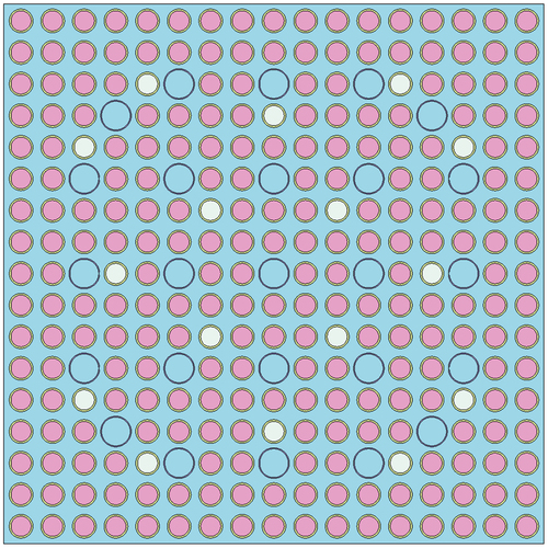
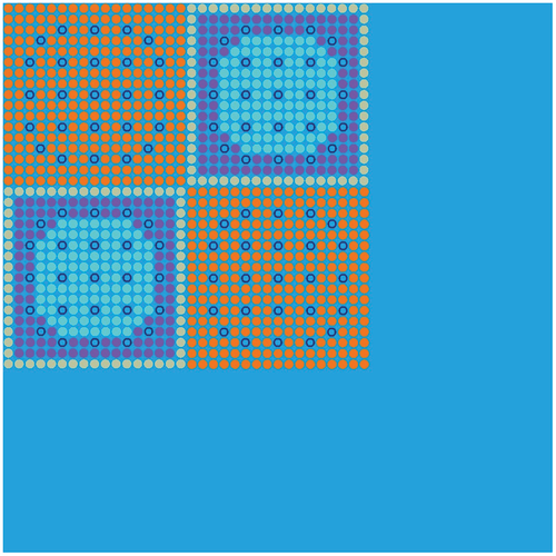
The first model tested is a 3.6-m-long PWR assembly with gadolinium pins and water-filled guide tubes. The fuel is 4.2% enriched UO2; gadolinium-bearing pins are made of 2.7% enriched UO2, with 6.6 mole % of Gd2O3, where gadolinium has a natural isotopic composition. The model radial configuration is shown in . Axially, a realistic water density profile was introduced by dividing the moderator material into 10 axial nodes. The density profile is reported in , where the density of node 10 corresponds to 0.75425 g/cm3. In order to capture axial spectral variations, the fissile materials also were split into 10 axial nodes for cross-section generation. Radially, in a given axial node, all UO2 pins have the same MG cross sections, as have the gadolinium-bearing pins. The boundary conditions applied are radially reflective and axially vacuum. For this model, 1 million particles per cycle, 400 inactive cycles, and 20 active cycles were simulated. While a large number of inactive cycles were utilized to ensure convergence, few active cycles were enough to get good statistical accuracy given the relatively high neutron population.
TABLE I Density Profile of Water Coolant Where Node 1 Corresponds to the Top of the Assembly
Fig. 1. Radial cross-section view of the PWR assembly geometry.
An identical model was simulated to test the method in CitationRef. 12, which is identical to the method presented in this paper with the exception that cross sections were precalculated by a Serpent run. In that work, the Shannon entropy was calculated axially over 20, 50, and 100 axial bins, as well as radially with a pin-by-pin discretization. The result was that, even though in some cases the final axial flux profile differed up to 4%, the Shannon entropies calculated with the different axial discretizations agreed perfectly. This implies that in these cases the MG calculation converged to a slightly incorrect fission source, biasing the final flux distribution, and this was not captured in the Shannon entropy measurement. When different population parameters were applied, the axial flux profile improved considerably, while the Shannon entropy did not change. Given these observations, in this work Shannon entropy is treated as an approximate convergence measure. Whether the MG-accelerated calculation converged properly, thus ensuring full-fidelity results, will be determined instead by comparing the final flux profiles.
Additionally, CitationRef. 12 showed that the pin-by-pin radial entropy converges within five inactive cycles for this model, and the pin-by-pin radial flux error was below or equal to 0.1% for all cases considered. This was the case also when the axial flux profile was not satisfactory. Following these considerations, radial entropy and flux measurements were not scored for this model.
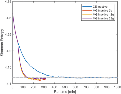
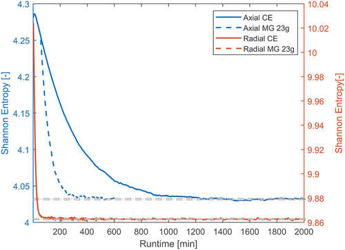
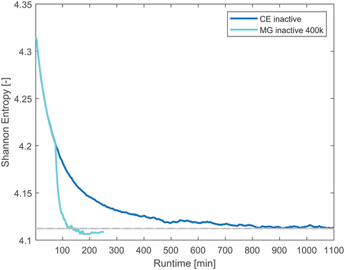
Some results for the PWR assembly are shown next. The results from CitationRef. 12 were used as a starting point to choose the simulation parameters. In that work, for the same model, seven groups with 25 final CE inactive cycles produced satisfactory results. When only 10 final CE cycles were used, the flux deviation reached up to 4%. Here, several group structures were used; these are the CASMO7 −12 and −23 energy grids optimized for LWRs. For this group structure comparison, all cases included 20 cross-section generation cycles and 20 final CE cycles. The Shannon entropy, calculated over 20 axial bins, is shown in . The entropy looks fully converged for all cases, and using a finer group structure seems to slightly improve the entropy value when compared with the CE reference. shows the Shannon entropy as a function of run time rather than cycle number. The solid and dashed gray lines in the plot represent, respectively, the mean and standard deviation of the converged CE entropy calculated over the final 100 cycles. The 23-group case entropy is within one standard deviation of the reference one, while this is not the case for the 7- and 12-group cases. Interestingly, the 7-group entropy seems to be substantially offset from the reference value until approximately cycle 380, where the calculation is switched back to CE and the entropy changes trend. Using a finer group structure does not impact the computational time noticeably. When simulating 400 inactive cycles, the MG inactive cycles took approximately 70% less time to conclude than the CE ones. However, all simulations converged after about 200 cycles; this corresponds to around 500 min for the full CE calculation and 160 min for the MG ones. Considering that the last 20 cycles of the MG case have to be simulated with CE rather than MG, the calculation would be around 200 min long. Therefore, the MG-accelerated cases converge approximately 2.5 times faster than the CE simulations.
Fig. 2. Axial Shannon entropy for different group structures in the PWR assembly.
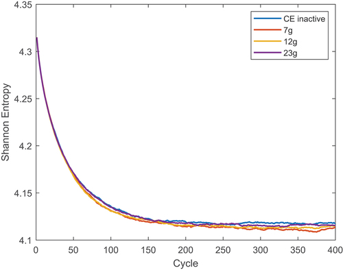
Fig. 3. Axial Shannon entropy for different group structures as a function of run time in the PWR assembly.
shows the cross-section uncertainties for the three different group structures when 20 CE generation cycles are used. An additional case with 23 groups and 10 CE generation cycles was also added. For all cases, a large difference between minimum and maximum uncertainty, reflected in large standard deviations, is present. A closer analysis showed that uncertainties are maximum on the materials at the top and bottom of the assemblies and minimum at the center. The large difference between minimum and maximum is thus justified by the presence of statistically insignificant regions. The average for capture and fission cross sections does not change heavily with the group structure. The expected trend on the average uncertainty, in particular, was not observed. This is probably due to correlation effects; it was previously observed by CitationRef. 3 that tallies do not follow the well-known
behavior in problems with a high dominance ratio because of the high coupling between successive generations of neutrons. Uncertainties are significant for the
matrix, whose dimensions are N
N. The average uncertainty in
increases considerably when increasing the group number from 12 to 23. Using 10 cycles instead of 20, however, does not produce a considerable difference. The results for the 23-group case with 10 cross-section generation cycles are shown later in this section.
TABLE II Cross-Section Uncertainties (in %) for the PWR Assembly Materials
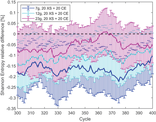
and show the relative difference between the entropies of the CE and MG cases when changing the number of generation cycles and number of energy groups, respectively. This is displayed for the last 100 inactive cycles. The error bars represent the standard deviation of the entropy between the eight independent runs. shows results for the 7-group structure. An attempt to maximize speedup was made by reducing the number of cross-section generation cycles. Even if the average value is not affected, decreasing the number of cross-section generation cycles increases the entropy variance. Although the large variance of the 5-cycle case suggests that the results are within the uncertainty of the reference, the reduced uncertainty of the 20-cycle case shows that using seven groups leads to a small systematic bias. In order to approach a more accurate source distribution, a finer group structure should be used, as shown in . Surprisingly, the standard deviations for all cases are similar. Evidently, the higher uncertainties in the scattering matrix of the 23-group case do not significantly affect the axial source profile. and are intended to show the effects of changing some simulation parameters on the mean and the variance of the Shannon entropy. Even if some trends can be seen by varying certain parameters, all results are within 0.2% of the reference Shannon entropy. Therefore, whether a substantial systematic bias was introduced or not by the MG cycles will be determined by examining the final flux distributions.
Fig. 4. Relative difference between MG and reference Shannon entropy when varying the number of cross-section generation cycles in the PWR assembly.
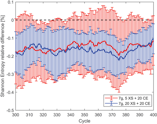
Fig. 5. Relative difference between MG and reference Shannon entropy when varying the group structure in the PWR assembly.
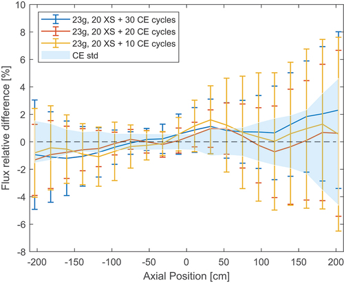
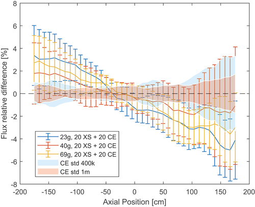
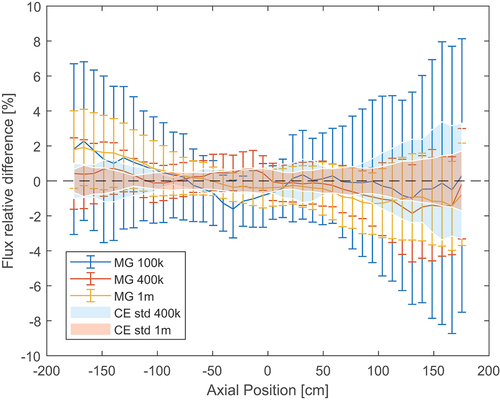
shows the axial flux profile calculated over 20 axial bins. The relative difference between different cases can be observed in and , where the error bars represent the uncertainty resulting from the standard deviation between independent runs. The blue area in the plots represents the standard deviation between independent CE runs as a term of comparison. In , the flux difference is compared for the three energy grids used. For all cases, both the mean errors and standard deviations increase at the extremities of the assembly, where the flux magnitude is lower and MG cross sections have extremely high uncertainties. Even if all fluxes agree within uncertainties, the average difference gets smaller when the number of groups is increased. In the 23-group case, the average difference is below 1.5%, and it is within the CE standard deviation band. At the same time, the uncertainties decrease when increasing the number of groups. Given that using 23 groups rather than 7 or 12 does not produce a significant time overhead, the CASMO23 group structure seems an appropriate choice for this model.
Fig. 6. Axial flux profile produced by different group structures in the PWR assembly.
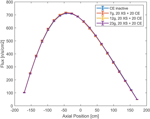
Fig. 7. Relative difference between MG and reference axial flux when varying the group structure in the PWR assembly.
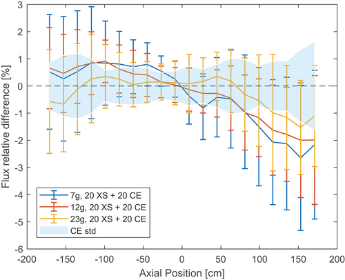
Fig. 8. Relative difference between MG and reference axial flux when using different cross-section generation and final CE cycle combinations in the PWR assembly.
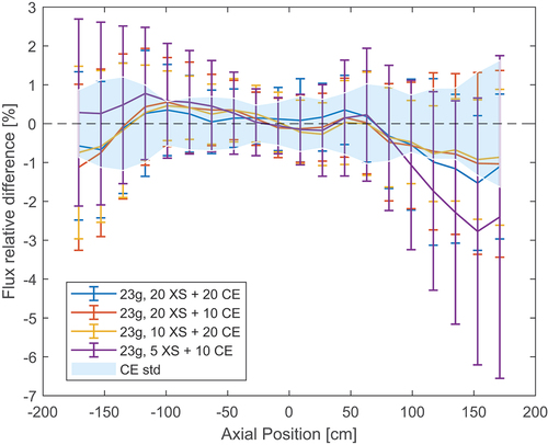
Reducing the total number of CE inactive cycles used in a simulation should improve the speedup. This can be achieved by reducing either the number of cross-section generation cycles or the number of final CE inactive cycles. In , several combinations were tried. The combinations 20 + 10 and 10 + 20 perform equally well; however, reducing the number of final CE inactive cycles increases the standard deviation between independent runs more than reducing the cross-section generation cycles. A more extreme case of 5 + 10 CE cycles was tried, but the error was outside of the CE standard deviation band and the standard deviation produced reached around 4%.
III.B. C5G7 Benchmark
The second model tested is a 3-D, 2 2 assembly configuration based on the C5G7 benchmark.Citation21 The model is made of two UO2 and two MOX assemblies surrounded by a thick water reflector. The MOX assemblies are made of pins with three different transuranic enrichments: 4.3%, 7.0%, and 8.7%. The fuel materials were homogenized with Zircaloy and aluminum claddings. The resulting pin radius is 0.54 cm. The fuel material densities are shown in . The radial configuration of the model can be seen in . Water guide tubes are present between the fuel pins. Axially, the assemblies are 385.56 cm long, and a 21.42-cm water reflector is added both at the top and at the bottom. The following boundary conditions are applied: radially, the boundaries adjacent to the assemblies were reflective while the others were vacuum. Axially, the top and bottom boundaries were vacuum. Additionally, a water axial profile, not present in the original benchmark, was introduced by splitting the water into 10 axial materials. The profile is identical to the one presented in , where the MOX materials are named after their respective transuranic enrichment. In this case, the density of node 10 is 1.0 g/cm3. All water materials also include 500 ppm of boron. In order to capture spectral variations, also all the fuel materials are split into 10 axial nodes for MG cross-section generation. All the materials in the benchmark use cross-section libraries at a temperature of 300 K. It is worth noting that in this case water is considerably denser than in the PWR assembly. The high water density decreases the neutron mean free path, making the reactor strongly decoupled. Since neutrons take a long time to travel from one end of the assembly to the other, convergence is extremely slow. In this case, 800 inactive cycles were run to ensure full convergence. The neutron population used was 1 million neutrons per cycle, with 20 active cycles.
TABLE III Atomic Densities of the C5G7 Fuel Materials*
Fig. 9. C5G7 benchmark radial configuration.
Shannon entropy was measured separately axially and radially, using 20 axial bins and a pin-by-pin subdivision, respectively. These results can be seen in and . In this case, the best group structure found in the previous case was used. This consists of the CASMO23 energy grid with 20 cross-section generation cycles; in order to ensure convergence in this extremely high dominance ratio problem, 30 final CE cycles were added. The radial entropy converges after less than 50 cycles. The fast radial convergence is due to the relatively small radial dimensions. On the other hand, the axial entropy takes approximately 500 cycles to converge. Applying the same reasoning as in the previous case, it can be concluded that the MG case converges approximately three times faster than the reference one.
Fig. 10. Axial and radial Shannon entropy for different group structures in C5G7.
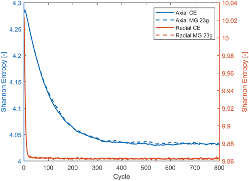
Fig. 11. Axial and radial Shannon entropy for different group structures as a function of run time in C5G7.
The cross-section uncertainties when 20 CE generation cycles are used are shown in . Like in the previous model, even if the average uncertainties observed are unacceptably large, the error is much smaller in statistically relevant regions. This is reflected in the results shown, which seem to imply that no bias is added as a result of the MG cycles.
TABLE IV Cross-Section Uncertainties (in %) for the C5G7 23-Group Case
shows the axial flux profile, while shows the relative error between the reference and the MG cases. The blue area in the plot represents the standard deviation between independent CE runs. In , an attempt to reduce the number of final CE cycles was made. All average errors are below 2% and within the standard deviation of the reference runs. However, even in the case with the largest number of CE cycles, the MG standard deviation is larger than the CE one. Decreasing the number of final CE inactive cycles increases the standard deviation even further. Potentially, reducing the number of cross section generation cycles could be attempted as well. However, this has not been included in this study.
Fig. 12. Axial flux profile produced by different group structures in C5G7.
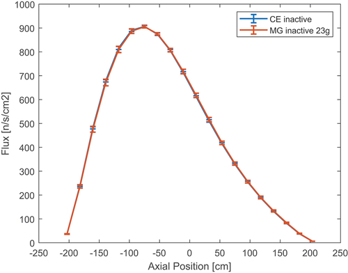
Fig. 13. Relative difference between MG and reference axial flux when using a different number of final CE cycles in C5G7.
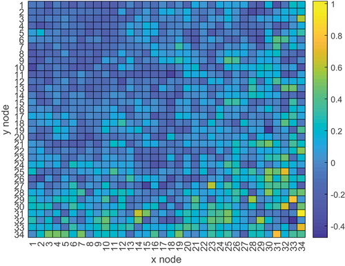
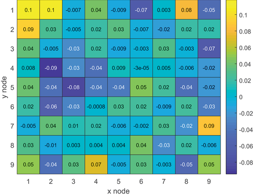
The reference radial flux is shown in , and the relative error between CE and MG is shown in . The MG case chosen was the one with 23 groups and the lowest number of CE cycles, i.e., 20 + 10. Once again, the radial features of the model can be reproduced more accurately than the axial ones. All pin errors are below 1%, and the average error is 0.15%.
Fig. 14. Reference radial flux profile in C5G7.
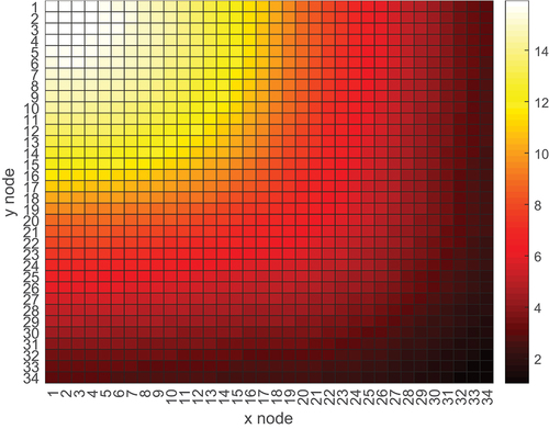
Fig. 15. Relative difference between 23-group MG (20 XS + 10 CE) and reference radial flux in C5G7.
III.C. Full-Length Burnt Assembly
The burnt PWR assembly consists of the same design as the first model, with the exception that the fuel has been burnt up to 10 MWd/kg. The gadolinium pins and the axial water density profile were included. The fuel composition was extracted from the results of a Serpent pin-by-pin depletion calculation on the fresh assembly, where all fissile materials were further split into 10 axial nodes. In building the SCONE model, the 1/8 symmetry of the geometry was exploited, so that the total number of materials to be defined could be reduced. The base portion of the assembly is shown in . This model resulted in a combination of 402 materials containing 201 nuclides overall.
Fig. 16. Portion of burnt PWR assembly adopted for 1/8 symmetry.
Initially, the same simulation strategy as for the other models was chosen. This includes generating a different set of cross sections per each material in the geometry. In this case, given the substantial computational cost of running a model with many nuclides, 400 000 neutrons per cycle were also used, along with 300 inactive cycles and 30 active cycles. The results produced are shown in . The blue and red bands in the plots represent the standard deviation between reference CE runs with, respectively, 400 000 and 1 million neutrons per cycle. Initially, the CASMO23 group structure, successful for the previous models, was used. However, this produced an error around 4% with a standard deviation also around 4%. Increasing the number of groups and adopting the CASMO40 group structure improved the results, while using the WIMS69 group structure produced an intermediate error. Increasing the number of final CE inactive cycles improved the results only slightly, thus they are not shown here.
Fig. 17. Relative difference between MG and reference axial flux when using different group structures in the burnt PWR assembly.
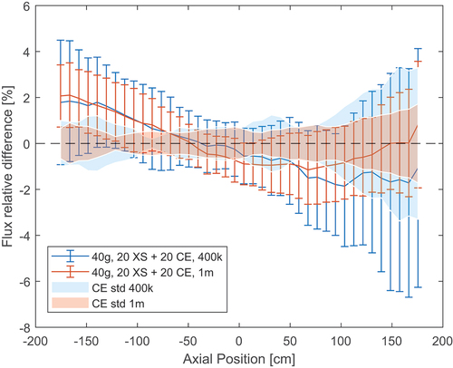
Given the large number of materials and nuclides present in this model, memory consumption might also become a concern. This is especially the case when relatively fine group structures are used, like the WIMS69 grid. Since this is the most memory-intensive model simulated in this paper, memory utilization was measured for this model only. The memory consumption was found to be 217 MB in the reference CE case, 254 MB when 23 groups were used, and 431 MB when 69 groups were used. The memory usage almost doubled when 69 group cross sections were generated due to the large scattering matrices, indicating that this method could easily become memory intensive in certain cases. However, the memory increase was more modest when only 23 groups were used. In order to try to reduce the correlation effects that originated from the lower neutron population used and were possibly responsible for the large errors, a population of 1 million neutrons per cycle was tried as well. The results are shown in . Increasing the neutron population improved the flux difference and reduced the standard deviation considerably. Even if the flux error is now consistently below 2%, it is still outside the CE standard deviation bands.
Fig. 18. Relative difference between MG and reference axial flux when using different neutron populations in the burnt PWR assembly.
The high error observed was found to be caused by the extremely high cross-section uncertainties presented in . Also in this case, 20 CE generation cycles were used. Contrary to the other cases, capture and fission cross-section uncertainties now differ more significantly. In particular, it is interesting to observe the minimum uncertainty values found. While this is around 1% for capture, it is larger than 10% for fission. While capture includes both water and fuel materials, fission only refers to the fuel. It is clear that water cross sections have reasonably low uncertainties, but this is not the case for the fuel. While in previous models there were 20 to 40 fuel materials, this case includes 390 fuel materials. Therefore, to compensate, at least 10 times more particles or cross-section generation cycles should be employed. Using 10 times more generation cycles, however, would basically take the entirety of the inactive cycles. Additionally, it was previously mentioned that tallies do not follow a behavior in high correlation models. Therefore, more than 10 times more cycles would probably be needed. While, for the same reason, there is no clear trend between the uncertainties relative to 23, 40, and 69 groups, the 7-group structure has obviously lower uncertainties. However, the 7-group structure was found to be unable to provide proper convergence for a PWR assembly model with gadolinium pins. Due to these obvious limitations, another approach was attempted.
TABLE V Cross-Section Uncertainties (in %) for the Burnt PWR Assembly Materials
III.C.1. Material Grouping
From the previous results, it was found that a burnt problem could not be simulated in the same manner as done so far. In order to assure sufficient statistics to generate reliable cross sections, almost the entirety of the inactive cycles would have to be simulated with CE, defeating the goal of the method. As a consequence, the same cross sections were used for similar materials during the MG cycles. A single set of cross sections was generated for all the gadolinium-free fuel materials in each axial slice and for the gadolinium pins. The other materials were treated identically as before. This approach aims to reduce the uncertainties in cross-section generation, and it fulfills the purpose of reducing memory consumption as well. When using 23 groups, in this case the memory usage amounts to 220 MB rather than the previous 254 MB, while the reference CE case occupies 217 MB.
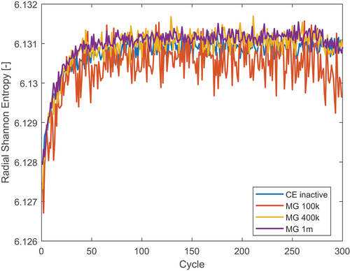
In the following calculation, parameters including 23 groups with 20 cross-section generation cycles and 20 final CE cycles, successful in modeling the fresh PWR assembly, were used. The new axial and radial Shannon entropies are presented in and . The axial entropy was calculated over 20 axial bins, and the radial one with a pin-by-pin discretization. Different neutron populations per cycle were used. The axial Shannon entropy converges in 250 cycles, while the radial entropy takes approximately 50 cycles. When only 100 000 particles are used, both entropies are extremely noisy and the radial entropy in the concluding CE cycles appears to converge to an incorrect value. However, this does not happen when larger neutron populations are used.
Fig. 19. Axial Shannon entropy for different neutron populations in the burnt PWR assembly with material grouping.
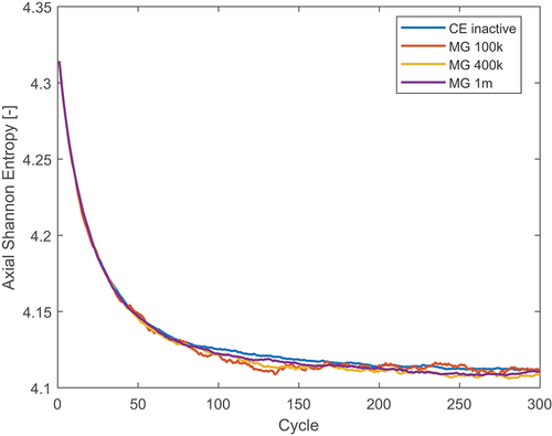
Fig. 20. Radial Shannon entropy for different neutron populations in the burnt PWR assembly with material grouping.
shows the axial reference entropy and the one calculated with 400 000 particles per cycle as a function of computational time. Contrary to the previous models, the inactive cycle speedup reaches a factor of approximately 4 or 5. Each MG cycle is nine times faster than each CE cycle. This is to be expected due to the large number of different materials and nuclides present in the geometry that largely slow down the CE calculation due to increased cross-section lookups. The net advantage of MG cross sections is therefore greater in this case.
Fig. 21. Axial Shannon entropy as a function of run time for the 400 000-neutrons/cycle case in the burnt PWR assembly with material grouping.
The axial flux profiles for the cases considered are shown in , while the relative error can be seen in . The average errors of all cases are generally within the standard deviation of the CE runs. The only exceptions are the 100 000- and 1 million–particle cases, which reach an average error of up to 2% at the bottom of the assembly. On the other hand, the error for the 400 000-particle case is below 1% in the same region. This seems to imply that the increased error when increasing the population is purely due to noise. While the standard deviation reaches up to 8% when only 100 000 particles per cycle are used, in the other cases it is strongly reduced. However, it is consistently larger than the CE standard deviation.
Fig. 22. Axial flux profile produced by different neutron populations in the burnt PWR assembly with material grouping.
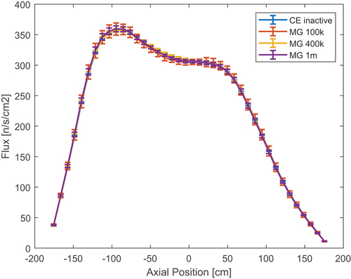
Fig. 23. Relative difference between MG and reference axial flux when using different neutron populations in the burnt PWR assembly with material grouping.
shows the reference axially integrated radial flux profile, while shows the error produced by the 400 000-particle case. Once again, the radial flux has a much lower error compared to the axial one. The MG flux is almost consistently within 0.1% of the reference one.
Fig. 24. Reference radial flux profile in the burnt PWR assembly with material grouping.
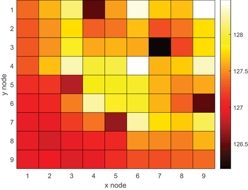
Fig. 25. Relative difference between 23-group MG (400 000 particles/cycle) and reference radial flux in the burnt PWR assembly with material grouping.
IV. SUMMARY AND CONCLUSIONS
In this paper, a novel source convergence acceleration method for Monte Carlo transport criticality calculations is proposed. The method consists of simulating most of the inactive cycles with MG cross sections. The MG cross sections can be generated at the beginning of the calculation during a few CE inactive cycles. In most cases, the MG inactive cycles converge to a slightly different fission source compared to the CE full-fidelity one. Therefore, in order to ensure proper convergence, a certain number of final CE inactive cycles can also be added. Then all the active cycles are simulated with CE as is conventional practice. This method was devised to address the problem of slow convergence in high dominance ratio reactor models.
This method was tested on three 3-D light water assembly/minireactor models. These were a PWR assembly with fresh fuel, gadolinium-bearing pins, and an axial water density profile; a CE version of the deterministic benchmark C5G7, and a PWR assembly identical to the previous one but with fuel burnt up to 10 MWd/kg. These models were chosen for their challenging features—the presence of gadolinium, MOX fuel, and burnt fuel, as well as an axial water density profile—that are meant to introduce challenging spectral effects present in realistic scenarios. For these models, Shannon entropy was used as an approximate convergence indicator, while the ultimate measure for successful convergence was the comparison of the final flux profiles of the MG case with the reference case. Other convergence estimators were not considered in this paper.
For all cases, different studies on the population parameters to be used were carried out. In general, it was found that the CASMO23 group structure could successfully be used for all models. For the models implemented, 20 generation cycles could produce cross sections with an average uncertainty around 3% for capture and fission cross sections, and 13% for the scattering matrices. The large cross-section uncertainties were found to be the most limiting aspect of the method. This is exacerbated by the fact that uncertainties do not converge following a trend in high dominance ratio problems. This implies that a prohibitively large number of cross-section generation cycles should be used to reduce uncertainties slightly. At the same time, it was found that cross sections have their maximum uncertainty at the top and at the bottom of the model, i.e., where the neutron population is the lowest. This implies that the errors propagate largely toward regions that are not particularly statistically significant. However, errors around 2% on the final flux profiles and uncertainties around 4% could easily be seen at the axial extremities. A possible solution to this problem, to be investigated in the future, is to apply the uniform fission site method.Citation22 The application of this technique has previously been shown to resoundingly reduce uncertainties in estimators located near core extremities and seems a promising and cheap means of reducing MG cross-section uncertainties (and resulting flux errors) if used alongside the present method.
Despite these issues, with a careful selection of the population parameters, all models produced satisfying results. It must be kept in mind that large dominance ratio models suffer from detrimental correlation effects that do not depend on the nuclear data type used. As a consequence, when running independent instances of the CE reference cases, standard deviations of up to 4% could be seen. The average error of the MG cases were generally within that standard deviation band. However, the standard deviation generated from independent MG runs tends to be larger than the CE one.
An additional issue arose for the burnt PWR assembly problem, when generating a separate set of cross sections per each material did not produce satisfactory results. This was a consequence of extreme uncertainties in the cross sections everywhere in the geometry; while the other cases had around 30 materials, the burnt assembly included around 400. In order to reduce statistical errors, cross sections were averaged over chosen sets of spatially separated materials. During the MG portion of the calculation, each individual material within a set used the same cross sections. This greatly reduced the cross-section uncertainties and the final error.
Memory utilization was measured only for the burnt fuel assembly model, i.e., the one with the largest number of materials. When using 23 groups and a set of cross sections per each material, memory usage increased by 17%. When grouping fuel materials together, however, memory utilization only increased by 1%.
The speedup achieved by this method ranges from a factor of around 2.5 to a factor of around 5. In particular, the highest computational gain comes in computationally expensive problems, such as the burnt fuel one. This happens because the CE calculation is heavily slowed down by the presence of more than 200 nuclides and 400 materials. However, it is clear that informed choices of parameters must be made in order to ensure appropriate results. For each calculation, the user must input the group structure to be used, the number of cross-section generation cycles, and the number of final CE inactive cycles. All of these parameters are also influenced by the neutron population per cycle. Additionally, it must be decided whether a cross-section set should be generated per each material or per some group of materials. These choices must be well informed in order not to deteriorate the calculation results. Even if all the LWR models tested produced satisfactory results with 23 groups, it is also expected that different reactor types would require different energy structures and different parameters.
While the use of arbitrary parameters is a disadvantage of the method, it must be emphasized that all source convergence acceleration methods require some arbitrary choices. To state a few examples, for convergence acceleration using CMFD, these consist of choosing an appropriate spatial mesh, energy group scheme, and the number of cycles over which to generate group constants. For the response matrix, these include the spatial mesh, number of inner and outer iterations, and the number of correcting cycles. Finally, for particle ramping, these include the ramping rate and initial number of particles. Therefore, some degree of arbitrariness is not surprising in acceleration methods. However, future work will address the problem of automating the choice of some simulation parameters, such as the switch between CE and MG inactive cycles and between inactive and active cycles.
Acknowledgments
This work was cosponsored by the United Kingdom Engineering and Physical Sciences Research Council under grant number EP/R513180/1 and by AWE.
Disclosure Statement
No potential conflict of interest was reported by the authors.
References
- F. B. BROWN, “Fundamentals of Monte Carlo Particle Transport” (2005).
- F. B. BROWN, “On the Use of Shannon Entropy of the Fission Distribution for Assessing Convergence of Monte Carlo Criticality Calculations,” Proc. PHYSOR 2006, Vancouver, British Columbia (2006).
- B. R. HERMAN, “Monte Carlo and Thermal Hydraulic Coupling Using Low-Order Nonlinear Diffusion Acceleration,” PhD Thesis, Massachusetts Institute of Technology, Department of Nuclear Science and Engineering (2014).
- E. DUMONTEIL et al., “Particle Clustering in Monte Carlo Criticality Simulations,” Ann. Nucl. Energy, 63, 612 (Jan. 2014); https://doi.org/10.1016/j.anucene.2013.09.008.
- J. LEPPÄNEN, “Acceleration of Fission Source Convergence in the Serpent 2 Monte Carlo Code Using a Response Matrix Based Solution for the Initial Source Distribution,” Ann. Nucl. Energy, 128, 63 (2019); https://doi.org/10.1016/j.anucene.2018.12.044.
- J. LEPPÄNEN et al., “The Serpent Monte Carlo Code: Status, Development and Applications in 2013,” Ann. Nucl. Energy, 82, 142 (2015); https://doi.org/10.1016/j.anucene.2014.08.024.
- M. J. LEE et al., “Coarse Mesh Finite Difference Formulation for Accelerated Monte Carlo Eigenvalue Calculation,” Ann. Nucl. Energy, 65, 101 (2014); https://doi.org/10.1016/j.anucene.2013.10.025.
- K. P. KEADY and E. W. LARSEN, “Stability of Monte Carlo k-eigenvalue Simulations with CMFD Feedback,” J. Comput. Phys., 321, 947 (2016); https://doi.org/10.1016/j.jcp.2016.06.002.
- T. J. URBATSCH, “Iterative Acceleration Methods for Monte Carlo and Deterministic Criticality Calculations,” PhD Thesis, University of Michigan, Department of Nuclear Engineering and Radiological Sciences (1995).
- A. L. LUND, P. K. ROMANO, and A. R. SIEGEL, “Accelerating Source Convergence in Monte Carlo Criticality Calculations Using a Particle Ramp-up Technique,” presented at the Int. Conf. on Mathematics & Computational Methods Applied to Nuclear Science & Engineering, Jeju, Korea (2017).
- M. A. KOWALSKI, “Variable Fidelity Monte Carlo Neutron Transport,” PhD Thesis, University of Cambridge, Department of Engineering (2020).
- V. RAFFUZZI et al., “Monte Carlo Source Convergence Acceleration by Multi-group Inactive Cycles,” presented at PHYSOR 2022 (2022).
- J. R. TRAMM and A. R. SIEGEL, “Memory Bottlenecks and Memory Contention in Multi-core Monte Carlo Transport Codes,” Int. J. High Perform. Comput. Appl., 28, 1, 04208 (2014).
- M. A. KOWALSKI et al., “SCONE: A Student-Oriented Modifiable Monte Carlo Particle Transport Framework,” presented at PHYSOR 2020, Cambridge, United Kingdom (2020).
- J. LEPPÄNEN, “Development of a New Monte Carlo Reactor Physics Code,” PhD Thesis, Helsinki University of Technology, Department of Physics (2007).
- W. BOYD et al., “Multigroup Cross-Section Generation with the OpenMC Monte Carlo Particle Transport Code,” Nucl. Technol., 205, 7, 928 (2019); https://doi.org/10.1080/00295450.2019.1571828.
- M. NOWAK et al., “Monte Carlo Power Iteration: Entropy and Spatial Correlations,” Ann. Nucl. Energy, 94, 856 (2016); https://doi.org/10.1016/j.anucene.2016.05.002.
- M. GARCÍA et al., “Validation of Serpent-SUBCHANFLOW-TRANSURANUS pin-by-pin Burnup Calculations Using Experimental Data from the Temelín II VVER-1000 Reactor,” Nucl. Eng. Technol., 53, 10, 3133 (2021); https://doi.org/10.1016/j.net.2021.04.023.
- K. WANG et al., “Analysis of BEAVRS Two-Cycle Benchmark Using RMC Based on Full Core Detailed Model,” Prog. Nucl. Energy, 98, 301 (2017); https://doi.org/10.1016/j.pnucene.2017.04.009.
- S. HARPER, “Tally Derivative Based Surrogate Models for Faster Monte Carlo Multiphysics,” PhD Thesis, Massachusetts Institute of Technology, Department of Nuclear Science and Engineering (2020).
- “Benchmark on Deterministic Transport Calculations Without Spatial Homogenisation, A 2-D/3-D MOX Fuel Assembly Benchmark,” Technical Report, Organisation for Economic Co-operation and Development (2003).
- D. J. KELLY, T. M. SUTTON, and S. C. WILSON, “MC21 Analysis of the Nuclear Energy Agency Monte Carlo Performance Benchmark Problem,” Proc. PHYSOR 2012, Pittsburgh, Pennsylvania (2012).