Convergence Properties of a Linear Diffusion-Acceleration Method for k-Eigenvalue Transport Problems

Abstract

Most methods that use low-order operators to accelerate the iterative solution of transport eigenvalue problems employ nonlinear functionals of the transport solution (such as Eddington tensors) in their low-order equations, which are themselves standard eigenvalue problems. Here, we discuss linear diffusion synthetic acceleration (DSA) for $k$-eigenvalue problems, which belongs to a family of methods that has received less attention than its nonlinear counterparts. We review the history of these linear methods as far as we know it and describe theoretical questions that to our knowledge have remained unanswered. With these methods, a low-order problem is solved after each transport step for an updated eigenvalue and an additive correction to the eigenfunction. These low-order problems are not standard eigenvalue problems, for they contain residuals as fixed sources. The low-order problems admit infinitely many solutions (updated $k$ and additive correction to the eigenfunction), and the solution that is obtained depends on the initial guess and iterative method chosen for the low-order problems. Experience has shown that when the low-order problems are solved with a powerlike iteration method and certain initial guesses, they yield solutions that cause rapid convergence to the correct high-order solution. We study the convergence properties of this algorithm applied to two model problems: an infinite homogeneous medium and a one-cell problem. For the infinite homogeneous problem, we present a Fourier analysis of the linear DSA method, which demonstrates that when the low-order problems are solved using a powerlike iteration scheme, the linear DSA scheme provides immediate convergence of the $k$-eigenvalue and rapid convergence of the eigenfunction (much like DSA applied to scattering iterations in fixed-source problems). For the one-cell problems, we find that the linear scheme for $k$-eigenvalue problems performs approximately as well as DSA for fixed-source problems. The latter analysis reveals a quantitative bound on the consistency between low- and high-order operators that is necessary and sufficient for convergence of those problems. With some theoretical foundations for the linear methods now established, we turn to numerical testing. We find, as others have before us using different low-order operators, that the method works well in practice. We provide numerical results from reactor problems in which our linear DSA is approximately as effective as the more widely used nonlinear methods. Our theoretical and numerical results add to the body of evidence that the linear methodology offers a simple path to rapid convergence of $k$-eigenvalue problems, especially for codes that already employ linear low-order operators to converge scattering iterations.

Keywords:

• Transport
• diffusion
• $k$-eigenvalue
• acceleration
• preconditioner

I. INTRODUCTION

In this paper, we discuss solution methods for the multigroup discrete ordinates $k$-eigenvalue neutron transport equation, which can be written as follows:

(1) $\left({\vec{\mathrm{\Omega }}}_m\cdot \vec{\mathrm{\nabla }}+T\right){\mathrm{\Psi }}_m=\frac{1}{4\pi }{S}_m\mathrm{\Phi }+\frac{1}{4\pi }\frac{1}{k}F{\mathrm{\Phi }}_0,m=1\dots M,$(1)

and

(2) $\mathrm{\Phi }=W\mathrm{\Psi },$(2)

where

$\mathrm{\Psi }$	=	= vector of unknowns that represent the position-, direction-, and energy-dependent neutron angular flux
$M$	=	= number of directions in the quadrature set (which can differ for different energy groups)
$\mathrm{\Phi }$	=	= vector of angular moments needed to build the scattering source
${\mathrm{\Phi }}_0$	=	= scalar flux (zeroth angular moment)
${\vec{\mathrm{\Omega }}}_m$	=	= unit vector in the m’th quadrature direction
$T$	=	= total collision operator
$S_m$	=	= transfer operator [describing scattering, (n,2n), and other nonfission neutron-emitting interactions]
$F$	=	= fission interaction operator
$W$	=	= angular-moment operator
$k$	=	= eigenvalue to be determined.

A straightforward solution method for this problem is power iteration (PI):

(3) $\left({\vec{\mathrm{\Omega }}}_m\cdot \vec{\mathrm{\nabla }}+T-\frac{1}{4\pi }W{S}_m\right){\mathrm{\Psi }}_m^{(t+1)}=\frac{1}{4\pi }\frac{1}{k^{(t)}}F{\mathrm{\Phi }}_0^{(t)},$(3)

(4) ${\mathrm{\Phi }}_0^{(t+1)}=W_0{\mathrm{\Psi }}^{(t+1)},$(4)

and

(5) $k^{(t+1)}=k^{(t)}\frac{||F{\mathrm{\Phi }}_0^{(t+1)}||}{||F{\mathrm{\Phi }}_0^{(t)}||}.$(5)

Upon convergence of the outer iteration, or PI, at index $t$, $k$ is the largest of the $k$-eigenvalues, and $\mathrm{\Psi }$ is the associated eigenfunction. As written here, each PI requires solving for ${\mathrm{\Psi }}^{(t+1)}$, which itself requires iteration. A straightforward option for this inner iteration is source iteration (SI):

(6) $\left({\vec{\mathrm{\Omega }}}_m\cdot \vec{\mathrm{\nabla }}+T\right){\mathrm{\Psi }}_m^{(i+1)}=\frac{1}{4\pi }W{S}_m{\mathrm{\Psi }}^i+\frac{1}{4\pi }\frac{1}{k^{(t)}}F{\mathrm{\Phi }}_0^{(t)},$(6)

with ${\mathrm{\Psi }}_m^{(t+1)}$ set to ${\mathrm{\Psi }}_m^{(i+1)}$ upon convergence.

The PI convergence rate depends on the eigenvalue dominance ratio, which can be arbitrarily close to 1, in which case PI converges arbitrarily slowly. (See Sec. VIII of Ref. 1.) The SI convergence rate depends on the scattering ratio (fraction of interactions that are scatters), which can also be close to 1, in which case SI converges slowly. (See Sec. II of Ref. 1.)

For many problems of practical interest, both the dominance ratio and scattering ratio are sufficiently close to 1 that it is beneficial to replace or modify both the outer and inner iteration methods to achieve faster convergence.^2–6 In this paper we consider methods that retain the basic outer/inner structure but employ low-order approximations of the transport operator to accelerate convergence. Our purpose is to help fill a gap in the theoretical foundation for a family of these methods that employ linear low-order operators.

Both linear and nonlinear low-order operators have been used effectively in $k$-eigenvalue problems. When nonlinear low-order operators are employed to accelerate convergence of outer iterations, the result is a series of low-order problems that are themselves $k$-eigenvalue problems, each with a unique largest eigenvalue and associated eigenfunction. This dominant {eigenvalue, eigenfunction} pair is the desired solution, and various techniques (including PI) can be employed to find this solution.^1–4,6–11

In contrast, when linear low-order operators are employed to accelerate convergence of outer iterations, each resulting low-order problem is not itself an eigenvalue problem, for in addition to the fission term with its $1/k$ multiplier, there is also a fixed (inhomogeneous) source term.^12–16 For this problem there is not a unique largest $k$ for which the problem has a solution. In fact, the equation admits a solution for every value of $k$ greater than a certain well-defined value. In spite of this apparent theoretical issue, all applications of the linear methodology that we know of have been successful, with iterative performance comparable to that seen with nonlinear methods. Each application that we know of has employed a powerlike iteration scheme for the eigenvalue-like low-order problem, and this powerlike iteration method apparently converges to a meaningful $k$ and associated function.

The goal of this paper is to provide theoretical foundations for methods that employ linear operators to accelerate the convergence of outer iterations in $k$-eigenvalue problems. This includes analysis of the convergence of a powerlike iteration scheme applied to the eigenvalue-like low-order problems as well as the convergence of the outer iteration (in which each iteration requires solution of a low-order eigenvalue-like problem) to the desired high-order eigenvalue and eigenfunction. Our approach is to perform convergence analyses of model problems for which we have devised analysis techniques. These problems are much simpler than real-world reactor problems, but they serve as a starting point for understanding the behavior of the iterative methods of interest here. The same kinds of simple model problems proved very helpful in the early days of understanding and developing rapidly convergent iterative methods for fixed-source problems.^1,17–20

We remark that there are many approaches to solving $k$-eigenvalue problems that do not employ low-order operators in the way described above. These include subspace methods (Arnoldi iteration, Chebyshev iteration),^21,22 casting the eigenvalue problem as a nonlinear partial differential equation constraint problem and solving using a nonlinear solver such as a Newton-like method, and treating part of the fission source implicitly to reduce the dominance ratio (Wielandt shift). We do not address these methods here but will mention that acceleration using low-order operators has been shown to improve these methods as well.^16,23

In Sec. II, we describe the linear low-order methodology, including its developmental history as we understand it, and illustrate it using $P_1$ as the low-order approximation for transport. We compare and contrast this to the nonlinear low-order methodology, using quasi-diffusion as the example. In Sec. III, we present convergence analyses for two model problems. The first model problem employs transport and diffusion operators without spatial discretization and applies them to a one-energy-group problem in an infinite homogeneous medium. The second model problem employs spatial discretization for the transport and low-order operators and applies the method to a single-cell problem with vacuum boundaries. We close the section with a discussion of spatial discretization considerations. In Sec. IV, we present numerical results from reactor test problems including those with strong heterogeneities, fine spatial features, large numbers of spatial cells, and large numbers of energy unknowns. We offer conclusions in Sec. V.

II. LINEAR SYNTHETIC ACCELERATION FOR EIGENFUNCTION CORRECTION AND UPDATED EIGENVALUE

II.A. Description and History

In what follows, we use equations without spatial discretization for illustration. The family of methods we study here employ nested iterations. If we let $(t)$ be the index of the outermost iteration and $(i)$ be the index of the scattering iteration, then the methods we consider have the following at the end of the transport portion of the t’th iteration:

(7) $\left({\vec{\mathrm{\Omega }}}_m\cdot \vec{\mathrm{\nabla }}+T\right){\mathrm{\Psi }}_m^{(i+1)}=\frac{1}{4\pi }\left(\begin{array}{c}{S}_{m,con}{\mathrm{\Phi }}^{(i+1)}+S_{m,rec}{\mathrm{\Phi }}^{(i+1/2)}\\ +S_{m,lag}{\mathrm{\Phi }}^{(i)}+\frac{1}{k^{(t)}}F{\mathrm{\Phi }}_0^{(t)}\end{array}\right),$(7)

where

${\mathrm{\Psi }}_m$	=	= vector containing the angular flux for all energy groups for direction $m$
$\mathrm{\Phi }$	=	= vector containing all the angular moments needed to form the scattering source for all groups
${\mathrm{\Phi }}_0$	=	= vector of scalar fluxes for all groups
$\frac{1}{4\pi }{S}_{m,con}{\mathrm{\Phi }}^{(i+1)}$	=	= scattering source rate density for direction $m$ that has been previously determined (e.g., downscattering from fast groups)
$\frac{1}{4\pi }{S}_{m,rec}{\mathrm{\Phi }}^{(i+1/2)}$	=	= scattering source rate density for direction $m$ that has been updated from the most recent transport step (iteration index $i+1/2$, e.g., within-group scattering)
$\frac{1}{4\pi }{S}_{m,lag}{\mathrm{\Phi }}^{(i)}$	=	= scattering source rate density for direction $m$ that is evaluated at a previous iterate (e.g., upscattering)
$\frac{1}{4\pi }\frac{1}{k^{(t)}}F{\mathrm{\Phi }}_0^{(t)}$	=	= fission source rate density

and $T$ contains the total cross section for each group.

The total scattering is equal to the sum of the converged, recent, and lagged components of scattering:

(8) $S_m=S_{m,con}+S_{m,rec}+S_{m,lag}.$(8)

As far as we know, the first derivation, implementation, and testing of a method in the family considered here appeared in a 1986 dissertation.¹² The author developed eigenproblem acceleration equations via a process that previous researchers had employed for scattering iterations: (1) Define “converged” equations by setting all iteration indices to the same value; (2) subtract the equations satisfied by the latest solution, obtaining an exact equation for an additive correction; (3) replace the transport operator in this equation by a low-order operator. In the notation of this paper, the first step produces

(9) $\left({\vec{\mathrm{\Omega }}}_m\cdot \vec{\mathrm{\nabla }}+T\right){\mathrm{\Psi }}_m^{(t+1)}=\frac{1}{4\pi }\left(\begin{array}{c}{S}_{m,con}{\mathrm{\Phi }}^{(t+1)}+S_{m,rec}{\mathrm{\Phi }}^{(t+1)}\\ +S_{m,lag}{\mathrm{\Phi }}^{(t+1)}+\frac{F{\mathrm{\Phi }}_0^{(t+1)}}{k^{(t+1)}}\end{array}\right).$(9)

The second step subtracts Eq. (7)(7) $\left({\vec{\mathrm{\Omega }}}_m\cdot \vec{\mathrm{\nabla }}+T\right){\mathrm{\Psi }}_m^{(i+1)}=\frac{1}{4\pi }\left(\begin{array}{c}{S}_{m,con}{\mathrm{\Phi }}^{(i+1)}+S_{m,rec}{\mathrm{\Phi }}^{(i+1/2)}\\ +S_{m,lag}{\mathrm{\Phi }}^{(i)}+\frac{1}{k^{(t)}}F{\mathrm{\Phi }}_0^{(t)}\end{array}\right),$(7) from this converged equation. We define $y^{(t+1)}={\mathrm{\Psi }}^{(t+1)}-{\mathrm{\Psi }}^{(i+1)}$, $f^{(t+1)}={\mathrm{\Phi }}^{(t+1)}-{\mathrm{\Phi }}^{(i+1)}$, and $f_0^{(t+1)}={\mathrm{\Phi }}_0^{(t+1)}-{\mathrm{\Phi }}_0^{(i+1)}$. Then, we have

(10) $\left({\vec{\mathrm{\Omega }}}_m\cdot \vec{\mathrm{\nabla }}+T\right)y_m^{(t+1)}=\frac{1}{4\pi }\left(\begin{array}{c}{S}_m{f}^{(t+1)}+\frac{F\left(f_0^{(t+1)}+{\mathrm{\Phi }}_0^{(i+1)}\right)}{k^{(t+1)}}\\ +R_m^{(i+1)}\end{array}\right),$(10)

where

(11) $R_m^{(i+1)}\equiv S_{m,rec}\left({\mathrm{\Phi }}^{(i+1)}-{\mathrm{\Phi }}^{(i+1/2)}\right)+S_{m,lag}\left({\mathrm{\Phi }}^{(i+1)}-{\mathrm{\Phi }}^{(i)}\right)-\frac{1}{k^{(t)}}F{\mathrm{\Phi }}_0^{(t)}.$(11)

The third step replaces the transport operator with a low-order operator, which for Adams was a diffusion operator.¹² We illustrate with a $P_1$ operator:

(12) $\overrightarrow{\nabla }\cdot {\overrightarrow{g}}^{(t+1)}+\left(T-S_0\right)f_0^{(t+1)}=\frac{1}{k^{(t+1)}}F\left({\Phi }_0^{(i+1)}+f_0^{(t+1)}\right)+R_0^{(i+1)}\text{},$(12)

and

(13) $\frac{1}{3}\vec{\mathrm{\nabla }}\cdot f_0^{(t+1)}+T{\vec{g}}^{(t+1)}=S_1{\vec{g}}^{(t+1)}+{\vec{R}}_1^{(i+1)},$(13)

where $R_0$ and ${\vec{R}}_1$ are the zeroth and first angular moments of $R_m/4\pi$ and the correction to the currents is defined as ${\vec{g}}^{(t+1)}={\vec{J}}^{(t+1)}-{\vec{J}}^{(i+1)}$.

Finally, an iterative method must be defined to solve for the new eigenvalue $k^{(t+1)}$ and eigenfunction additive correction $f_0^{(t+1)}$. An obvious choice, and the one made by Adams,¹² is a process that resembles PI, with starting guesses $f_0^{(0)}=0$ and $k^{(n)}{|}_{n=0}=k^{(t)}$:

(14) $\vec{\mathrm{\nabla }}\cdot {\vec{g}}^{(n+1)}+(T-S_0)f_0^{(n+1)}=\frac{1}{k^{(n)}}F({\mathrm{\Phi }}_0^{(i+1)}+f_0^{(n)})+R_0^{(i+1)},$(14)

(15) $\frac{1}{3}\vec{\mathrm{\nabla }}\cdot f_0^{(n+1)}+T{\vec{g}}^{(n+1)}=S_1{\vec{g}}^{(n+1)}+{\vec{R}}_1^{(i+1)},$(15)

and

(16) $k^{(n+1)}=k^{(n)}\frac{∥F(f_0^{(n+1)}+{\mathrm{\Phi }}_0^{(i+1)})∥}{∥F(f_0^{(n)}+{\mathrm{\Phi }}_0^{(i+1)})∥}.$(16)

Upon convergence, this low-order eigenvalue-like problem yields the next eigenvalue and eigenfunction iterates:

(17) $k^{(t+1)}\leftarrow k^{(n+1)}\mathrm{a}\mathrm{n}\mathrm{d}{\mathrm{\Phi }}_0^{(t+1)}\leftarrow {\mathrm{\Phi }}_0^{(i+1)}+f_0^{(t+1)}.$(17)

While the aforementioned 1986 dissertation reported excellent results, the method remained unpublicized because of theoretical concerns. It was observed that given the presence of the fixed source in Eq. (12(12) $\overrightarrow{\nabla }\cdot {\overrightarrow{g}}^{(t+1)}+\left(T-S_0\right)f_0^{(t+1)}=\frac{1}{k^{(t+1)}}F\left({\Phi }_0^{(i+1)}+f_0^{(t+1)}\right)+R_0^{(i+1)}\text{},$(12) ) ($R_0$ plus part of the fission source), it is not clear that the low-order problem will always yield a helpful solution. For example, one could set $k^{(t+1)}$ to some arbitrary large value and solve the resulting fixed-source subcritical diffusion problem for the associated $f$. Setting a different value for $k^{(t+1)}$ would produce a different function for $f$. That is, infinitely many solutions ($k$ and $f$) that are unrelated to the eigenproblem of interest are seen to satisfy Eqs. (12)(12) $\overrightarrow{\nabla }\cdot {\overrightarrow{g}}^{(t+1)}+\left(T-S_0\right)f_0^{(t+1)}=\frac{1}{k^{(t+1)}}F\left({\Phi }_0^{(i+1)}+f_0^{(t+1)}\right)+R_0^{(i+1)}\text{},$(12) and (13)(13) $\frac{1}{3}\vec{\mathrm{\nabla }}\cdot f_0^{(t+1)}+T{\vec{g}}^{(t+1)}=S_1{\vec{g}}^{(t+1)}+{\vec{R}}_1^{(i+1)},$(13) .

Numerical tests indicated that when the specific iteration process and initial guesses defined above were followed, the method worked quite well. Nevertheless, the absence of a theoretical understanding left a concern that the method might fail on some problems (for example, if the low-order powerlike iteration failed to converge or converged to some additive correction that degraded instead of improved the latest transport solution). We remark that Adams and Larsen did publish a related linear method that was shown to converge rapidly, but it was defined only for the one-group case.¹³

Later, Suslov independently created the same basic method (with a different low-order operator) and provided an argument for why one would expect the low-order problem to converge to a useful solution.¹⁴ We paraphrase Suslov’s argument as follows, including only the zeroth moment scattering for simplicity. In operator notation, Eqs. (7)(7) $\left({\vec{\mathrm{\Omega }}}_m\cdot \vec{\mathrm{\nabla }}+T\right){\mathrm{\Psi }}_m^{(i+1)}=\frac{1}{4\pi }\left(\begin{array}{c}{S}_{m,con}{\mathrm{\Phi }}^{(i+1)}+S_{m,rec}{\mathrm{\Phi }}^{(i+1/2)}\\ +S_{m,lag}{\mathrm{\Phi }}^{(i)}+\frac{1}{k^{(t)}}F{\mathrm{\Phi }}_0^{(t)}\end{array}\right),$(7) , (14(14) $\vec{\mathrm{\nabla }}\cdot {\vec{g}}^{(n+1)}+(T-S_0)f_0^{(n+1)}=\frac{1}{k^{(n)}}F({\mathrm{\Phi }}_0^{(i+1)}+f_0^{(n)})+R_0^{(i+1)},$(14) ), and (15(15) $\frac{1}{3}\vec{\mathrm{\nabla }}\cdot f_0^{(n+1)}+T{\vec{g}}^{(n+1)}=S_1{\vec{g}}^{(n+1)}+{\vec{R}}_1^{(i+1)},$(15) ) are

(18) $A{\Phi }_0^{(i+1)}=-R_0^{(i+1)},$(18)

and

(19) $B{f}_0^{(n+1)}=\frac{1}{k^{(n)}}F\left({\mathrm{\Phi }}_0^{(i+1)}+f_0^{(n)}\right)+R_0^{(i+1)},$(19)

Adding these two equations gives

(20) $A{\mathrm{\Phi }}_0^{(i+1)}+B{f}_0^{(n+1)}=\frac{1}{k^{(n)}}F\left({\mathrm{\Phi }}_0^{(i+1)}+f_0^{(n)}\right).$(20)

If we had $B=A$ (low-order = high-order), then this method would be equivalent to solving a standard eigenvalue equation for the next eigenfunction iterate. That is, even though Eq. (19)(19) $B{f}_0^{(n+1)}=\frac{1}{k^{(n)}}F\left({\mathrm{\Phi }}_0^{(i+1)}+f_0^{(n)}\right)+R_0^{(i+1)},$(19) does admit solutions that are not related to the eigenproblem, as Larsen had observed, solving it using a powerlike iteration is algebraically equivalent to solving a problem—Eqs. (20)(20) $A{\mathrm{\Phi }}_0^{(i+1)}+B{f}_0^{(n+1)}=\frac{1}{k^{(n)}}F\left({\mathrm{\Phi }}_0^{(i+1)}+f_0^{(n)}\right).$(20) and (16(16) $k^{(n+1)}=k^{(n)}\frac{∥F(f_0^{(n+1)}+{\mathrm{\Phi }}_0^{(i+1)})∥}{∥F(f_0^{(n)}+{\mathrm{\Phi }}_0^{(i+1)})∥}.$(16) )—that has no fixed source and is similar to (but if $B\ne A$ not quite the same as) a standard eigenvalue problem. Thus, Suslov justified using a low-order transport operator for $B$ and reported excellent results.¹⁴

Masiello and Rossi have also reported excellent results from the application of a method in the family of linear acceleration schemes that we study here for $k$-eigenvalue problems.¹⁵ They applied the boundary-projection acceleration (BPA) low-order operator to multigroup $k$-eigenvalue discrete ordinates problems with anisotropic scattering.²⁰ They presented a Fourier analysis of the iterative convergence rate of their BPA method for fixed-source problems, providing a sound theoretical basis for the application of BPA to such problems. They did not present theoretical analysis of convergence of the method for eigenvalue problems, but they provided results that demonstrated excellent performance.

II.B. Theoretical Questions

Theoretical questions remain if $B\ne A$. If an operator $C$ existed such that

(21) $A{\mathrm{\Phi }}_0^{(i+1)}+B{f}_0^{(n+1)}=C\left({\mathrm{\Phi }}_0^{(i+1)}+f_0^{(n+1)}\right)$(21)

for all possible $f_0^{(n+1)}$, then the given iteration method would be algebraically equivalent to PI on the operator $C^{-1}F$. This would find the largest eigenvalue and the associated eigenfunction, and the only theoretical question would be how rapidly this well-posed low-order problem would accelerate the overall iteration.

We now show that given the $A$ and $B$ operators studied here, there does exist an operator $C^{(n+1)}$ such that $A{\mathrm{\Phi }}_0^{(i+1)}+B{f}_0^{(n+1)}=C^{(n+1)}({\mathrm{\Phi }}_0^{(i+1)}+f_0^{(n+1)})$. However, this operator depends on $f_0^{(n+1)}$ and thus changes from iteration to iteration. If we take the zeroth and first angular moments of Eq. (7(7) $\left({\vec{\mathrm{\Omega }}}_m\cdot \vec{\mathrm{\nabla }}+T\right){\mathrm{\Psi }}_m^{(i+1)}=\frac{1}{4\pi }\left(\begin{array}{c}{S}_{m,con}{\mathrm{\Phi }}^{(i+1)}+S_{m,rec}{\mathrm{\Phi }}^{(i+1/2)}\\ +S_{m,lag}{\mathrm{\Phi }}^{(i)}+\frac{1}{k^{(t)}}F{\mathrm{\Phi }}_0^{(t)}\end{array}\right),$(7) ), we see that Eqs. (22)(22) $\overrightarrow{\nabla }\cdot {\overrightarrow{J}}^{(i+1)}+T{\Phi }_0^{(i+1)}=S_0{\Phi }_0^{(i+1)}-R_0^{(i+1)},$(22) , (23(23) $\overrightarrow{\nabla }\cdot {\overrightarrow{\overrightarrow{P}}}^{(i+1)}+T{\overrightarrow{J}}^{(i+1)}=S_1{\overrightarrow{J}}^{(i+1)}-{\overrightarrow{R}}_1^{(i+1)},$(23) ), and (24(24) $\overrightarrow{J}\equiv {\displaystyle \sum _m{w}_m}{\overrightarrow{\Omega }}_m{\Psi }_m,\overrightarrow{\overrightarrow{P}}\equiv {\displaystyle \sum _m{w}_m}{\overrightarrow{\Omega }}_m{\overrightarrow{\Omega }}_m{\Psi }_m,$(24) ) are satisfied at the end of the transport step:

(22) $\overrightarrow{\nabla }\cdot {\overrightarrow{J}}^{(i+1)}+T{\Phi }_0^{(i+1)}=S_0{\Phi }_0^{(i+1)}-R_0^{(i+1)},$(22)

and

(23) $\overrightarrow{\nabla }\cdot {\overrightarrow{\overrightarrow{P}}}^{(i+1)}+T{\overrightarrow{J}}^{(i+1)}=S_1{\overrightarrow{J}}^{(i+1)}-{\overrightarrow{R}}_1^{(i+1)},$(23)

where

(24) $\overrightarrow{J}\equiv {\displaystyle \sum _m{w}_m}{\overrightarrow{\Omega }}_m{\Psi }_m,\overrightarrow{\overrightarrow{P}}\equiv {\displaystyle \sum _m{w}_m}{\overrightarrow{\Omega }}_m{\overrightarrow{\Omega }}_m{\Psi }_m,$(24)

and subscripts $0$ and $1$ refer to zeroth and first angular moments. We define an Eddington tensor using the latest transport information, ${\overrightarrow{\overrightarrow{E}}}^{(i+1)}\equiv {\overrightarrow{\overrightarrow{P}}}^{(i+1)}/{\Phi }_0^{(i+1)}$, and then add Eqs. (14)(14) $\vec{\mathrm{\nabla }}\cdot {\vec{g}}^{(n+1)}+(T-S_0)f_0^{(n+1)}=\frac{1}{k^{(n)}}F({\mathrm{\Phi }}_0^{(i+1)}+f_0^{(n)})+R_0^{(i+1)},$(14) and (15(15) $\frac{1}{3}\vec{\mathrm{\nabla }}\cdot f_0^{(n+1)}+T{\vec{g}}^{(n+1)}=S_1{\vec{g}}^{(n+1)}+{\vec{R}}_1^{(i+1)},$(15) ) to Eqs. (22)(22) $\overrightarrow{\nabla }\cdot {\overrightarrow{J}}^{(i+1)}+T{\Phi }_0^{(i+1)}=S_0{\Phi }_0^{(i+1)}-R_0^{(i+1)},$(22) and (23(23) $\overrightarrow{\nabla }\cdot {\overrightarrow{\overrightarrow{P}}}^{(i+1)}+T{\overrightarrow{J}}^{(i+1)}=S_1{\overrightarrow{J}}^{(i+1)}-{\overrightarrow{R}}_1^{(i+1)},$(23) ) to obtain

(25) $\vec{\mathrm{\nabla }}\cdot \left({\vec{J}}^{(i+1)}+{\vec{g}}^{(n+1)}\right)+\left(T-S_0\right)\left({\mathrm{\Phi }}_0^{(i+1)}+f_0^{(n+1)}\right)=\frac{1}{k^{(n)}}F\left({\mathrm{\Phi }}_0^{(i+1)}+f_0^{(n)}\right)$(25)

and

(26) $\overrightarrow{\nabla }\cdot \left({\overrightarrow{\overrightarrow{E}}}^{(i+1)}{\Phi }_0^{(i+1)}+\frac{1}{3}\overrightarrow{\overrightarrow{I}}{f}_0^{(n+1)}\right)+(T-S_1)\left({\overrightarrow{J}}^{(i+1)}+{\overrightarrow{g}}^{(n+1)}\right)=0,$(26)

where $\overrightarrow{\overrightarrow{I}}$ is the identity tensor. We define a new tensor ${\overrightarrow{\overrightarrow{M}}}^{(n+1)}$ that is a weighted average of $\overrightarrow{\overrightarrow{I}}/3$ and the Eddington tensor from the the latest transport step using the diffusion correction and transport scalar flux as weights:

(27) ${\overrightarrow{\overrightarrow{M}}}^{(n+1)}\equiv \frac{\left({\overrightarrow{\overrightarrow{E}}}^{(i+1)}{\Phi }_0^{(i+1)}+\frac{1}{3}\overrightarrow{\overrightarrow{I}}{f}_0^{(n+1)}\right)}{{\Phi }_0^{(i+1)}+f_0^{(n+1)}}.$(27)

We also define the latest ${\mathrm{\Phi }}_0$ and $\vec{J}$ quantities:

(28) ${\mathrm{\Phi }}_0^{(n+1)}\equiv {\mathrm{\Phi }}_0^{(i+1)}+f_0^{(n+1)}\mathrm{a}\mathrm{n}\mathrm{d}{\vec{J}}^{(n+1)}\equiv {\vec{J}}^{(i+1)}+{\vec{g}}^{(n+1)}.$(28)

Then, we see that our low-order $k$ iteration scheme satisfies Eqs. (29)(29) $\vec{\mathrm{\nabla }}\cdot {\vec{J}}^{(n+1)}+\left(T-S_0\right){\mathrm{\Phi }}_0^{(n+1)}=\frac{1}{k^{(n)}}F{\mathrm{\Phi }}_0^{(n)},$(29) , (30)(30) $\overrightarrow{\nabla }\cdot \left({\overrightarrow{\overrightarrow{M}}}^{(n+1)}{\Phi }_0^{(n+1)}\right)+\left(T-S_1\right){\overrightarrow{J}}^{(n+1)}=0,$(30) , and (31)(31) $k^{(n+1)}=k^{(n)}\frac{∥F{\mathrm{\Phi }}_0^{(n+1)}∥}{∥F{\mathrm{\Phi }}_0^{(n)}∥}.$(31) :

(29) $\vec{\mathrm{\nabla }}\cdot {\vec{J}}^{(n+1)}+\left(T-S_0\right){\mathrm{\Phi }}_0^{(n+1)}=\frac{1}{k^{(n)}}F{\mathrm{\Phi }}_0^{(n)},$(29)

(30) $\overrightarrow{\nabla }\cdot \left({\overrightarrow{\overrightarrow{M}}}^{(n+1)}{\Phi }_0^{(n+1)}\right)+\left(T-S_1\right){\overrightarrow{J}}^{(n+1)}=0,$(30)

and

(31) $k^{(n+1)}=k^{(n)}\frac{∥F{\mathrm{\Phi }}_0^{(n+1)}∥}{∥F{\mathrm{\Phi }}_0^{(n)}∥}.$(31)

This method looks like PI, in particular, the PI for the inner iteration of a quasi-diffusion method, except that the tensor ${\overrightarrow{\overrightarrow{M}}}^{(n+1)}$ changes every iteration. A few remarks are in order:

1. While this is not a true eigenvalue problem, it is similar to problems and solution methods that arise in multiphysics simulations, in which neutronics operators change as temperatures and densities change during the overall multiphysics iterative solution.

2. The change in $\overrightarrow{\overrightarrow{M}}$ from iteration to iteration is small when the correction $f_0$ is small relative to the solution ${\mathrm{\Phi }}_0$, as is the case when the overall iteration is almost converged. In this limit the powerlike iteration becomes algebraically equivalent to standard PI, which will converge.

3. The change in $\overrightarrow{\overrightarrow{M}}$ from iteration to iteration may not be small during the first overall iteration or two if the correction $f_0$ is not small relative to ${\mathrm{\Phi }}_0^{(i+1)}$. We do not know of a proof that the iteration given by Eqs. (29)(29) $\vec{\mathrm{\nabla }}\cdot {\vec{J}}^{(n+1)}+\left(T-S_0\right){\mathrm{\Phi }}_0^{(n+1)}=\frac{1}{k^{(n)}}F{\mathrm{\Phi }}_0^{(n)},$(29) , (30(30) $\overrightarrow{\nabla }\cdot \left({\overrightarrow{\overrightarrow{M}}}^{(n+1)}{\Phi }_0^{(n+1)}\right)+\left(T-S_1\right){\overrightarrow{J}}^{(n+1)}=0,$(30) ), and (31(31) $k^{(n+1)}=k^{(n)}\frac{∥F{\mathrm{\Phi }}_0^{(n+1)}∥}{∥F{\mathrm{\Phi }}_0^{(n)}∥}.$(31) ) will converge in such a case.

4. In the limit as $f_0\to 0$, ${\overrightarrow{\overrightarrow{M}}}^{(n+1)}\to {\overrightarrow{\overrightarrow{E}}}^{i+1}$. In this limit, this method produces precisely the quasi-diffusion method, which does not change as the $n$ iteration proceeds and has been shown to be rapidly convergent.

5. The arguments presented here depend on a powerlike iteration method being used for the low-order problem. It is not clear that these arguments would apply if a different solution technique were used to solve Eqs. (12)(12) $\overrightarrow{\nabla }\cdot {\overrightarrow{g}}^{(t+1)}+\left(T-S_0\right)f_0^{(t+1)}=\frac{1}{k^{(t+1)}}F\left({\Phi }_0^{(i+1)}+f_0^{(t+1)}\right)+R_0^{(i+1)}\text{},$(12) and (13(13) $\frac{1}{3}\vec{\mathrm{\nabla }}\cdot f_0^{(t+1)}+T{\vec{g}}^{(t+1)}=S_1{\vec{g}}^{(t+1)}+{\vec{R}}_1^{(i+1)},$(13) ). Given our previous observation that infinitely many solutions exist to these equations, it seems all but certain that different iterative techniques would find different solutions.

In Sec. III, we analyze the convergence behavior of the eigenvalues and eigenvectors of the two-step iteration process for simple model problems. We attempt to provide theoretical foundations to answer (1) whether the powerlike iteration applied to the low-order eigenvalue-plus-source problem converges and, if that problem converges, (2) how the low-order solution affects the rate at which the transport eigenvalue iteration converges.

III. CONVERGENCE ANALYSIS

III.A. Fourier Analysis of Infinite Homogeneous Model Problem

We analyze a particular application of the linear low-order method in which we perform one transport sweep per low-order diffusion problem solution. In the literature and our own experience, this “one-sweep” method has shown the most reduction to the total solution time. We apply this method to an infinite, homogeneous medium with isotropic scattering to determine the convergence rate of both the powerlike iteration applied to the low-order eigenvalue-plus-source problem and the convergence rate of the transport eigenvalue iteration.

The infinite homogeneous medium problem has been studied extensively to gain insight into the behavior of methods for iterating on the scattering source in fixed-source problems.¹ To our knowledge, the analysis presented below is the first to use this problem to study the behavior of linear methods for eigenvalue iterations.

For infinite homogeneous fixed-source problems, the analysis shows that the slowest converging mode without acceleration is spatially flat and isotropic in angle. One reason a low-order diffusion operator is an effective preconditioner is that it is exact for this mode. The same is true in the $k$-eigenvalue problem. The Fourier analysis for fixed-source problems with diffusion synthetic acceleration (DSA) shows that the flat, isotropic mode converges in one iteration. However, the Fourier analysis also shows the rate at which other modes converge and thus shows the overall rate of convergence of the method. As we will see below, the same is true for the $k$-eigenvalue problem.

Because we perform only one sweep per outer iteration and because there is only within-group scattering in the one-group problem, we write our transport iteration equation with only one iteration index. We denote the lack of group dependence with different symbols (${\mathrm{\Psi }}_m\equiv {\psi }_m,{\mathrm{\Phi }}_m\equiv {\varphi }_m$, $T\equiv {\sigma }_t$, $S_m\equiv {\sigma }_s$, $F\equiv \nu {\sigma }_f$) and change of iteration index [$(i+1)\equiv (i+1/2)$, $(t)\equiv (i)$]. The one-group, one-sweep transport equation is then given by the following:

(32) $\left({\vec{\mathrm{\Omega }}}_m\cdot \vec{\mathrm{\nabla }}+{\sigma }_t\right){\psi }_m^{(i+1/2)}=\frac{1}{4\pi }\left({\sigma }_s+\frac{\nu {\sigma }_f}{k^{(i)}}\right){\varphi }_0^{(i)}.$(32)

We also derive the one-group diffusion problem that follows from Eqs. (14)(14) $\vec{\mathrm{\nabla }}\cdot {\vec{g}}^{(n+1)}+(T-S_0)f_0^{(n+1)}=\frac{1}{k^{(n)}}F({\mathrm{\Phi }}_0^{(i+1)}+f_0^{(n)})+R_0^{(i+1)},$(14) and (15(15) $\frac{1}{3}\vec{\mathrm{\nabla }}\cdot f_0^{(n+1)}+T{\vec{g}}^{(n+1)}=S_1{\vec{g}}^{(n+1)}+{\vec{R}}_1^{(i+1)},$(15) ), where we have solved the first moment equation analytically and substituted the resulting Ficks law equation into ${\vec{g}}^{n+1}:$

(33) $\left(-\frac{1}{3{\sigma }_t}{\vec{\mathrm{\nabla }}}^2+{\sigma }_a\right)f_0^{(i+1/2,n+1)}=\frac{\nu {\sigma }_f}{k^{(i+1/2,n)}}\left({\tilde{\varphi }}_0^{(i+1/2,n)}\right)+R_0^{(i+1/2)},$(33)

where the low-order corrected unknown ${\tilde{\varphi }}_0^{i+1/2,n}$ is defined as

(34) ${\tilde{\varphi }}_0^{(i+1/2,n)}=\left({\varphi }_0^{(i+1/2)}+f_0^{(i+1/2,n)}\right),$(34)

and again, the residual source is

(35) $R_0^{(i+1/2)}=-\frac{\nu {\sigma }_f}{k^{(i)}}{\varphi }_0^{(i)}+{\sigma }_s\left({\varphi }_0^{(i+1/2)}-{\varphi }_0^{(i)}\right).$(35)

Similar to Eq. (20(20) $A{\mathrm{\Phi }}_0^{(i+1)}+B{f}_0^{(n+1)}=\frac{1}{k^{(n)}}F\left({\mathrm{\Phi }}_0^{(i+1)}+f_0^{(n)}\right).$(20) ), we add the zeroth moment of the one-group transport equation in Eq. (32(32) $\left({\vec{\mathrm{\Omega }}}_m\cdot \vec{\mathrm{\nabla }}+{\sigma }_t\right){\psi }_m^{(i+1/2)}=\frac{1}{4\pi }\left({\sigma }_s+\frac{\nu {\sigma }_f}{k^{(i)}}\right){\varphi }_0^{(i)}.$(32) ),

(36) $\vec{\mathrm{\nabla }}\cdot {\vec{J}}^{(i+1/2)}+{\sigma }_a{\varphi }_0^{(i+1/2)}=-R_0^{(i+1/2)},$(36)

to the diffusion equation in Eq. (33(33) $\left(-\frac{1}{3{\sigma }_t}{\vec{\mathrm{\nabla }}}^2+{\sigma }_a\right)f_0^{(i+1/2,n+1)}=\frac{\nu {\sigma }_f}{k^{(i+1/2,n)}}\left({\tilde{\varphi }}_0^{(i+1/2,n)}\right)+R_0^{(i+1/2)},$(33) ),

(37) $\vec{\mathrm{\nabla }}\cdot {\vec{J}}^{(i+1/2)}+\left(-\frac{1}{3{\sigma }_t}{\vec{\mathrm{\nabla }}}^2\right)f_0^{(i+1/2,n+1)}+{\sigma }_a{\varphi }_0^{(i+1/2)}+{\sigma }_a{f}_0^{(i+1/2,n+1)}=\frac{\nu {\sigma }_f}{k^{(i+1/2,n)}}{\tilde{\varphi }}_0^{(i+1/2,n)}.$(37)

We add $\left(-\frac{1}{3{\sigma }_t}{\vec{\mathrm{\nabla }}}^2\right){\varphi }_0^{(i+1/2)}$ to both sides and use the definition for ${\tilde{\varphi }}^{i+1/2,n+1}$ to obtain an equivalent equation that is a powerlike iteration for a diffusion operator:

(38) $\left(-\frac{1}{3{\sigma }_t}{\vec{\mathrm{\nabla }}}^2+{\sigma }_a\right){\tilde{\varphi }}_0^{(i+1/2,n+1)}=\frac{\nu {\sigma }_f}{k^{(i+1/2,n)}}{\tilde{\varphi }}_0^{(i+1/2,n)}+Q_L^{(i+1/2)},$(38)

where

(39) $Q_L^{(i+1/2)}=\left(-\frac{1}{3{\sigma }_t}{\vec{\mathrm{\nabla }}}^2{\varphi }_0^{(i+1/2)}-\vec{\mathrm{\nabla }}\cdot {\vec{J}}^{(i+1/2)}\right).$(39)

Now that we have obtained equations in a form that will be more easy to manipulate, we express the transport unknowns as Fourier integrals,

(40) ${\psi }_m^{(i+1/2)}={\displaystyle \underset{-\infty }{\overset{\infty }{\int }}d}\lambda {\psi }_{m,}\left(\overrightarrow{\lambda }\right){\omega }_H^i{e}^{i{\sigma }_t\overrightarrow{\lambda }\cdot \overrightarrow{r}},$(40)

and

(41) ${\varphi }_0^{(i)}=\underset{-\mathrm{\infty }}{\overset{\mathrm{\infty }}{\int }}d\lambda {\varphi }_{0,†}\left(\vec{\lambda }\right){\omega }_H^i{e}^{\mathbf{i}{\sigma }_t\vec{\lambda }\cdot \vec{r}},$(41)

and the low-order correction and corrected unknown as Fourier integrals,

(42) $f^{(i+1/2,n)}={\displaystyle \underset{-\infty }{\overset{\infty }{\int }}d}\lambda f_{ }\left(\overrightarrow{\lambda }\right){\omega }_L^n{e}^{i{\sigma }_t\overrightarrow{\lambda }\cdot \overrightarrow{r}},$(42)

and

(43) ${\tilde{\varphi }}_0^{(i+1/2,n)}=\underset{-\mathrm{\infty }}{\overset{\mathrm{\infty }}{\int }}d\lambda {\tilde{\varphi }}_{0,†}\left(\vec{\lambda }\right){\omega }_L^n{e}^{\mathbf{i}{\sigma }_t\vec{\lambda }\cdot \vec{r}},$(43)

where ${\omega }_H$ and ${\omega }_L$ are constants that describe the error reduction per iteration of the high-order system and low-order system, respectively. The linear independence of each mode implies a separate equation for each $\vec{\lambda }$. That is, each mode evolves independently.

After substituting the Fourier integrals, the high-order equation implies

(44) $\left(\mathbf{i}{\vec{\mathrm{\Omega }}}_m\cdot \vec{\lambda }+1\right){\sigma }_t{\psi }_{m,†}^{(i+1/2)}\left(\vec{\lambda }\right)=\frac{1}{4\pi }\left({\sigma }_s+\frac{\nu {\sigma }_f}{k^{(i)}}\right){\varphi }_{0,†}^{(i)}\left(\vec{\lambda }\right),$(44)

and the low-order equation implies

(45) $\left(\frac{1}{3}{\left|\vec{\lambda }\right|}^2{\sigma }_t+{\sigma }_a\right){\tilde{\varphi }}_{†,0}^{(i+1/2,n+1)}\left(\vec{\lambda }\right)=\frac{\nu {\sigma }_f}{k^{(i+1/2,n)}}{\tilde{\varphi }}_{†,0}^{(i+1/2,n)}\left(\vec{\lambda }\right)+Q_{L,†}^{(i+1/2)}\left(\vec{\lambda }\right).$(45)

We invert the high-order operator for each Fourier mode to determine ${\psi }_{m,†}^{i+1/2}\left(\vec{\lambda }\right):$

(46) $\begin{array}{cc}{\psi }_{m,†}^{(i+1/2)}\left(\vec{\lambda }\right)& =\frac{1}{4\pi }\frac{1}{1+\mathbf{i}{\vec{\mathrm{\Omega }}}_m\cdot \vec{\lambda }}\frac{1}{{\sigma }_t}\left({\sigma }_s+\frac{\nu {\sigma }_f}{k^{(i)}}\right){\varphi }_{0,†}^{(i)}\left(\vec{\lambda }\right),\\ \hspace{0.17em}& =\frac{1}{4\pi }\frac{1-\mathbf{i}{\vec{\mathrm{\Omega }}}_m\cdot \vec{\lambda }}{1+{\left({\vec{\mathrm{\Omega }}}_m\cdot \vec{\lambda }\right)}^2}\frac{1}{{\sigma }_t}\left({\sigma }_s+\frac{\nu {\sigma }_f}{k^{(i)}}\right){\varphi }_{0,†}^{(i)}\left(\vec{\lambda }\right),\end{array}$(46)

and then we determine modes of the next high-order iterate (assuming a symmetric quadrature set, which means the quadrature sum of the odd function in ${\vec{\mathrm{\Omega }}}_m$ is zero):

(47) ${\varphi }_{0,†}^{(i+1/2)}\left(\vec{\lambda }\right)=\frac{1}{4\pi }\sum _m{w}_m\frac{1}{1+{\left({\vec{\mathrm{\Omega }}}_m\cdot \vec{\lambda }\right)}^2}\frac{1}{{\sigma }_t}\left({\sigma }_s+\frac{\nu {\sigma }_f}{k^{(i)}}\right){\varphi }_{0,†}^{(i)}\left(\vec{\lambda }\right).$(47)

Next, we determine the source term for the powerlike iteration that depends on the modes of ${\varphi }_{0,†}^{(i+1/2)}\left(\vec{\lambda }\right):$

(48) $Q_{L,†}^{(i+1/2)}\left(\vec{\lambda }\right)=\frac{1}{3}{\left|\vec{\lambda }\right|}^2{\sigma }_t\left(1-3\frac{{\sum }_m\frac{1}{4\pi }{w}_m\frac{{\left(\vec{\lambda }\cdot {\vec{\mathrm{\Omega }}}_m\right)}^2}{1+{\left(\vec{\lambda }\cdot {\vec{\mathrm{\Omega }}}_m\right)}^2}}{{\sum }_m\frac{1}{4\pi }{w}_m\frac{{\left|\vec{\lambda }\right|}^2}{1+{\left(\vec{\lambda }\cdot {\vec{\mathrm{\Omega }}}_m\right)}^2}}\right){\varphi }_{0,†}^{(i+1/2)}\left(\vec{\lambda }\right),$(48)

or define ${\mu }_m$ as the cosine between $\vec{\lambda }$ and ${\vec{\mathrm{\Omega }}}_m$:

(49) $Q_{L,†}^{(i+1/2)}\left(\vec{\lambda }\right)=\frac{1}{3}{\left|\vec{\lambda }\right|}^2{\sigma }_t\left(1-3\frac{{\sum }_m\frac{1}{4\pi }{w}_m\frac{{\left|\vec{\lambda }\right|}^2{\mu }_m^2}{1+{\left|\vec{\lambda }\right|}^2{\mu }_m^2}}{{\sum }_m\frac{1}{4\pi }{w}_m\frac{{\left|\vec{\lambda }\right|}^2}{1+{\left|\vec{\lambda }\right|}^2{\mu }_m^2}}\right){\varphi }_{0,†}^{(i+1/2)}\left(\vec{\lambda }\right).$(49)

Consider the first step of the powerlike iteration for the flat mode, where all spatial gradients are 0:

(50) ${\tilde{\varphi }}_0^{(i+1/2,1)}=\frac{\nu {\sigma }_f}{{\sigma }_a}\frac{1}{k^{(i+1/2,0)}}{\tilde{\varphi }}_0^{(i+1/2,0)}.$(50)

The calculation of the next eigenvalue involves integrals that are nonzero only for the flat mode:

(51) $k^{(i+1/2,1)}=k^{(i+1/2,0)}\frac{{\tilde{\varphi }}_0^{(i+1/2,1)}}{{\tilde{\varphi }}_0^{(i+1/2,0)}}.$(51)

On the next iteration, the diffusion equation produces

(52) ${\tilde{\varphi }}_0^{(i+1/2,2)}=\frac{\nu {\sigma }_f}{{\sigma }_a}\frac{1}{k^{(i+1/2,1)}}\left({\tilde{\varphi }}_0^{(i+1/2,1)}\right),$(52)

which is equal to ${\tilde{\varphi }}_0^{(i+1/2,1)}$. Thus, the powerlike iteration must converge to the eigenvalue after one step since ${\tilde{\varphi }}_0^{(i+1/2,2)}={\tilde{\varphi }}_0^{(i+1/2,1)},$ and therefore, $k^{(i+1/2,2)}=k^{(i+1/2,1)}$. We substitute initial conditions and ${\tilde{\varphi }}_0^{(i+1/2,1)}$ into Eq. (51)(51) $k^{(i+1/2,1)}=k^{(i+1/2,0)}\frac{{\tilde{\varphi }}_0^{(i+1/2,1)}}{{\tilde{\varphi }}_0^{(i+1/2,0)}}.$(51) to find the converged eigenvalue:

(53) $\begin{array}{rl}& k^{(i+1/2,1)}=k^{(i+1/2,0)}\frac{\frac{\nu {\sigma }_f}{{\sigma }_a}\frac{1}{k^{(i+1/2,0)}}{\tilde{\varphi }}_0^{(i+1/2,0)}}{{\tilde{\varphi }}_0^{(i+1/2,0)}},\\ & =\frac{\nu {\sigma }_f}{{\sigma }_a}.\end{array}$(53)

Thus, the powerlike iteration produces the correct infinite medium eigenvalue in one iteration. For this infinite homogeneous problem where there is no net leakage, Suslov’s argument above shows that the powerlike iteration is equivalent to PI and immediate convergence should be expected.

Next, we consider nonflat modes for subsequent iterations, where the converged eigenvalue has already been obtained. We define a converged diffusion equation,

(54) $\left(-\frac{1}{3{\sigma }_t}{\vec{\mathrm{\nabla }}}^2+{\sigma }_a\right){\tilde{\varphi }}_0^{(i+1/2,C)}=\frac{\nu {\sigma }_f}{k^C}{\tilde{\varphi }}_0^{(i+1/2,C)}+Q_L^{(i+1/2)},$(54)

and an iteration error,(55)

We subtract the diffusion iteration equation from the converged equation to obtain an equation for the error in the diffusion iteration, which for converged $k$ is equivalent to a diffusion equation for the correction in a purely scattering medium with scattering cross section ${\sigma }_a$:

(56) $\left(-\frac{1}{3{\sigma }_t}{\vec{\mathrm{\nabla }}}^2+{\sigma }_a\right)f^{(i+1/2,n+1)}=\frac{\nu {\sigma }_f}{k^C}{f}^{(i+1/2,n)}={\sigma }_a{f}^{(i+1/2,n)}.$(56)

Using the Fourier integral representation for $f^{(i+1/2,n)}$ in Eq. (42(42) $f^{(i+1/2,n)}={\displaystyle \underset{-\infty }{\overset{\infty }{\int }}d}\lambda f_{ }\left(\overrightarrow{\lambda }\right){\omega }_L^n{e}^{i{\sigma }_t\overrightarrow{\lambda }\cdot \overrightarrow{r}},$(42) ), Eq. (56)(56) $\left(-\frac{1}{3{\sigma }_t}{\vec{\mathrm{\nabla }}}^2+{\sigma }_a\right)f^{(i+1/2,n+1)}=\frac{\nu {\sigma }_f}{k^C}{f}^{(i+1/2,n)}={\sigma }_a{f}^{(i+1/2,n)}.$(56) implies

(57) $\left(\frac{1}{3}\frac{{\sigma }_t}{{\sigma }_a}{\left|\vec{\lambda }\right|}^2+1\right){\sigma }_a{\omega }_L={\sigma }_a,$(57)

which we solve for ${\omega }_L$ and obtain an expression that is less than 1 for all values of $\vec{\lambda }$:

(58) ${\omega }_L=\frac{1}{\frac{1}{3}\frac{{\sigma }_t}{{\sigma }_a}{\left|\vec{\lambda }\right|}^2+1}.$(58)

An error reduction per iteration less than 1 shows that all nonflat modes decrease in magnitude per iteration. Given that the iteration converges, we now determine the coefficient of each eigenmode of the iteration.

From the the converged diffusion equation in Eq. (54(54) $\left(-\frac{1}{3{\sigma }_t}{\vec{\mathrm{\nabla }}}^2+{\sigma }_a\right){\tilde{\varphi }}_0^{(i+1/2,C)}=\frac{\nu {\sigma }_f}{k^C}{\tilde{\varphi }}_0^{(i+1/2,C)}+Q_L^{(i+1/2)},$(54) ),

(59) $\left(-\frac{1}{3{\sigma }_t}{\vec{\mathrm{\nabla }}}^2\right){\tilde{\varphi }}_0^{(i+1/2,C)}=Q_L^{(i+1/2)},$(59)

we may solve for the Fourier coefficient for the low-order problem solution. From the eigenvector update equation, and substituting expressions for $Q_{L,†}^{i+1/2}\left(\vec{\lambda }\right)$ and ${\varphi }^{(i+1/2)}\left(\vec{\lambda }\right)$ that we found above,

The cross-section terms cancel from the prior finding of a converged eigenvalue. The resulting equation gives the reduction per combined high- and low-operations for each nonzero mode of the eigenvector:

(61) $\begin{array}{rl}& {\tilde{\varphi }}_{0,†}^{(i+1)}\left(\vec{\lambda }\right)=\left(1-3\frac{{\sum }_m\frac{1}{4\pi }{w}_m\frac{{\left|\vec{\lambda }\right|}^2{\mu }_m^2}{1+{\left|\vec{\lambda }\right|}^2{\mu }_m^2}}{{\sum }_m\frac{1}{4\pi }{w}_m\frac{{\left|\vec{\lambda }\right|}^2}{1+{\left|\vec{\lambda }\right|}^2{\mu }_m^2}}\right)\left(\frac{1}{4\pi }\sum _m{w}_m\frac{1}{1+{\left|\vec{\lambda }\right|}^2{\mu }_m^2}\right){\varphi }_{0,†}^{(i)}\left(\vec{\lambda }\right).\end{array}$(61)

The maximum value of this expression is 0.2247 times a constant, which is the same value obtained from DSA for fixed-source problems.¹ Thus, the powerlike iteration provides an error reduction similar to DSA for fixed-source problems per combined high and low operations. Another way to demonstrate the similarity to DSA for fixed-source problems is by substituting the converged eigenvalue $\nu {\sigma }_f/k^{(C)}={\sigma }_a$ and the converged low-order equation:

(62) $\left({\vec{\mathrm{\Omega }}}_m\cdot \vec{\mathrm{\nabla }}+{\sigma }_t\right){\psi }_m^{(i+1/2)}=\frac{1}{4\pi }{\sigma }_t{\varphi }_0^{(i)},$(62)

(63) $\left(-\frac{1}{3{\sigma }_t}{\vec{\mathrm{\nabla }}}^2\right)f_0^{(i+1/2,C)}={\sigma }_t\left({\varphi }_0^{(i+1/2)}-{\varphi }_0^{(i)}\right),$(63)

and

(64) ${\varphi }_0^{(i+1)}={\tilde{\varphi }}_0^{(i+1/2,n)}=\left({\varphi }_0^{(i+1/2)}+f_0^{(i+1/2,C)}\right).$(64)

This system of equations is equivalent to a DSA method for a purely scattering medium.

The preceding analysis for infinite homogeneous problems shows that the powerlike iteration algorithm produces the converged transport eigenvalue in one iteration, all modes are reduced similar to DSA for fixed-source problems, and the overall iteration becomes equivalent to DSA for fixed-source problems in a purely scattering medium once the eigenvalue is obtained.

III.B. Algebraic Analysis of One-Cell Problem

We now analyze the previously described iteration method applied to a discretized one-cell homogeneous problem with vacuum boundaries. We assume problem symmetry, a symmetric initial guess, and a spatial discretization such that the symmetric scalar flux solution is characterized by a single scalar amplitude $\phi$. [An example is a tri-linear Discontinuous Finite Element Method (DFEM) on a cubical cell, with the same scalar flux at each vertex.] The initial guess for the fission source is constant in space. With these assumptions, the equation for a transport sweep becomes

(65) $\left({\sigma }_{esc}^{H,(i+1/2)}+{\sigma }_t\right){\phi }^{(i+1/2)}=\left({\sigma }_s+\frac{\nu {\sigma }_f}{k^{(i)}}\right){\phi }^{(i)}\equiv (\mathrm{R}\mathrm{H}\mathrm{S}{)}^{(i)},$(65)

where

(66) ${\sigma }_{esc}^{H,(i+1/2)}\equiv \frac{(netleakagerat{e}^{(i+1/2)}}{{\left(\underset{V}{\int }dVscalarflux\right)}^{(i+1/2)}}=\frac{C_E^H\times {(\mathrm{R}\mathrm{H}\mathrm{S})}^{(i)}\underset{V}{\int }dV}{C_P^H\times {(\mathrm{R}\mathrm{H}\mathrm{S})}^{(i)}\underset{V}{\int }dV}=\frac{C_E^H}{C_P^H}.$(66)

Here, we have noted that because the right hand side is completely characterized by a single amplitude at every iteration (RHS), the net leakage rate is simply a constant times that amplitude. The same is true for the volume integral of the scalar flux. It follows that the escape cross section is a constant that is not iteration dependent. The same logic shows that we can define a constant, iteration independent escape cross section for the low-order operator.

The result from one high-order operation satisfies

(67) $\left({\sigma }_{esc}^H+{\sigma }_t\right){\phi }^{(i+1/2)}=\left({\sigma }_s+\frac{\nu {\sigma }_f}{k^{(i)}}\right){\phi }^{(i)}.$(67)

The low-order problem follows, using steps that led to Eq. (38)(38) $\left(-\frac{1}{3{\sigma }_t}{\vec{\mathrm{\nabla }}}^2+{\sigma }_a\right){\tilde{\varphi }}_0^{(i+1/2,n+1)}=\frac{\nu {\sigma }_f}{k^{(i+1/2,n)}}{\tilde{\varphi }}_0^{(i+1/2,n)}+Q_L^{(i+1/2)},$(38) :

(68) $\left({\sigma }_{esc}^L+{\sigma }_a\right){\tilde{\phi }}^{(i+1/2,n+1)}=\frac{\nu {\sigma }_f}{k^{(i+1/2,n)}}{\tilde{\phi }}^{(i+1/2,n)}+\left({\sigma }_{esc}^L-{\sigma }_{esc}^H\right){\phi }^{(i+1/2)},$(68)

with initial iterates:

(69) ${\phi }^{(i+1/2,1)}={\phi }^{(i+1/2)},$(69)

and

(70) $k^{(i+1/2,n)}=k^{(i)}.$(70)

This simplified system allows us to solve for ${\tilde{\phi }}^{(i+1/2,n+1)}$ directly:

(71) ${\tilde{\phi }}^{(i+1/2,n+1)}=\frac{\frac{\nu {\sigma }_f}{k^{(i+1/2,n)}}{\tilde{\phi }}^{(i+1/2,n)}+({\sigma }_{esc}^L-{\sigma }_{esc}^H){\phi }^{(i+1/2)}}{({\sigma }_{esc}^L+{\sigma }_a)}.$(71)

We show that the diffusion problem converges on the first diffusion PI. Using the initial conditions above, the diffusion eigenvector and eigenvalue after the first iteration are

(72) ${\tilde{\phi }}^{(i+1/2,1)}=\frac{\frac{\nu {\sigma }_f}{k^{(i)}}+({\sigma }_{esc}^L-{\sigma }_{esc}^H)}{({\sigma }_{esc}^L+{\sigma }_a)}{\phi }^{(i+1/2)},$(72)

and

(73) $k^{(i+1/2,1)}=k^{(i)}\frac{\frac{\nu {\sigma }_f}{k^{(i)}}+({\sigma }_{esc}^L-{\sigma }_{esc}^H)}{({\sigma }_{esc}^L+{\sigma }_a)}.$(73)

On the second iteration, we determine the diffusion eigenvector:

(74) ${\tilde{\phi }}^{(i+1/2,2)}=\frac{\frac{\nu {\sigma }_f}{k^{(i+1/2,1)}}{\tilde{\phi }}^{(i+1/2,1)}+({\sigma }_{esc}^L-{\sigma }_{esc}^H){\phi }^{(i+1/2)}}{({\sigma }_{esc}^L+{\sigma }_a)}.$(74)

From the update equation definition, $\frac{{\tilde{\phi }}^{(i+1/2,1)}}{k^{(i+1/2,1)}}=\frac{{\phi }^{(i+1/2)}}{k^{(i)}}$, and thus, the second iteration eigenvector is equal to the first:

(75) ${\tilde{\phi }}^{(i+1/2,2)}=\frac{\frac{\nu {\sigma }_f}{k^{(i)}}{\phi }^{(i+1/2)}+({\sigma }_{esc}^L-{\sigma }_{esc}^H){\phi }^{(i+1/2)}}{({\sigma }_{esc}^L+{\sigma }_a)}={\tilde{\phi }}^{(i+1/2,1)}.$(75)

Because the eigenvector does not change, the second eigenvalue is also equal to the first, and that eigenvalue is the converged low-order eigenvalue:

(76) $k^{(i+1/2,2)}=k^{(i+1/2,1)}\frac{{\tilde{\phi }}^{(i+1/2,2)}}{{\tilde{\phi }}^{(i+1/2,1)}}=k^{(i+1/2,1)}=k^{(i+1/2,C)}=k^{(i)}\frac{\frac{\nu {\sigma }_f}{k^{(i)}}+({\sigma }_{esc}^L-{\sigma }_{esc}^H)}{({\sigma }_{esc}^L+{\sigma }_a)}.$(76)

We obtain the eigenvalue error reduction per combined high and low operations as follows. From the equation to update the high-order eigenvalue to the converged low-order eigenvalue,

(77) $k^{(i+1)}=k^{(i+1/2,C)},$(77)

we subtract the converged transport eigenvalue, $k^{(C)}=\frac{\nu {\sigma }_f}{{\sigma }_{esc}^H+{\sigma }_a}$, from both sides:

(78) $\begin{array}{rl}& k^{(i+1)}-k^{(C)}=k^{(i)}\frac{\frac{\nu {\sigma }_f}{k^{(i)}}+({\sigma }_{esc}^L-{\sigma }_{esc}^H)}{({\sigma }_{esc}^L+{\sigma }_a)}-\frac{\nu {\sigma }_f}{{\sigma }_{esc}^H+{\sigma }_a},\\ & =\frac{\nu {\sigma }_f+k^{(i)}({\sigma }_{esc}^L-{\sigma }_{esc}^H)-\frac{\nu {\sigma }_f}{{\sigma }_{esc}^H+{\sigma }_a}({\sigma }_{esc}^L+{\sigma }_a)}{({\sigma }_{esc}^L+{\sigma }_a)}.\end{array}$(78)

We add and subtract ${\sigma }_{esc}^H$ and regroup terms:

(79) $\begin{array}{rl}& k^{(i+1)}-k^{(C)}=\frac{\begin{array}{c}\nu {\sigma }_f+k^{(i)}({\sigma }_{esc}^L-{\sigma }_{esc}^H)-\frac{\nu {\sigma }_f}{{\sigma }_{esc}^H+{\sigma }_a}\\ ({\sigma }_{esc}^L+{\sigma }_a+{\sigma }_{esc}^H-{\sigma }_{esc}^H)\end{array}}{({\sigma }_{esc}^L+{\sigma }_a)},\\ & =\frac{\begin{array}{c}\nu {\sigma }_f+k^{(i)}({\sigma }_{esc}^L-{\sigma }_{esc}^H)-\frac{\nu {\sigma }_f}{{\sigma }_{esc}^H+{\sigma }_a}\\ ({\sigma }_{esc}^L-{\sigma }_{esc}^H)-\frac{\nu {\sigma }_f}{{\sigma }_{esc}^H+{\sigma }_a}({\sigma }_{esc}^H+{\sigma }_a)\end{array}}{({\sigma }_{esc}^L+{\sigma }_a)},\\ & =\frac{{\sigma }_{esc}^L-{\sigma }_{esc}^H}{{\sigma }_{esc}^L+{\sigma }_a}(k^{(i)}-k^{(C)}).\end{array}$(79)

Thus, the eigenvalue iteration converges if the following term is less than 1 in magnitude:

(80) $\left|\frac{{\sigma }_{esc}^L-{\sigma }_{esc}^H}{{\sigma }_{esc}^L+{\sigma }_a}\right|<1.$(80)

Since ${\sigma }_{esc}^L+{\sigma }_a$ is strictly positive, the convergence condition can be written as

(81) $\left|{\sigma }_{esc}^L-{\sigma }_{esc}^H\right|<{\sigma }_{esc}^L+{\sigma }_a.$(81)

This analysis shows that for this simplified problem, the iteration will diverge if the high-order leakage and low-order leakage disagree to a large degree; more specifically, the requirement for convergence is that the two leakage probabilities must differ by less than the sum of the low-order absorption and leakage probabilities. It is not surprising that convergence requires the low-order operator to be sufficiently consistent with the high-order operator. This kind of consistency requirement also exists for fixed-source problems.¹ In Sec. III.C, we compare the consistency requirement derived here to the requirement for a similar fixed-source problem.

III.C. Algebraic Analysis of One-Cell Fixed-Source Problem

An interesting question is how the consistency requirements compare for fixed-source and $k$-eigenvalue versions of the one-cell problem studied in Sec. III.B. It is well known that DSA for fixed-source problems can diverge if the low-order operator is not sufficiently consistent with the high-order operator.⁷ In the simple problem studied here, we can quantify the consistency requirement.

Using the definitions and logic from Sec. III.B, the converged fixed-source problem satisfies Eq. (82)(82) $({\sigma }_{esc}^H+{\sigma }_t){\phi }^{(C)}={\sigma }_s{\phi }^{(C)}+Q_H,$(82) :

(82) $({\sigma }_{esc}^H+{\sigma }_t){\phi }^{(C)}={\sigma }_s{\phi }^{(C)}+Q_H,$(82)

and the DSA iteration scheme is given by Eqs. (83)(83) $({\sigma }_{esc}^H+{\sigma }_t){\phi }^{(i+1/2)}={\sigma }_s{\phi }^{(i)}+Q_H,$(83) , (84)(84) $({\sigma }_{esc}^L+{\sigma }_a)f^{(i+1/2)}={\sigma }_s({\phi }^{(i+1/2)}-{\phi }^{(i)}),$(84) , and (85)(85) ${\phi }^{(i+1)}={\phi }^{(i+1/2)}+f^{(i+1/2)}.$(85) :

(83) $({\sigma }_{esc}^H+{\sigma }_t){\phi }^{(i+1/2)}={\sigma }_s{\phi }^{(i)}+Q_H,$(83)

(84) $({\sigma }_{esc}^L+{\sigma }_a)f^{(i+1/2)}={\sigma }_s({\phi }^{(i+1/2)}-{\phi }^{(i)}),$(84)

and

(85) ${\phi }^{(i+1)}={\phi }^{(i+1/2)}+f^{(i+1/2)}.$(85)

We obtain an expression for the high-order error, i.e., $\left({\phi }^{(C)}-{\phi }^{(i+1/2)}\right)$, by subtracting the high-order equation in Eq. (83)(83) $({\sigma }_{esc}^H+{\sigma }_t){\phi }^{(i+1/2)}={\sigma }_s{\phi }^{(i)}+Q_H,$(83) from the converged equation in Eq. (82)(82) $({\sigma }_{esc}^H+{\sigma }_t){\phi }^{(C)}={\sigma }_s{\phi }^{(C)}+Q_H,$(82) :

(86) $({\sigma }_{esc}^H+{\sigma }_t)({\phi }^{(C)}-{\phi }^{(i+1/2)})={\sigma }_s({\phi }^{(C)}-{\phi }^{(i)}).$(86)

Next, we obtain an equation for the error after the low-order operation and subsequent update. From the high-order equation in Eq. (83(83) $({\sigma }_{esc}^H+{\sigma }_t){\phi }^{(i+1/2)}={\sigma }_s{\phi }^{(i)}+Q_H,$(83) ), we perform algebra to obtain the following form:

(87) $({\sigma }_{esc}^L+{\sigma }_a){\phi }^{(i+1/2)}=({\sigma }_{esc}^L-{\sigma }_{esc}^H){\phi }^{(i+1/2)}+{\sigma }_s({\phi }^{(i)}-{\phi }^{(i+1/2)})+Q_H,$(87)

and we add this to the low-order equation in Eq. (84)(84) $({\sigma }_{esc}^L+{\sigma }_a)f^{(i+1/2)}={\sigma }_s({\phi }^{(i+1/2)}-{\phi }^{(i)}),$(84) :

(88) $({\sigma }_{esc}^L+{\sigma }_a){\phi }^{(i+1)}=({\sigma }_{esc}^L-{\sigma }_{esc}^H){\phi }^{(i+1/2)}+Q_H.$(88)

Similarly, from the converged equation in Eq. (82(82) $({\sigma }_{esc}^H+{\sigma }_t){\phi }^{(C)}={\sigma }_s{\phi }^{(C)}+Q_H,$(82) ), we obtain

(89) $({\sigma }_{esc}^L+{\sigma }_a){\phi }^{(C)}=({\sigma }_{esc}^L-{\sigma }_{esc}^H){\phi }^{(C)}+Q_H.$(89)

We subtract Eqs. (88)(88) $({\sigma }_{esc}^L+{\sigma }_a){\phi }^{(i+1)}=({\sigma }_{esc}^L-{\sigma }_{esc}^H){\phi }^{(i+1/2)}+Q_H.$(88) and (89(89) $({\sigma }_{esc}^L+{\sigma }_a){\phi }^{(C)}=({\sigma }_{esc}^L-{\sigma }_{esc}^H){\phi }^{(C)}+Q_H.$(89) ) to obtain an equation for the iteration error of the next high-order iterate:

(90) $({\sigma }_{esc}^L+{\sigma }_a)\left({\phi }^{(C)}-{\phi }^{(i+1)}\right)=({\sigma }_{esc}^L-{\sigma }_{esc}^H)\left({\phi }^{(C)}-{\phi }^{(i+1/2)}\right).$(90)

We combine Eqs. (90)(90) $({\sigma }_{esc}^L+{\sigma }_a)\left({\phi }^{(C)}-{\phi }^{(i+1)}\right)=({\sigma }_{esc}^L-{\sigma }_{esc}^H)\left({\phi }^{(C)}-{\phi }^{(i+1/2)}\right).$(90) and (86(89) $({\sigma }_{esc}^L+{\sigma }_a){\phi }^{(C)}=({\sigma }_{esc}^L-{\sigma }_{esc}^H){\phi }^{(C)}+Q_H.$(89) ) and obtain an equation for the error after the combined high and low operations:

(91) $\left({\phi }^{(C)}-{\phi }^{(i+1)}\right)=\frac{{\sigma }_s}{\left({\sigma }_{esc}^H+{\sigma }_t\right)}\frac{\left({\sigma }_{esc}^L-{\sigma }_{esc}^H\right)}{\left({\sigma }_{esc}^L+{\sigma }_a\right)}\left({\phi }^{(C)}-{\phi }^{(i)}\right).$(91)

Equation (91)(91) $\left({\phi }^{(C)}-{\phi }^{(i+1)}\right)=\frac{{\sigma }_s}{\left({\sigma }_{esc}^H+{\sigma }_t\right)}\frac{\left({\sigma }_{esc}^L-{\sigma }_{esc}^H\right)}{\left({\sigma }_{esc}^L+{\sigma }_a\right)}\left({\phi }^{(C)}-{\phi }^{(i)}\right).$(91) implies that the iteration converges if

(92) $\left|\frac{{\sigma }_s}{\left({\sigma }_{esc}^H+{\sigma }_t\right)}\frac{\left({\sigma }_{esc}^L-{\sigma }_{esc}^H\right)}{\left({\sigma }_{esc}^L+{\sigma }_a\right)}\right|<1,$(92)

and after multiplying by terms that are strictly positive, we obtain a convergence criterion similar to that of the $k$-eigenvalue criterion in Sec. III.B:

(93) $\left|{\sigma }_{esc}^L-{\sigma }_{esc}^H\right|<\frac{1}{{\sigma }_s}\left({\sigma }_{esc}^L+{\sigma }_a\right)\left({\sigma }_{esc}^H+{\sigma }_t\right).$(93)

Previously, we found that the one-cell $k$ problem converges if the magnitude of the difference in high- and low-order escape cross sections is less than the sum of the absorption and low-order escape cross sections. Here, we find a less stringent requirement for convergence of the one-cell fixed-source problem because the magnitude of the difference in escape cross sections is permitted to be larger by a factor of $({\sigma }_{esc}^H+{\sigma }_t)/{\sigma }_s$, which is greater than 1. We remark that in the problems that are most difficult to converge, ${\sigma }_t\approx {\sigma }_s\gg {\sigma }_{esc}^H$, so this factor approaches unity, and the consistency conditions for convergence of the fixed-source and $k$ problems become approximately the same.

IV. RESULTS

In the numerical results that follow, we employ the Piecewise Linear Discontinuous (PWLD) Finite Element Method for our transport spatial discretization.^24–26 We use the semi-consistent Conformal Decomposition Finite Element Method (CDFEM) diffusion operator that we previously developed, which solves a Continuous Finite Element Method (CFEM) discretization of the diffusion equation and then employs a cell-by-cell calculation to create a discontinuous (DFEM) additive correction.²⁷ The use of a CFEM greatly reduces the number of degrees of freedom of the global diffusion matrix and ensures that this matrix is symmetric positive definite, unlike the matrix resulting from fully consistent DSA for DFEMs.

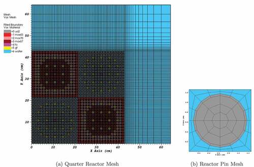
The first test problem is the well-known two-dimensional (2D) C5G7 reactor benchmark problem.²⁸ We model one quarter of the lattice, with reflecting boundary conditions on left and bottom sides, and vacuum boundary conditions on right and top sides. We use a mesh refinement that was shown to produce very small spatial discretization error, shown in Fig. 1 (Ref. 29). Multigroup cross sections are defined in the problem specification. We use discrete ordinates with a Gauss-Legendre-Chebyshev product quadrature, with 8 polar and 16 azimuthal directions per quadrant, which has been shown to be sufficient to resolve the angular discretization error to within a few pcm (Ref. 29). These problems were run on the Quartz supercomputer at Lawrence Livermore National Laboratory on six nodes and 196 concurrent processes. The problem was split into 14 processes in x by 14 processes in y. We note that this is not the optimal layout for parallelism of transport sweeps but is a better distribution for parallelism of the diffusion solution.

Fig. 1. Mesh and materials for one-quarter geometry of the C5G7 reactor benchmark.

Table I presents results for four different iterative strategies—two strategies for scattering iterations within the transport steps, with and without the use a diffusion problem for acceleration. One scattering strategy is to fully converge the scattering source during each transport step [labeled “Converged” and meaning $S_{con}=S$ and $S_{rec}=S_{lag}=0$ in Eq. (7(7) $\left({\vec{\mathrm{\Omega }}}_m\cdot \vec{\mathrm{\nabla }}+T\right){\mathrm{\Psi }}_m^{(i+1)}=\frac{1}{4\pi }\left(\begin{array}{c}{S}_{m,con}{\mathrm{\Phi }}^{(i+1)}+S_{m,rec}{\mathrm{\Phi }}^{(i+1/2)}\\ +S_{m,lag}{\mathrm{\Phi }}^{(i)}+\frac{1}{k^{(t)}}F{\mathrm{\Phi }}_0^{(t)}\end{array}\right),$(7) )]; the other is to perform a single transport sweep independently across all groups [labeled “1-Sweep” and meaning $S_{lag}=S$ and $S_{con}=S_{rec}=0$ in Eq. (7)(7) $\left({\vec{\mathrm{\Omega }}}_m\cdot \vec{\mathrm{\nabla }}+T\right){\mathrm{\Psi }}_m^{(i+1)}=\frac{1}{4\pi }\left(\begin{array}{c}{S}_{m,con}{\mathrm{\Phi }}^{(i+1)}+S_{m,rec}{\mathrm{\Phi }}^{(i+1/2)}\\ +S_{m,lag}{\mathrm{\Phi }}^{(i)}+\frac{1}{k^{(t)}}F{\mathrm{\Phi }}_0^{(t)}\end{array}\right),$(7) ]. (There are possible levels of scattering convergence between these two limits. We have not explored these in detail.) Problems that use the diffusion eigenvalue-like acceleration are labeled “k-Accel.” We compare the effect of performing the cell-by-cell DFEM update step at various points in the iteration: end of iteration (labeled “End”); after every diffusion operation (labeled “CDFEM,” since this is the original CDFEM method); and performing a no consistency step (labeled “CFEM,” as this is the same as using a CFEM basis for the diffusion problem). For this problem, we used Richardson iteration when we fully converged the within-group scattering transport problems.

TABLE I Results from 2D C5G7 Problem

Transport Scattering	Converged	Converged	1-Sweep	1-Sweep	1-Sweep	1-Sweep
Acceleration method	N/A^a	k-Accel.	N/A	k-Accel.	k-Accel.	k-Accel.
Discontinuous update	N/A	End	N/A	End	CDFEM	CFEM
Transport steps	49	6	2038	15	15	17
Sweep time (s)	8515	1187	2677	41.7	41.3	47.2
Diffusion time (s)	N/A	90.7	N/A	15.2	15.1	15.8

^aN/A = Not Applicable.

As expected, we have found that the optimal method is to perform only one transport sweep per PI. The number of transport sweeps required to converge the eigenvalue to $1.0E-7$ and the eigenvector to $1.0E-5$ without acceleration is around 2000. For this problem, a CFEM diffusion additive correction is remarkably effective, reducing the overall iteration count to 17 even when only one transport sweep is executed per iteration. Employing the one-cell discontinuous-correction updates, either after every CFEM diffusion solution or only after convergence of the CFEM diffusion PIs, does improve the correction, reducing the iteration count even further, to 15. We note that the discontinuous update step is an inexpensive operation, requiring only the independent solutions of single-cell linear systems, with the number of unknowns equaling the number of vertices in each cell.

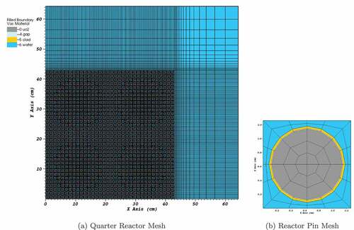
Next, we study a problem that is a modification of the C5G7 design. In this problem the spatial mesh resolves fuel, gap, guide tubes, instrumentation tubes, and cladding. We employ the Finite-Element-with-Discontiguous-Support (FEDS) energy discretization with 191 energy unknowns (including 59 in the resolved-resonance range).³⁰ We used only UO₂ assemblies to simplify cross-section generation. The mesh is illustrated in Fig. 2. The FEDS energy discretization provides increased accuracy over standard multigroup but adds upscattering in the resolved-resonance range even when scattering is physically only downscattering. This problem is meant to test the applicability of the linear DSA for eigenvalues with a more complicated scattering operator and also to test the ability of the CDFEM DSA to handle small transparent regions such as the gap between fuel and cladding.

Fig. 2. Mesh and materials for one-quarter geometry of the C5G191 reactor.

We set the eigenvalue residual tolerance to $1.0E-5$ and the eigenvector residual tolerance of the $L_2$ norm to $1.0E-5$. We use adaptive error estimates to guard against false convergence, which requires smaller relative difference between successive iterates if the observed error-reduction factor is close to 1 (Ref. 1).

The previous problem made it clear that a single transport sweep per overall iteration is the most efficient strategy, so here we test that strategy with and without DSA. Results are summarized in Table II. We observe that the within-group scattering problem is computationally expensive to converge. Iterating on only the scattering operator does not efficiently reduce the eigenvalue residual.

TABLE II Results from 2D C5G191 Problem

Transport Scattering	1-Sweep	1-Sweep
Acceleration method	N/A^a	k-Accel.
Error-reduction factor	0.991	0.743
Transport steps	852	23
Total time (h)	12.2	1.14

^aN/A = Not Applicable.

Without acceleration, the one-sweep method has an error-reduction factor near unity. This is remedied by using the diffusion eigenvalue-like problem to accelerate the solution, not only speeding convergence but also removing the issue of false convergence.

The final problem we test is a C5G7 problem in three dimensions, which we include to demonstrate that the linear DSA methodology with our chosen CDFEM low-order operator also works well in three dimensions. This is the C5G7 problem with the same mesh in the x-y plane, extruded in the third dimension according to the benchmark designation with axial meshing sufficient to accurately resolve the solution. As before, we set the eigenvalue residual tolerance to $1.0E-5$ and the eigenvector residual tolerance of the $L_2$ norm to $1.0E-5$. Results are shown in Table III. The performance of the iterative method is similar to that in two dimensions, reducing the required number of transport sweeps for $1.0E-5$ convergence to only 14. The unaccelerated method was converging so slowly that we terminated the run to avoid wasting compute cycles.

TABLE III Results from Three-Dimensional C5G7 Problem

Transport Scattering	1-Sweep	1-Sweep
Acceleration method	N/A^a	k-Accel.
Error-reduction factor	0.980	0.633
Transport steps	128^b	14
Total time (h)	24^b	2.35

^aN/A = Not Applicable.

^bTerminated without converging after 24 h of run time.

V. CONCLUSIONS

The use of diffusion operators as preconditioners of transport operators for scattering iterations has been widespread. In this paper, we consider using diffusion operators to accelerate the convergence of eigenvalue iterations. Currently, the most widely used methods to accelerate eigenvalue iterations employ nonlinear functionals in the low-order operators and solve low-order problems that are themselves standard eigenvalue problems.

Here, we have explored a family of methods, developed by Adams in 1986 and independently by Suslov in 2003, that employs a low-order eigenvalue-like problem with a fixed source to obtain an updated eigenvalue estimate and an additive correction to the eigenfunction. This method uses linear functionals and operators that were developed for scattering iterations and has demonstrated convergence rates similar to methods with nonlinear functionals.

In this paper, we have addressed several theoretical concerns regarding the multiple possible solutions that could be admitted by the eigenvalue-like problem that results from this family of methods. We have shown that the low-order linear diffusion problem becomes algebraically equivalent to the quasi-diffusion low-order problem when the solution is close to the converged solution. Through a Fourier analysis in an infinite homogeneous medium, we have shown that the iteration rapidly converges to the correct eigenvalue and eigenvector and not an arbitrary solution. We have shown that for one-cell homogeneous problems, the iteration procedure is convergent and converges to the correct eigenvalue if the high-order and low-order operators satisfy a mild consistency requirement, namely, that they produce eigenvalues that are within a factor of 2 of each other.

Finally, we add to the body of evidence that these methods work well for reactor problems, in particular, in combination with the continuous/discontinuous finite element diffusion operator we have developed. We have demonstrated that the method provides convergence of $k$ problems to $1E-5$ with only $\approx 15$ transport sweeps for the well-known C5G7 benchmarks in two dimensions and three dimensions and also for a similar problem with more spatial detail and with 191 energy unknowns.

We find the family of linear eigenvalue-like methods to be robust, rapidly convergent, and easy to implement. We emphasize that if a transport code already uses a diffusion operator (or other low-order operator) as a preconditioner to accelerate convergence of scattering iterations, it is straightforward to apply the same operator to eigenvalue acceleration, using the equations described herein, without the need to develop nonlinear functionals.

Acknowledgments

We thank Jim E. Morel and Edward W. Larsen for helpful conversations. We thank W. Daryl Hawkins for help with implementation of the method into the PDT code and with the generation of numerical results. We also thank Carolyn N. McGraw for assistance with reactor inputs and Jijie Lou for generating multigroup FEDS cross sections.

Disclosure Statement

No potential conflict of interest was reported by the author(s).

References

- M. ADAMS and E. LARSEN, “Fast Iterative Methods for Discrete-Ordinates Particle Transport Calculations,” Prog. Nucl. Energy, 40, 1, 3 (2002); https://doi.org/10.1016/S0149-1970(01)00023-3.
- H. PARK, D. A. KNOLL, and C. K. NEWMAN, “Nonlinear Acceleration of Transport Criticality Problems,” Nucl. Sci. Eng., 172, 1, 52 (2012); https://doi.org/10.13182/NSE11-81.
- K. S. SMITH, “Full-Core, 2-D, LWR Core Calculations with CASMO-4E,” Proc. PHYSOR 2002, Seoul, Korea, 2002.
- G. GUNOW, B. FORGET, and K. SMITH, “Full Core 3D Simulation of the BEAVRS Benchmark with OpenMOC,” Ann. Nucl. Energy, 134, 299 (2019); https://doi.org/10.1016/j.anucene.2019.05.050.
- L. R. CORNEJO and D. Y. ANISTRATOV, “Nonlinear Diffusion Acceleration Method with Multigrid in Energy for k-Eigenvalue Neutron Transport Problems,” Nucl. Sci. Eng., 184, 4, 514 (2016); https://doi.org/10.13182/NSE16-78.
- L. R. CORNEJO and D. Y. ANISTRATOV, “The Multilevel Quasidiffusion Method with Multigrid in Energy for Eigenvalue Transport Problems,” Prog. Nucl. Energy, 101, 401 (2017); https://doi.org/10.1016/j.pnucene.2017.05.014.
- R. E. ALCOUFFE, “Diffusion Synthetic Acceleration Methods for the Diamond-Differenced Discrete-Ordinates Equations,” Nucl. Sci. Eng., 64, 2, 344 (1977); https://doi.org/10.13182/NSE77-1.
- D. Y. ANISTRATOV and V. Y. GOL’DIN, “Multilevel Quasidiffusion Methods for Solving Multigroup Neutron Transport k-Eigenvalue Problems in One-Dimensional Slab Geometry,” Nucl. Sci. Eng., 169, 2, 111 (2011); https://doi.org/10.13182/NSE10-64.
- E. LARSEN and B. KELLEY, “CMFD and Coarse-Mesh DSA,” Proc. Int.Conf. PHYSOR 2012, Knoxville, Tennessee, April 15–20, 2012, Vol. 1, p. 728, American Nuclear Society (2012).
- K. SMITH, A. HENRY, and R. LORETZ, “The Determination of Homogenized Diffusion Theory Parameters for Coarse Mesh Nodal Analysis,” Proc. Conf. Advances Reactor Physics and Shielding, Sun Valley, Idaho, September 14–17, 1980, p. 294, American Nuclear Society (1980).
- D. A. KNOLL, H. PARK, and K. SMITH, “Application of the Jacobian-Free Newton-Krylov Method to Nonlinear Acceleration of Transport Source Iteration in Slab Geometry,” Nucl. Sci. Eng., 167, 2, 122 (2011); https://doi.org/10.13182/NSE09-75.
- M. ADAMS, “Synthetically Accelerated Heterogeneous Response-Matrix Method for Linear Transport Calculations,” PhD Thesis, University of Michigan (1986).
- M. ADAMS and E. LARSEN, “Synthetic Acceleration of One-Group SN k-Eigenvalue Problems,” Trans. Am. Nucl. Soc., 57 (1988).
- I. SUSLOV, “An Algebraic Collapsing Acceleration Method for Acceleration of the Inner (Scattering) Iterations in Long Characteristics Transport Theory,” Proc. Int. Conf. Supercomputing in Nuclear Applications, Paris, France, 2003.
- E. MASIELLO and T. ROSSI, “Improvements of the Boundary Projection Acceleration Technique Applied to the Discrete-Ordinates Transport Solver in XYZ Geometries,” Proc. Int. Conf. Mathematics and Computational Methods Applied to Nuclear Science and Engineering, Sun Valley, Idaho, May 5–9, 2013, American Nuclear Society (2013).
- Z. PRINCE, Y. WANG, and L. HARBOUR, “A Diffusion Synthetic Acceleration Approach to k-Eigenvalue Neutron Transport Using PJFNK,” Ann. Nucl. Energy, 148, 107714 (2020); https://doi.org/10.1016/j.anucene.2020.107714.
- W. H. REED, “The Effectiveness of Acceleration Techniques for Iterative Methods in Transport Theory,” Nucl. Sci. Eng., 45, 3, 245 (1971); https://doi.org/10.13182/NSE71-A19077.
- E. W. LARSEN, “Unconditionally Stable Diffusion-Synthetic Acceleration Methods for the Slab Geometry Discrete Ordinates Equations. Part I: Theory,” Nucl. Sci. Eng., 82, 1, 47 (1982); https://doi.org/10.13182/NSE82-1.
- E. W. LARSEN, “Diffusion-Synthetic Acceleration Methods for Discrete-Ordinates Problems,” Transp. Theory Stat. Phys., 13, 1–2, 107 (1984); https://doi.org/10.1080/00411458408211656.
- M. L. ADAMS and W. R. MARTIN, “Boundary Projection Acceleration: A New Approach to Synthetic Acceleration of Transport Calculations,” Nucl. Sci. Eng., 100, 3, 177 (1988); https://doi.org/10.13182/NSE100-177.
- J. S. WARSA, T. A. WAREING, and J. E. MOREL, “Krylov Iterative Methods and the Degraded Effectiveness of Diffusion Synthetic Acceleration for Multidimensional SN Calculations in Problems with Material Discontinuities,” Nucl. Sci. Eng., 147, 3, 218 (2004); https://doi.org/10.13182/NSE02-14.
- M. T. CALEF et al., “Nonlinear Krylov Acceleration Applied to a Discrete Ordinates Formulation of the k-Eigenvalue Problem,” J. Comput. Phys., 238, 188 (2013); https://doi.org/10.1016/j.jcp.2012.12.024.
- J. WILLERT, H. PARK, and D. A. KNOLL, “A Comparison of Acceleration Methods for Solving the Neutron Transport k-Eigenvalue Problem,” J. Comput. Phys., 274, 681 (2014); https://doi.org/10.1016/j.jcp.2014.06.044.
- H. G. STONE and M. L. ADAMS, “A Piecewise Linear Finite Element Basis with Application to Particle Transport,” Proc. Topl. Mtg. Nuclear Mathematical and Computational Sciences, Gatlinburg, Tennessee, April 6–11, 2003, p. 6, American Nuclear Society (2003).
- T. S. BAILEY et al., “A Piecewise Linear Finite Element Discretization of the Diffusion Equation for Arbitrary Polyhedral Grids,” J. Comput. Phys., 227, 8, 3738 (2008); https://doi.org/10.1016/j.jcp.2007.11.026.
- T. S. BAILEY, “The Piecewise Linear Discontinuous Finite Element Method Applied to the RZ and XYZ Transport Equations,” PhD Thesis, Texas A&M University (2008).
- A. P. BARBU and M. L. ADAMS, “Semi-Consistent Diffusion Synthetic Acceleration for Discontinuous Discretizations of Transport Problems,” Proc. Int. Conf. Mathematics, Computational Methods and Reactor Physics, Saratoga Springs, New York, May 3–7, 2009, American Nuclear Society (2009).
- E. LEWIS et al., “Benchmark Specification for Deterministic 2-D/3-D MOX Fuel Assembly Transport Calculations Without Spatial Homogenization (C5G7 MOX),” Organisation for Economic Co-operation and Development, Nuclear Energy Agency, Nuclear Science Committee, p. 280 (2001).
- C. N. MCGRAW et al., “Accuracy of the Linear Discontinuous Galerkin Method for Reactor Analysis with Resolved Fuel Pins,” Texas A&M University (2015).
- A. TILL, “Finite Elements with Discontiguous Support for Energy Discretization in Particle Transport,” PhD Thesis, Texas A&M University (2015).