Introduction of the Adding and Doubling Method for Solving Bateman Equations for Nuclear Fuel Depletion

Abstract

This paper introduces and evaluates the Adding and Doubling Method (ADM) for solving the Bateman equations for depletion systems with varying numbers of nuclides and compares it to the Chebyshev Rational Approximation Method (CRAM), both implemented in the reactor physics analysis application Griffin. ADM, when applied to the Crank-Nicolson Finite Difference method, can produce results comparable in accuracy and precision to CRAM with comparable run times for systems with 35 or 297 nuclides. For systems with more than 300 nuclides, the matrix-matrix operations required by ADM are significantly more costly than the matrix-vector operations required by CRAM, making CRAM the more efficient method for systems with large numbers of nuclides. ADM is an accurate method that maintains other advantages over CRAM in that it does not depend on pre-generated coefficients or require complex number operations. ADM also manages to outperform CRAM by a factor of more than 250 in terms of run time for depletion systems that require multiple Bateman solves while the depletion matrix and time step size remain constant over all depletion intervals.

Keywords:

• Adding and Doubling Method
• Bateman equation
• depletion
• Chebyshev Rational Approximation Method

I. INTRODUCTION

The Bateman equations, named after mathematician Harry Bateman, form the mathematical model describing the abundances of various nuclides in a system as time passes and radioactive decay occurs, transforming radioactive nuclides into their decay products.¹ While the Bateman equations originally considered only radioactive decay, they can be modified to account for the neutron transmutation that occurs in nuclear systems. This is shown in Eq. (1)(1) $\begin{array}{cc}\frac{d{N}_i(t)}{dt}& =\sum _j{\gamma }_{j,i}{\sigma }_{f,j}{N}_j(t)\varphi (t)+\sum _k\left(\sum _r{\sigma }_{r,k\to i}{N}_k(t)\varphi (t)\right)\\ \hspace{0.17em}& +\sum _l{\lambda }_{l\to i}{N}_l(t)-{\sigma }_{a,i}{N}_i(t)\varphi (t)-{\lambda }_i{N}_i(t)\end{array},$(1) adapted from Ref. 2:

(1) $\begin{array}{cc}\frac{d{N}_i(t)}{dt}& =\sum _j{\gamma }_{j,i}{\sigma }_{f,j}{N}_j(t)\varphi (t)+\sum _k\left(\sum _r{\sigma }_{r,k\to i}{N}_k(t)\varphi (t)\right)\\ \hspace{0.17em}& +\sum _l{\lambda }_{l\to i}{N}_l(t)-{\sigma }_{a,i}{N}_i(t)\varphi (t)-{\lambda }_i{N}_i(t)\end{array},$(1)

where

$\frac{d{N}_i(t)}{dt}$	=	= time-dependent rate of change in the number density of nuclide $i$
${\gamma }_{j,i}$ =	=	probability that nuclide $i$ will be produced as a fission product as a result of the neutron-induced nuclear fission of nuclide $j$
${\sigma }_{f,j}$ =	=	monoenergetic microscopic fission cross section of nuclide $j$
$N_j(t)$ =	=	time-dependent number density of nuclide $j$
$\varphi (t)$ =	=	time-dependent monoenergetic neutron flux within the system
${\sigma }_{r,k\to i}$ =	=	monoenergetic microscopic nonscattering, nonfission reaction cross section of reaction type $r$ of nuclide $k$, which produces nuclide $i$
$N_k(t)$ =	=	time-dependent number density of nuclide $k$
${\lambda }_{l\to i}$ =	=	decay constant of nuclide $l$, which produces nuclide $i$
$N_l(t)$ =	=	time-dependent number density of nuclide $l$
$N_i(t)$ =	=	time-dependent number density of nuclide $i$
${\sigma }_{a,i}$ =	=	monoenergetic microscopic absorption (nonscattering) cross section of nuclide $i$
${\lambda }_i$ =	=	decay constant of nuclide $i$.

When tracking systems with more than one nuclide, matrix-vector notation is convenient to describe the change in nuclide number densities:

(2) $\frac{d\mathbf{N}}{dt}=\mathbf{A}(t)\mathbf{N}(t),$(2)

where

$\mathbf{N}(t)$ =	=	time-dependent vector of the number densities of all nuclides in the system
$\frac{d\mathbf{N}}{dt}$ =	=	time-dependent vector of the rate of change of the number densities of all nuclides in the system
$\mathbf{A}(t)$ =	=	time-dependent matrix of the terms from Eq. (1)(1) $\begin{array}{cc}\frac{d{N}_i(t)}{dt}& =\sum _j{\gamma }_{j,i}{\sigma }_{f,j}{N}_j(t)\varphi (t)+\sum _k\left(\sum _r{\sigma }_{r,k\to i}{N}_k(t)\varphi (t)\right)\\ \hspace{0.17em}& +\sum _l{\lambda }_{l\to i}{N}_l(t)-{\sigma }_{a,i}{N}_i(t)\varphi (t)-{\lambda }_i{N}_i(t)\end{array},$(1) for each nuclide in the system, also known as the “depletion matrix.”

When expressed in matrix-vector notation, the number densities of all nuclides at any point in time can be determined by solving the matrix exponential, where $\mathbf{A}$ for some length of time $t$ is constant (i.e., microscopic cross sections and neutron flux are constant) and the initial number densities of all nuclides in the system ${\mathbf{N}}_0$ are known:

(3) $\mathbf{N}(t)=e^{\mathbf{A}t}{\mathbf{N}}_0.$(3)

The definition of a matrix exponential is a power series:

(4) $e^{\mathbf{A}t}=\sum _{i=0}^{\mathrm{\infty }}\frac{{(\mathbf{A}t)}^i}{i!}$(4)

Depending on the nuclides being considered, the depletion matrix can become extraordinarily stiff when considering the decay constants of long- and short-lived nuclides, such as ²⁰⁹Bi (half-life of $6.3\times {10}^{26}$ s) and ⁴H (half-life of $1.9\times {10}^{-22}$ s) that have roughly 48 orders of magnitude difference in their half-lives. While this is an extreme example, it is not uncommon to consider depletion systems where there may be a 30 or 40 order of magnitude difference between the largest and smallest terms in the depletion matrix, which presents numerical challenges for many traditional matrix exponential solvers, such as solving the power series directly.³

In this paper, we evaluate a numerical method, referred to as the Adding and Doubling Method (ADM), in order to determine how accurately and efficiently it can solve the Bateman equations when compared to one of the more prolific methods: the Chebyshev Rational Approximation Method (CRAM).

I.A. Nuclide Number Densities

Throughout this work, the unit for the number density of a nuclide is atoms per barn per centimeter $\left(\frac{\mathrm{a}\mathrm{t}\mathrm{o}\mathrm{m}\mathrm{s}}{\mathrm{b}\cdot \mathrm{c}\mathrm{m}}\right)$. This enables high-concentration nuclides in certain materials to be defined without very large or very small exponential terms. As an example, the number density of liquid water at 0℃ and atmospheric pressure is roughly $0.0335$ $\frac{\mathrm{a}\mathrm{t}\mathrm{o}\mathrm{m}\mathrm{s}}{\mathrm{b}\cdot \mathrm{c}\mathrm{m}}$ or $0.0556$ $\frac{\mathrm{m}\mathrm{o}\mathrm{l}}{\mathrm{c}{\mathrm{m}}^3}$. The reason for using number density rather than molarity is that it is computationally much easier to work with the number density directly, and microscopic neutron cross sections are expressed in units of barns, making arithmetic operations simpler:

(5) $1\frac{\mathrm{a}\mathrm{t}\mathrm{o}\mathrm{m}\mathrm{s}}{\mathrm{b}\cdot \mathrm{c}\mathrm{m}}={10}^{30}\frac{\mathrm{a}\mathrm{t}\mathrm{o}\mathrm{m}\mathrm{s}}{{\mathrm{m}}^3}={10}^{24}\frac{\mathrm{a}\mathrm{t}\mathrm{o}\mathrm{m}\mathrm{s}}{\mathrm{c}{\mathrm{m}}^3}\approx 1.66\frac{\mathrm{m}\mathrm{o}\mathrm{l}}{\mathrm{c}{\mathrm{m}}^3}.$(5)

II. CHEBYSHEV RATIONAL APPROXIMATION METHOD

This section provides a brief overview of CRAM (Refs. 4 and 5) as well as documentation of its benefits and shortcomings. CRAM was developed by Pusa and Leppänen specifically to solve Bateman equations and was first deployed in Serpent, a Monte Carlo particle transport code developed at the VTT Technical Research Center of Finland.⁶ Since then, CRAM has been deployed in other applications capable of performing depletion analyses, such as the Oak Ridge Isotope Generation and Depletion Code (ORIGEN), developed at Oak Ridge National Laboratory,⁷ and Griffin, developed at Idaho National Laboratory (INL) and Argonne National Laboratory.^8,9

CRAM relies on a min/max approximation theory applied to the scalar exponential, which leads to a partial fraction decomposition (PFD) that is a sum of $K$ rational partial fractions of order unity, where $K$ is also the polynomial degree. The approximation requires $\frac{K}{2}$ matrix inversions. The large number of required matrix inversions was one of the primary shortcomings of CRAM. Further development work on CRAM yielded two major improvements:

1. The application of sparse Gaussian elimination (SGE) to the CRAM equations resulted in the ability to avoid performing a direct matrix inversion (DMI), which enabled a significant run-time reduction for a system with 1600 nuclides while preserving numerical accuracy.¹⁰

2. The use of incomplete partial fraction (IPF) decomposition by forming a second-order rational partial fraction by combining two partial fractions, which resulted in a reduced roundoff error and the ability to perform solves at higher approximation orders.¹¹

These two improvements resulted in four different versions of CRAM that can be deployed, any of which can be referred to as “CRAM” despite their differences:

1. PFD with DMI, which was the first form of CRAM developed

2. PFD with SGE

3. IPF decomposition with DMI

4. IPF decomposition with SGE, which is the most modern version of CRAM and the version currently deployed in Serpent.

Note that each of the above versions of CRAM also requires a specified approximation order, with approximation orders for CRAM with PFD known up to Approximation Order 20 and the approximation orders for CRAM with IPF known up to Approximation Order 48 because of data limitations.

To our knowledge, CRAM with IPF and SGE is the most modern and efficient version. It benefits from the improvements of IPF over PFD, which enabled higher approximation orders and a reduced error without any increase in run time when comparing IPF and PFD at the same approximation order. It also benefits from the use of SGE over DMI, which reduced the run time by avoiding the need to perform costly matrix inversions. Consequently, for the rest of this work, when comparisons to CRAM are made or referenced (e.g., “CRAM-16”), we are referring to CRAM with IPF and SGE at the given approximation order to ensure that the most optimal version of CRAM is used and a fair comparison is made between ADM and CRAM.

Before proceeding, we highlight two primary drawbacks to CRAM. The first is that CRAM is dependent on the use of published coefficients for each approximation order, as deriving the coefficients for a given approximation order of CRAM is not trivial, which is why the coefficients were published. Since there may be errors in the published coefficients (or the coefficients may not be published to a desired level of numerical precision), this can cause issues for users working with greater than double precision. The second drawback of CRAM is its numerical inconsistency, $\mathrm{\Delta }t\to 0$, which has been documented previously.¹² However, this time inconsistency can be resolved for practical purposes by increasing the CRAM approximation order.

Based on the drawbacks of CRAM, we can consider ADM a useful method if it does not possess these drawbacks even if it does not outperform CRAM in terms of run time.

For completeness, the equations used to solve CRAM with PFD and CRAM with IPF are included here:

Partial Fraction Decomposition:

(6) $\mathbf{N}(t)={\alpha }_0{\mathbf{N}}_0+2\mathrm{R}\mathrm{e}\left(\sum _{i=1}^{k/2}{\alpha }_i{(\mathbf{A}t-{\theta }_i\mathbf{I})}^{-1}\right){\mathbf{N}}_0$(6)

Incomplete Partial Fraction:

(7) $\begin{array}{rl}& \mathbf{y}={\mathbf{N}}_0\\ & \mathrm{f}\mathrm{o}\mathrm{r}i=1,2,...,k/2\mathrm{d}\mathrm{o}\\ & \mathbf{y}=2\mathrm{R}\mathrm{e}({\alpha }_i{(\mathbf{A}t-{\theta }_i\mathbf{I})}^{-1}\mathbf{y})+\mathbf{y}\\ & \mathrm{e}\mathrm{n}\mathrm{d}\mathrm{f}\mathrm{o}\mathrm{r}\\ & \mathbf{y}={\alpha }_0\mathbf{y}\\ & \mathbf{N}(t)=\mathbf{y},& (7)\end{array}$(7)

where

$t$ =	=	length of the time step over which depletion occurs
$k$ =	=	approximation order of the CRAM solve being used
${\mathbf{N}}_0$ =	=	number densities of all nuclides at the beginning of the time step
$\mathbf{N}(t)$ =	=	time-dependent vector of the number densities of all nuclides in the system at time $t$
$\mathbf{A}$ =	=	depletion matrix, which is constant over time $t$
$\mathbf{I}$ =	=	identity matrix with the same dimensions as matrix $\mathbf{A}$
${\alpha }_i$, ${\theta }_i$, ${\alpha }_0$ =	=	constants provided in the CRAM documentation for the given approximation order $k$.

III. ADDING AND DOUBLING METHOD

This section presents ADM in detail for the Crank-Nicolson Finite Difference (CNFD) response algorithm. We consider a finite difference scheme in order to avoid explicitly evaluating the matrix exponential. We do not consider two other common finite difference schemes, forward Euler and backward Euler, because they are only first-order approximations while CNFD is a second-order approximation. Additionally, limited testing showed overall worse performance for both methods compared to CNFD, which is to be expected. While forward Euler and backward Euler are slightly faster methods than CNFD, the significant degradation in accuracy, when compared to CRAM, of both methods was considered unacceptable. Consequently, we do not discuss either method further in this work and consider CNFD only.

Two key assumptions are made for the application of CNFD to the depletion matrix. The first assumption is that $\mathbf{I}+\mathbf{A}h$ or $\mathbf{I}-\mathbf{A}h$ (where $h$ is a discrete time interval) will not have a noticeably worse condition number than $\mathbf{A}$. For the depletion matrix $\mathbf{A}$, this is typically a valid assumption as $\mathbf{A}$ has terms significantly greater than 1 because of short-lived nuclides and nuclides with very large cross sections, and terms significantly less than 1, because of long-lived nuclides and nuclides with very small cross sections. The second assumption is that $\mathrm{d}\mathrm{e}\mathrm{t}(\mathbf{I}-\mathbf{A}h)\ne 0$; thus, $\mathbf{I}-\mathbf{A}h$ is invertible. For all test cases we considered, we never encountered this issue, and thus, we assume for most real-world nuclear systems this will hold true. It is possible to define depletion systems where $\mathrm{d}\mathrm{e}\mathrm{t}(\mathbf{I}-\mathbf{A}h)=0$, but this is expected to be only for depletion matrices specifically constructed to be purely upper triangular, meaning that should $(\mathbf{A}h{)}_{ii}=1,$ a zero on the diagonal will occur resulting in the determinate of the upper triangular matrix being zero and the matrix being non-invertible. Since real-world depletion matrices encountered by analysts are not purely upper triangular, this is not expected to be a concern, and in the rare instances that $\mathbf{I}-\mathbf{A}h$ is upper triangular and $(\mathbf{A}h{)}_{ii}=1$, it is expected that since $h$ is a discrete time interval, a slightly different discrete time interval could be selected such that $(\mathbf{A}h{)}_{ii}\ne 1$ for all diagonal entries, thereby guaranteeing a nonzero determinant for upper triangular matrices and thus guaranteeing that such matrix is invertible.

III.A. Crank-Nicolson Finite Difference

In order to arrive at a CNFD response matrix, we express the matrix exponential as

(8) $e^{\mathbf{A}h}=e^{\frac{\mathbf{A}h}{2}}{\left(e^{-\frac{\mathbf{A}h}{2}}\right)}^{-1}.$(8)

Before continuing, we use a scalar $x$ such that $x=\mathbf{A}h$ (and $1=\mathbf{I}$) for the sake of simplicity and generality. Consider the following rational function, which is a Padé (1,1) approximant for the exponential:

(9) $r_{1,1}(x)=\left[1+\frac{x}{2}\right]{\left[1-\frac{x}{2}\right]}^{-1},$(9)

which (if expressed in the form of a series) is also

(10) $r_{1,1}(x)=\left[1+\frac{x}{2}\right]\sum _{i=0}^{\mathrm{\infty }}{\left[\frac{x}{2}\right]}^i.$(10)

Therefore,

(11) $r_{1,1}(x)=1+x+\frac{x^2}{2}+O(x^3).$(11)

Note that the power series of the matrix exponential has the identical representation

(12) $e^x=1+x+\frac{x^2}{2}+O(x^3).$(12)

Now, we subtract Eq. (11)(11) $r_{1,1}(x)=1+x+\frac{x^2}{2}+O(x^3).$(11) from both sides of Eq. (12)(12) $e^x=1+x+\frac{x^2}{2}+O(x^3).$(12) while using the form from Eq. (9)(9) $r_{1,1}(x)=\left[1+\frac{x}{2}\right]{\left[1-\frac{x}{2}\right]}^{-1},$(9) on the left-hand side:

(13) $e^x-\left[1+\frac{x}{2}\right]{\left[1-\frac{x}{2}\right]}^{-1}=O(x^3).$(13)

Substituting $\mathbf{A}h$ for $x$ and $\mathbf{I}$ for $1$ into Eq. (13)(13) $e^x-\left[1+\frac{x}{2}\right]{\left[1-\frac{x}{2}\right]}^{-1}=O(x^3).$(13) yields

(14) $\begin{array}{cc}{e}^{\mathbf{A}h}& =\left[\mathbf{I}+\frac{\mathbf{A}h}{2}\right]{\left[\mathbf{I}-\frac{\mathbf{A}h}{2}\right]}^{-1}+O((\mathbf{A}h{)}^3)\\ {\mathbf{P}}_{CN}(\mathbf{A}h)& =\left[\mathbf{I}+\frac{\mathbf{A}h}{2}\right]{\left[\mathbf{I}-\frac{\mathbf{A}h}{2}\right]}^{-1}\\ e^{\mathbf{A}h}-{\mathbf{P}}_{CN}(\mathbf{A}h)& =O((\mathbf{A}h{)}^3).\end{array}$(14)

Thus, ${\mathbf{P}}_{CN}(\mathbf{A}h)$ is a second-order approximation method with the consideration that order for truncation methods is asserted to be $k$ in the error term $O(h^{k+1})$, which for CNFD $k=2$.

Higher-order versions of CNFD can be derived using more terms from the power series:

(15) $\begin{array}{cc}x& =\mathbf{A}h\\ e^x& =e^{\frac{x}{2}}{\left(e^{-\frac{x}{2}}\right)}^{-1}\\ e^x& \approx \left[1+\frac{x}{2}+\frac{x^2}{8}\right]{\left[1-\frac{x}{2}+\frac{x^2}{8}\right]}^{-1}\\ e^{\mathbf{A}h}& \approx \left[\mathbf{I}+\frac{\mathbf{A}h}{2}+\frac{{(\mathbf{A}h)}^2}{8}\right]{\left[\mathbf{I}-\frac{\mathbf{A}h}{2}+\frac{{(\mathbf{A}h)}^2}{8}\right]}^{-1}.\end{array}$(15)

III.B. Evaluating a Time Step

For CNFD, $\mathbf{P}(\mathbf{A}h)$ is

(16) $P(Ah){=}^{\tilde{P}}(Ah)\left[I+O({(Ah)}^{\alpha })\right]\alpha =3.$(16)

The exact solution, denoted by $\mathbf{N}(t)$ for $2^j$ discretizations, is found by consecutive multiplication of the response matrix $\mathbf{P}$ $2^j$ number of times:

(17) $\mathbf{N}(t)=\prod _{i=1}^{2^j}\mathbf{P}(\mathbf{A}h(t,j)){\mathbf{N}}_0={\mathbf{P}}_j(\mathbf{A}h(t,j)){\mathbf{N}}_0,$(17)

where

(18) $\begin{array}{cc}{\mathbf{P}}_j(\mathbf{A}h(t,j))& ={\left[\mathbf{P}(\mathbf{A}h(t,j))\right]}^{2^j}\\ h(t,j)& =\frac{t}{2^j}.\end{array}$(18)

Equation (17)(17) $\mathbf{N}(t)=\prod _{i=1}^{2^j}\mathbf{P}(\mathbf{A}h(t,j)){\mathbf{N}}_0={\mathbf{P}}_j(\mathbf{A}h(t,j)){\mathbf{N}}_0,$(17) is equivalent to a standard finite difference solution. If, for example, $j=10$, there are $2^{10}=1024$ discretizations; that many multiplications of a large matrix, say $n=1600$, would be extremely costly for a single time $t$. Additionally, the limits of double precision result in a dramatic increase in truncation error as $j$ increases because of the large number of arithmetic operations and subsequent rounding after each operation. A more efficient method of evaluating Eq. (17)(17) $\mathbf{N}(t)=\prod _{i=1}^{2^j}\mathbf{P}(\mathbf{A}h(t,j)){\mathbf{N}}_0={\mathbf{P}}_j(\mathbf{A}h(t,j)){\mathbf{N}}_0,$(17) is necessary, which requires the principle of doubling.

One such efficient multiplication is to first determine $\mathbf{N}(t_1)$ and then at indices $2^q$ for $q=1,2,...,j$ as follows:

(19) $\begin{array}{rl}& \mathbf{N}(t_1)=\mathbf{P}(\mathbf{A}h(t,j)){\mathbf{N}}_0\\ & \mathbf{N}(t_2)=\mathbf{P}(\mathbf{A}h(t,j))\mathbf{N}(t_1)\\ & \mathbf{N}(t_2)=\left[\mathbf{P}(\mathbf{A}h(t,j))\mathbf{P}(\mathbf{A}h(t,j))\right]{\mathbf{N}}_0\\ & \mathbf{N}(t_4)=\left[\mathbf{P}(\mathbf{A}h(t,j))\mathbf{P}(\mathbf{A}h(t,j))\right]\mathbf{N}(t_2)\\ & \mathbf{N}(t_4)=\left(\left[\mathbf{P}(\mathbf{A}h(t,j))\mathbf{P}(\mathbf{A}h(t,j))\right]\right.\left.\left[\mathbf{P}(\mathbf{A}h(t,j))\mathbf{P}(\mathbf{A}h(t,j))\right]\right){\mathbf{N}}_0\\ & \mathbf{N}(t_8)=(\mathbf{P}(\mathbf{A}h(t,j)){)}^4\mathbf{N}(t_4)\\ & \mathbf{N}(t_8)=\left[{(\mathbf{P}(\mathbf{A}h(t,j)))}^4{(\mathbf{P}(\mathbf{A}h(t,j)))}^4\right]{\mathbf{N}}_0\\ & \mathbf{N}(t_{2^q})=(\mathbf{P}(\mathbf{A}h(t,j)){)}^{2^{q-1}}\mathbf{N}(t_{2^{q-1}})\\ & \mathbf{N}(t_{2^q})=\left[{(\mathbf{P}(\mathbf{A}h(t,j)))}^{2^{q-1}}{(\mathbf{P}(\mathbf{A}h(t,j)))}^{2^{q-1}}\right]{\mathbf{N}}_0\\ & \mathbf{N}(t_{2^j})=(\mathbf{P}(\mathbf{A}h(t,j)){)}^{2^{j-1}}\mathbf{N}(t_{2^{j-1}})\\ & \mathbf{N}(t_{2^j})=(\mathbf{P}(\mathbf{A}h(t,j)){)}^{2^j}{\mathbf{N}}_0.& (19)\end{array}$(19)

We call this process doubling to $t$. The advantage of doubling is that instead of requiring $2^j$ matrix-matrix multiplications, only $j$ matrix-matrix multiplications are necessary. The principle of doubling here is identical to the process used by the “scaling and squaring” method commonly used to evaluate the matrix exponential.³

Each use of ADM requires the specification of $j$ (which we refer to as the approximation power) when determining the size of the discrete subinterval $h(t,j)=\frac{t}{2^j}$. Thus, when we refer to a given solve for ADM, we may refer to it as ADM–10, which would refer to ADM with $j=10$ resulting in a discrete subinterval of length $h(t,10)=\frac{t}{2^{10}}=\frac{t}{1024}$.

We now introduce the principle of “adding,” which involves undoing some of the implementation of doubling. The final stage of doubling for a given approximation power $j$ is

(20) $({\mathbf{P}}_{j-1}(\mathbf{A}h(t,j)){)}^2{\mathbf{N}}_0={\mathbf{P}}_{j-1}(\mathbf{A}h(t,j)){\mathbf{P}}_{j-1}(\mathbf{A}h(t,j)){\mathbf{N}}_0={\mathbf{P}}_j(\mathbf{A}h(t,j)){\mathbf{N}}_0=\mathbf{N}(t).$(20)

There are two ways to solve Eq. (20)(20) $({\mathbf{P}}_{j-1}(\mathbf{A}h(t,j)){)}^2{\mathbf{N}}_0={\mathbf{P}}_{j-1}(\mathbf{A}h(t,j)){\mathbf{P}}_{j-1}(\mathbf{A}h(t,j)){\mathbf{N}}_0={\mathbf{P}}_j(\mathbf{A}h(t,j)){\mathbf{N}}_0=\mathbf{N}(t).$(20) once ${\mathbf{P}}_{j-1}(\mathbf{A}h(t,j))$ is known. A single matrix-matrix multiplication can be performed to calculate ${\mathbf{P}}_j(\mathbf{A}h(t,j))$ and then perform a matrix-vector multiplication to calculate ${\mathbf{P}}_j(\mathbf{A}h(t,j)){\mathbf{N}}_0=\mathbf{N}(t)$. Alternatively, two matrix-vector multiplications could be performed instead:

(21) ${\mathbf{P}}_{j-1}(\mathbf{A}h(t,j))({\mathbf{P}}_{j-1}(\mathbf{A}h(t,j)){\mathbf{N}}_0)=\mathbf{N}(t).$(21)

We refer to this process as adding because through the matrix-vector multiplication operations, we are effectively sequentially adding the results of two substeps together. Two matrix-vector multiplication operations are less computationally expensive than performing one matrix-matrix multiplication and one matrix-vector multiplication; thus, it is always preferable to not perform the final matrix-matrix multiplication in favor of matrix-vector multiplication. Additionally, earlier matrix-matrix multiplications could be avoided in favor of matrix-vector multiplication as follows:

(22) ${\mathbf{P}}_{j-2}(\mathbf{A}h(t,j))\left\{{\mathbf{P}}_{j-2}(\mathbf{A}h(t,j))\left[{\mathbf{P}}_{j-2}(\mathbf{A}h(t,j))({\mathbf{P}}_{j-2}(\mathbf{A}h(t,j)){\mathbf{N}}_0)\right]\right\}=\mathbf{N}(t).$(22)

Now we are replacing one matrix-matrix multiplication and two matrix-vector multiplications with four matrix-vector multiplications. We show the relationship between the number of matrix-matrix multiplications and matrix-vector operations required by ADM in Eq. (23)(23) $\begin{array}{cc}j& =m+v\\ \mathrm{M}\mathrm{M}\mathrm{M}& =m\\ \mathrm{M}\mathrm{V}\mathrm{M}& {=2}^v\end{array},$(23) :

(23) $\begin{array}{cc}j& =m+v\\ \mathrm{M}\mathrm{M}\mathrm{M}& =m\\ \mathrm{M}\mathrm{V}\mathrm{M}& {=2}^v\end{array},$(23)

where

$j$	=	= approximation power of ADM
MMM	=	= number of matrix-matrix multiplications
MVM	=	= number of matrix-vector multiplications.

When we perform the ADM comparisons, we first investigate with $m=j$, which represents “pure” doubling and no adding ($v=0$). After we have determined a suitable approximation power, we will investigate varying $m$ and $v$ values to arrive at the optimal number of matrix-matrix and matrix-vector operations or, in other words, the optimal ratio of adding to doubling.

For the remainder of this work, we will only consider applying ADM to the original CNFD method, as higher-order forms of CNFD suffer from numerical stability issues in raising the depletion matrix to a given power, which can result in the method failing because of the limits of working in double precision with a potentially stiff matrix, with failure in this instance resulting in the calculation of significantly different number densities from CRAM as well as negative number densities. Even more concerning, higher-order forms of CNFD failed for only some of the systems tested, making these higher-order forms dangerously inconsistent and thus not suitable for deployment in analysis tools that operate in double precision, such as Griffin. Hence, when we refer to ADM for the rest of this work, we are referring to ADM applied with CNFD.

III.C. Numerical Implementation of ADM and CRAM

Here we considered a simple numerical implementation of ADM and determined the length of the discrete interval $h(t,j)$ based on the approximation power ADM-$j$ specified and the length of the depletion interval $t$ specified

(24) $h(t,j)=\frac{t}{2^j}$(24)

and then solved for the initial response matrix $\mathbf{P}(\mathbf{A}h(t,j))$. Once the response matrix was calculated, we performed $j$ matrix-matrix multiplications to calculate $(\mathbf{P}(\mathbf{A}h(t,j)){)}^{2^j}$. If $j=4$, the process is

(25) $\begin{array}{rl}& (\mathbf{P}(\mathbf{A}h(t,j){)}^{2^1}=\mathbf{P}(\mathbf{A}h(t,j))\mathbf{P}(\mathbf{A}h(t,j))\\ & (\mathbf{P}(\mathbf{A}h(t,j)){)}^{2^2}=(\mathbf{P}(\mathbf{A}h(t,j)){)}^{2^1}(\mathbf{P}(\mathbf{A}h(t,j)){)}^{2^1}\\ & (\mathbf{P}(\mathbf{A}h(t,j)){)}^{2^3}=(\mathbf{P}(\mathbf{A}h(t,j)){)}^{2^2}(\mathbf{P}(\mathbf{A}h(t,j)){)}^{2^2}\\ & (\mathbf{P}(\mathbf{A}h(t,j)){)}^{2^4}=(\mathbf{P}(\mathbf{A}h(t,j)){)}^{2^3}(\mathbf{P}(\mathbf{A}h(t,j)){)}^{2^3}\\ & {\mathbf{P}}_4(\mathbf{A}h(t,j))=(\mathbf{P}(\mathbf{A}h(t,j)){)}^{2^4}\\ & h(t,j=4)=\frac{t}{2^4}=\frac{t}{16}.& (25)\end{array}$(25)

After finding the final response matrix, we performed a matrix-vector multiplication with an example for $j=4$:

(26) $\mathbf{N}(t)={\mathbf{P}}_4(\mathbf{A}h(t,4)){\mathbf{N}}_0={\mathbf{P}}_4\left(\frac{\mathbf{A}t}{16}\right){\mathbf{N}}_0.$(26)

When testing varying the number of matrix-matrix and matrix-vector multiplications, we followed the process explained in Sec. III.B.

For performing matrix-matrix and matrix-vector multiplications, we used sparse matrix multiplication routines implemented in Griffin.⁸ For performing any matrix inversions, which are needed for ADM, we used the DGETRF and DGETRI routines from LAPACK (Ref. 13). We note that the LAPACK routines are dense matrix operations, meaning that there is the potential for using an optimized sparse matrix inversion operation to reduce the cost of the matrix inversions required by ADM. However, for all practical uses of ADM, we anticipated that the matrix-matrix multiplication operations will be the more expensive part of the ADM solve.

For solving CRAM, we used the optimized SGE algorithms specified in Ref. 10, the IPF algorithm defined in Eq. (7(7) $\begin{array}{rl}& \mathbf{y}={\mathbf{N}}_0\\ & \mathrm{f}\mathrm{o}\mathrm{r}i=1,2,...,k/2\mathrm{d}\mathrm{o}\\ & \mathbf{y}=2\mathrm{R}\mathrm{e}({\alpha }_i{(\mathbf{A}t-{\theta }_i\mathbf{I})}^{-1}\mathbf{y})+\mathbf{y}\\ & \mathrm{e}\mathrm{n}\mathrm{d}\mathrm{f}\mathrm{o}\mathrm{r}\\ & \mathbf{y}={\alpha }_0\mathbf{y}\\ & \mathbf{N}(t)=\mathbf{y},& (7)\end{array}$(7) ), and sparse back-substitution, all implemented in Griffin.

IV. TEST CASES

We considered five different nuclide libraries to evaluate the performance of CRAM and ADM:

1. A 297-nuclide library from the DRAGON5 application for a beginning-of-life (BOL) pressurized water reactor (PWR) fuel pin.¹⁴

2. A 1450-nuclide library from the ORIGEN application for a BOL PWR fuel pin.⁷

3. A 1599-nuclide library that is the same as the 1450 ORIGEN library with some additional short-lived nuclides of light elements (hydrogen to aluminum) added from the Evaluated Nuclear Data File (ENDF) decay library.¹⁵ These short-lived nuclides are asserted to be produced as fission products from uranium as no other transmutation pathways existed for the nuclides to be produced.

4. A 35-nuclide library that uses nuclides tracked from an Organisation for Economic Co-operation and Development (OECD) Sodium Fast Reactor (SFR) benchmark with decay and cross-section data taken from the DRAGON5 297-nuclide library.¹⁶

5. A 693-nuclide library that uses the same library as the 1599-nuclide library but with all nuclides with decay constants greater than ${10}^{-4}$ s^–1 removed from the system and their decay chains commuted. As an example, consider the nuclide ⁴H, which has an extraordinarily short half-life. When ⁴He undergoes an $(n,p)$ reaction, instead of producing ⁴H, which then rapidly decays to ³H, we remove ⁴H from the system and assume that ³H is directly produced from ⁴He undergoing an $(n,p)$ reaction. This was done in order to generate a reduced library to serve as an intermediate between the 297- and 1450-nuclide libraries. Commuting short-lived nuclides (i.e., nuclides with large decay constants) is preferred since most nuclides of interest are either stable or have decay constants smaller than ${10}^{-4}$ s^–1.

These test cases test two libraries from applications used within the nuclear engineering field as well as a 1599-nuclide library, which closely matches the size of the libraries used for testing CRAM in its various publications, and a 35-nuclide library, which closely resembles the nuclides tracked for an extensively tested SFR benchmark problem. A 693-nuclide library serves as an intermediate size between 297 and 1450. Numerically, the smaller the depletion matrix becomes, the easier solving the Bateman equations should be since a smaller matrix requires fewer arithmetic operations. Additionally, smaller depletion matrices are expected to be less stiff since shrinking the depletion matrix often means ignoring short-lived nuclides, which are the main source of stiffness in the depletion matrix. However, when considering systems that only experience radioactive decay, small matrices may remain very stiff within a single decay chain, such as the ²³²Th and ²³⁸U decay series.

In terms of time periods, we considered depletion intervals of 1 s, 1 h (3600 s), and 1000 h ($3.6\times {10}^6$ s). All systems are treated as an infinite homogeneous region irradiated with a constant neutron flux of ${10}^{15}$ $\frac{\mathrm{n}\mathrm{e}\mathrm{u}\mathrm{t}\mathrm{r}\mathrm{o}\mathrm{n}\mathrm{s}}{\mathrm{c}{\mathrm{m}}^2\cdot \mathrm{s}}.$

In order to measure how well methods compare to one another in terms of accuracy, we considered the simple standards of maximum nuclide absolute relative difference (MNARD) and average nuclide absolute relative difference (ANARD). MNARD corresponds to the number density of a single nuclide where the magnitude of the relative difference between the number density calculated by the two methods being compared is the greatest. ANARD corresponds to the average of the absolute relative difference values of all nuclides between the two methods. Should the average and maximum differences differ significantly for a given method, then there are specific nuclides that one or both methods have difficulty accurately calculating the number density of. If both MNARD and ANARD are similar, one method has a given level of precision in comparing to another method for all nuclides considered. Last, for methods where it is relevant, we considered negative nuclide number densities (NNNDs), or the number of nuclides with number densities less than zero. These values, when they occur, are clearly nonphysical and serve as another way to determine how valid a method is for solving the Bateman equations. NNND information is included in a given table only if there were negative number densities calculated by the method. If the column is omitted from a table, no nuclides were calculated to have negative number densities. MNARD and ANARD are always provided.

Initial number densities somewhat represented a homogenized region of light water reactor UO₂ fuel with light water coolant with no cladding. The initial number densities used for each test case are shown in Table I.

TABLE I Initial Number Densities ${\mathbf{N}}_0$ for All Test Cases Representing a Homogenized PWR Fuel Pellet with Light Water Coolant

Nuclide	Density$\left(\frac{\mathrm{a}\mathrm{t}\mathrm{o}\mathrm{m}\mathrm{s}}{\mathrm{b}\cdot \mathrm{c}\mathrm{m}}\right)$	Nuclide	Density$\left(\frac{\mathrm{a}\mathrm{t}\mathrm{o}\mathrm{m}\mathrm{s}}{\mathrm{b}\cdot \mathrm{c}\mathrm{m}}\right)$
Hydrogen-1	$0.049457000000000$	Uranium-234	$8.4512220988817\times {10}^{-6}$
Oxygen-16	$0.046688131274253$	Uranium-235	$0.0010518948891610$
Oxygen-17	$1.7748234213217\times {10}^{-5}$	Uranium-238	$0.022292593642974$

V. RESULTS

We now compare CRAM to ADM. For the purposes of fair comparison, we implemented both ADM and CRAM into Griffin.⁸ The first reason for this is that Griffin is written in C++ and the original testing for CRAM was performed in Serpent, which is written in C, meaning the performance should be similar between Griffin and the published CRAM numbers derived from Serpent (barring differences in processor speed). The second reason is that both methods involve a significant number of matrix operations, and it can be difficult to accurately assess the run time in something such as MATLAB, which has heavily optimized routines that cannot be easily deployed in production codes. These heavily optimized routines can be implemented in C++ but not without significant effort.

All results were generated using a 12-core 2.70 GHz Intel Xeon E5-2697 with all calculations performed in serial. While Griffin can be run in parallel, all calculations for this work were performed in serial to remove any potential overhead from parallelization. Even running in serial, run-time fluctuations of roughly 10% appeared when running the same problem multiple times.

Since CRAM and ADM will converge, we did not provide a high-precision reference solution for the problems we considered since the odds of two disparate methods like ADM and CRAM converging to the same erroneous result is practically zero.

There are three criteria by which we compared ADM to CRAM:

1. Precision of the solution: If ADM can provide a solution of similar precision to CRAM, it, at a minimum, has value as a reference solution.

2. Run time to obtain the solution: If ADM can produce a solution in less than or equal time as CRAM, it may supplant CRAM in analysis tools because of ADM’s increased efficiency.

3. Lines of code: If ADM can function with significantly fewer lines of code than CRAM, then it is desirable because of the simplicity of implementing and maintaining the functionality.

The CRAM run time increases as the approximation order of the method increases. Similarly, the ADM run time will increase as the size of the discretization $h(t,j)=\frac{t}{2^j}$ decreases, and $j$ increases since the number of matrix-matrix multiplications will increase.

For all tests, we compared the results calculated after one depletion interval with a length of 1 s (which is the time unit used by default in Griffin) by both ADM and CRAM. We then repeated this process 100 times for each test case in order to estimate the standard deviation of the ADM and CRAM run times. Once the run time had been evaluated, we then performed ADM and CRAM solves for 1- and 1000-h depletion intervals and compared the results in order to determine how changing the size of the depletion interval impacts the solution calculated by ADM. We do not provide run-time analyses on these longer time step solves as the depletion interval length does not have an effect on ADM or CRAM run times, which was expected. The run times of the 3600- and $3.6\times {10}^6$-s depletion intervals are identical to 1.0-s depletion interval run times for similar approximation powers of ADM and similar approximation orders of CRAM.

V.A. 297-Nuclide Test Case

We first considered the 297-nuclide test case as it provides a balance between the number of nuclides and stiffness of the matrix. In general, the ADM behavior determined using the 297-nuclide test case can then determine how to improve ADM before applying it to other systems with different numbers of nuclides and different depletion matrices.

V.A.1. Testing CRAM at Different Approximation Orders

Before comparing CRAM to ADM, we first compared CRAM to itself. As the CRAM approximation order increases, the accuracy of the solution provided by CRAM increases as well. To test this, we compared various CRAM approximation orders to the CRAM-48 solution, which is the highest approximation order of CRAM available based on published coefficients.¹¹

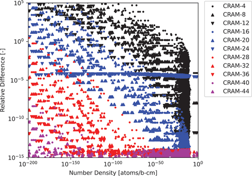
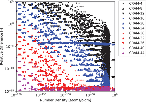
Comparisons for the 297-nuclide test case for the tested approximation orders are shown in Table II. The run times demonstrate a linear relationship between run time and increasing CRAM approximation order. The absolute relative difference between various approximation orders and Order 48 are shown in Fig. 1 with the x-axis corresponding to the number density of each nuclide as calculated by CRAM at Approximation Order 48. We drew two conclusions from Fig. 1. The first conclusion is that the comparison between Order 24 and Order 48 is markedly different from the rest of the comparisons. This is attributed to issues specifically for CRAM Order 24, which is potentially an issue with the published coefficients, since all other comparisons exhibited similar behavior. The second conclusion is that with an increasing order, the results produced by CRAM do converge with an extremely high degree of precision. This confirms that the implementation of CRAM in Griffin is performing as expected and confirms previously published results from CRAM. Finally, we considered the number of nuclides with negative number densities calculated by each CRAM approximation order shown in Table II, which clearly shows that a large number of negative values are calculated at very low approximation orders, but these disappear with an increasing order. It is also important to note that even the negative value with the greatest magnitude $\left(-3.81\times {10}^{-35}\frac{\mathrm{a}\mathrm{t}\mathrm{o}\mathrm{m}\mathrm{s}}{\mathrm{b}\cdot \mathrm{c}\mathrm{m}}\right)$ is still quite small in absolute terms, corresponding to less than one ten-thousandth of a “negative atom” per cubic meter.

TABLE II The 297-Nuclide 1.0-s Test Case Comparison of Different CRAM Approximation Orders to the CRAM-48 Solution

Order	Time (ms)	MNARD	ANARD	NNND
4	$1.190\pm 0.046$	$9.87\times {10}^7$	$3.58\times {10}^5$	38
8	$1.861\pm 0.059$	$2.65\times {10}^4$	$1.53\times {10}^2$	25
12	$2.536\pm 0.070$	$7.02\times {10}^2$	$3.18\times {10}^0$	10
16	$3.228\pm 0.094$	$4.08\times {10}^0$	$1.73\times {10}^{-2}$	1
20	$3.868\pm 0.087$	$1.16\times {10}^{-2}$	$4.70\times {10}^{-5}$	0
24	$4.534\pm 0.094$	$6.67\times {10}^{-5}$	$3.88\times {10}^{-5}$	0
28	$5.208\pm 0.106$	$2.42\times {10}^{-8}$	$9.32\times {10}^{-11}$	0
32	$5.872\pm 0.112$	$2.23\times {10}^{-11}$	$8.90\times {10}^{-14}$	0
36	$6.535\pm 0.142$	$1.46\times {10}^{-14}$	$7.32\times {10}^{-16}$	0
40	$7.175\pm 0.148$	$7.63\times {10}^{-15}$	$7.04\times {10}^{-16}$	0
44	$7.863\pm 0.145$	$9.84\times {10}^{-15}$	$2.61\times {10}^{-15}$	0
48	$8.499\pm 0.162$	—	—	0

Fig. 1. The 297-nuclide 1.0-s test case relative differences computed for various CRAM approximation orders relative to the CRAM-48 solution.

Based on the run-time results of various CRAM orders as well as the convergence of the solutions of various CRAM approximation orders as the approximation order increases, we concluded that using CRAM at Approximation Order 48 is valid for comparing to ADM. CRAM Order 48 provides the most accurate results, although its run time is roughly 33% greater than that of Order 36, which provides a comparable level of precision for the 297-nuclide test case. Consequently, should ADM, or any algorithm, slightly outperform CRAM-48 in terms of run time, comparisons between other CRAM approximation orders may be necessary.

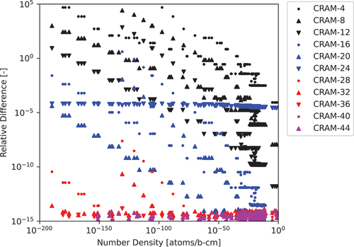
V.A.2. ADM to CRAM Comparison

We now compare ADM to the CRAM-48 solution. The first set of results for ADM are shown in Table III and Fig. 2 and indicate that with increasing approximation power, ADM converges to the CRAM-48 solution to within about 10 decimal places of accuracy as Power 20 is reached. However, Fig. 2 shows that as the approximation power increases, the relative difference between CRAM-48 and ADM increases for large number density nuclides. This trend is attributed to a compounding error from operations performed in double precision as the ADM-20 solution requires a total of one matrix inversion and 21 matrix-matrix multiplications to calculate the response matrix for the final matrix-vector operation. By contrast, while CRAM requires multiple Gaussian elimination operations, these operations do not compound upon one another in the same way as when calculating the response matrix for ADM. Also, ADM never produces any negative number densities.

TABLE III The 297-Nuclide 1.0-s Test Case Comparison of Various Approximation Powers of ADM to the CRAM-48 Solution

Power	Time (ms)	MNARD	ANARD	Power	Time (ms)	MNARD	ANARD
1	$28.102\pm 3.781$	$7.31\times {10}^4$	$3.47\times {10}^2$	11	$209.533\pm 4.456$	$5.42\times {10}^{-5}$	$1.69\times {10}^{-6}$
2	$49.388\pm 5.535$	$3.37\times {10}^2$	$2.67\times {10}^0$	12	$225.029\pm 3.715$	$1.36\times {10}^{-5}$	$4.22\times {10}^{-7}$
3	$66.955\pm 4.822$	$1.01\times {10}^1$	$1.74\times {10}^{-1}$	13	$239.717\pm 5.471$	$3.39\times {10}^{-6}$	$1.06\times {10}^{-7}$
4	$88.117\pm 6.205$	$1.18\times {10}^0$	$3.09\times {10}^{-2}$	14	$256.733\pm 6.293$	$8.48\times {10}^{-7}$	$2.64\times {10}^{-8}$
5	$106.092\pm 6.144$	$2.39\times {10}^{-1}$	$7.11\times {10}^{-3}$	15	$272.353\pm 6.443$	$2.12\times {10}^{-7}$	$6.59\times {10}^{-9}$
6	$123.549\pm 6.542$	$5.66\times {10}^{-2}$	$1.74\times {10}^{-3}$	16	$288.142\pm 7.339$	$5.30\times {10}^{-8}$	$1.65\times {10}^{-9}$
7	$142.001\pm 6.557$	$1.39\times {10}^{-2}$	$4.33\times {10}^{-4}$	17	$301.846\pm 7.313$	$1.32\times {10}^{-8}$	$4.16\times {10}^{-10}$
8	$158.481\pm 6.102$	$3.48\times {10}^{-3}$	$1.08\times {10}^{-4}$	18	$315.530\pm 7.611$	$3.31\times {10}^{-9}$	$1.10\times {10}^{-10}$
9	$172.409\pm 4.459$	$8.68\times {10}^{-4}$	$2.70\times {10}^{-5}$	19	$332.502\pm 7.635$	$8.32\times {10}^{-10}$	$4.24\times {10}^{-11}$
10	$193.101\pm 5.045$	$2.17\times {10}^{-4}$	$6.75\times {10}^{-6}$	20	$346.539\pm 8.824$	$1.75\times {10}^{-10}$	$3.71\times {10}^{-11}$

Fig. 2. The 297-nuclide 1.0-s test case relative differences computed for various ADM approximation powers to the CRAM-48 solution.

Table III reveals that the run time for ADM is greater than CRAM-48 for all approximation powers and the ADM-20 solution requires a run time 40 times greater than the CRAM run time. The main cause of this difference is the need to perform a matrix inversion coupled with several matrix-matrix multiplications while CRAM requires only matrix-vector operations. Additionally, ADM’s requirement of multiple matrix-matrix multiplications results in each subsequent matrix becoming denser, resulting in each subsequent matrix-matrix multiplication being more costly. One proposal to improve the run time of ADM-CNFD is to apply a numerical tolerance or “cutoff” to the matrices considered, treating values below this cutoff as zero whenever such a value is calculated. This reduces the number of arithmetic operations that must be performed when multiplying matrices and is expected to improve run time. From a practical perspective, we are concerned only with nuclides with number densities greater than ${10}^{-30}$ $\frac{\mathrm{a}\mathrm{t}\mathrm{o}\mathrm{m}\mathrm{s}}{\mathrm{b}\cdot \mathrm{c}\mathrm{m}}$ (or 1 $\frac{\mathrm{a}\mathrm{t}\mathrm{o}\mathrm{m}}{{\mathrm{m}}^3}$); thus, applying a cutoff is valid as long as we preserve the numerical accuracy of nuclides with number densities greater than ${10}^{-30}$ $\frac{\mathrm{a}\mathrm{t}\mathrm{o}\mathrm{m}\mathrm{s}}{\mathrm{b}\cdot \mathrm{c}\mathrm{m}}$.

We did not consider applying a numerical cutoff to CRAM as testing showed that CRAM does not significantly benefit from applying a numerical cutoff because of its matrix-vector operations. The depletion matrix, while having small values that may be zeroed, used for solving CRAM does not appreciably increase in density when performing SGE. By contrast, the matrix-matrix multiplications required by ADM can result in extraordinarily small nonzero values in the matrix, which can significantly increase the density of the ADM response matrix without those small values significantly affecting the final number density values; thus, ADM’s run time can be significantly reduced by using a numerical cutoff while CRAM does not experience a similar benefit.

Table IV shows the number of nuclides that have number densities calculated by CRAM-48 to have concentrations below the given cutoffs. Tables V through VIII as well as Fig. 3 show the impact of applying a numerical cutoff to the ADM calculation. As expected, run time improves as the numerical cutoff increases, with the ADM-20 solution with a numerical cutoff of ${10}^{-50}$ taking roughly twice as long as the CRAM-48 solution. However, MNARD and ANARD for number densities above the cutoff increased, particularly for the cutoffs of ${10}^{-100}$ and ${10}^{-50}$. Instead of considering all nuclides with number densities greater than ${10}^{-50}$ $\frac{\mathrm{a}\mathrm{t}\mathrm{o}\mathrm{m}\mathrm{s}}{\mathrm{b}\cdot \mathrm{c}\mathrm{m}}$, we specifically consider nuclides with number densities greater than ${10}^{-30}$ $\frac{\mathrm{a}\mathrm{t}\mathrm{o}\mathrm{m}\mathrm{s}}{\mathrm{b}\cdot \mathrm{c}\mathrm{m}}$ and evaluate MNARD and ANARD for these nuclides in Table IX. This indicates that a very good agreement is achieved for nuclides with number densities greater than ${10}^{-30}$ $\frac{\mathrm{a}\mathrm{t}\mathrm{o}\mathrm{m}\mathrm{s}}{\mathrm{b}\cdot \mathrm{c}\mathrm{m}}$, with 10 digits of precision achieved at Approximation Power 16 for all nuclides that exceed ${10}^{-30}$ $\frac{\mathrm{a}\mathrm{t}\mathrm{o}\mathrm{m}\mathrm{s}}{\mathrm{b}\cdot \mathrm{c}\mathrm{m}}$ while using a numerical cutoff of ${10}^{-50}$. With a run time of 14.7 ms, ADM-16 is still almost double the CRAM-48 run time. Additionally, we can estimate that each additional matrix-matrix multiplication adds roughly 0.6 ms and that the matrix inversion takes roughly 4.8 ms, which corresponds to one-third of the ADM-16 solve run-time, meaning that an optimized matrix inversion method would potentially reduce the ADM-16 run time but not make it faster than CRAM-48.

TABLE IV The 297-Nuclide 1.0-s Test Case Number of Nuclides with CRAM-48 Calculated Number Densities Below the Given Numerical Cutoffs

Cutoff	Nuclides Below Cutoff	Cutoff	Nuclides Below Cutoff
${10}^{-200}$	0	${10}^{-50}$	52
${10}^{-150}$	11	${10}^{-30}$	79
${10}^{-100}$	29	—	—

TABLE V The 297-Nuclide 1.0-s Test Case Comparison of Various Approximation Powers of ADM with a Cutoff of ${10}^{-200}$ to the CRAM-48 Solution for Nuclides with Number Densities Greater Than ${10}^{-200}$ $\frac{\mathrm{a}\mathrm{t}\mathrm{o}\mathrm{m}\mathrm{s}}{\mathrm{b}\cdot \mathrm{c}\mathrm{m}}$

Power	Time (ms)	MNARD	ANARD	Power	Time (ms)	MNARD	ANARD
1	$12.805\pm 0.585$	$7.31\times {10}^4$	$3.47\times {10}^2$	11	$71.406\pm 0.769$	$5.42\times {10}^{-5}$	$1.69\times {10}^{-6}$
2	$19.527\pm 0.295$	$3.37\times {10}^2$	$2.67\times {10}^0$	12	$76.391\pm 0.780$	$1.36\times {10}^{-5}$	$4.22\times {10}^{-7}$
3	$26.225\pm 0.453$	$1.01\times {10}^1$	$1.74\times {10}^{-1}$	13	$81.803\pm 0.893$	$3.39\times {10}^{-6}$	$1.06\times {10}^{-7}$
4	$32.257\pm 0.438$	$1.18\times {10}^0$	$3.09\times {10}^{-2}$	14	$86.383\pm 0.980$	$8.48\times {10}^{-7}$	$2.64\times {10}^{-8}$
5	$38.442\pm 0.588$	$2.39\times {10}^{-1}$	$7.11\times {10}^{-3}$	15	$91.313\pm 0.805$	$2.12\times {10}^{-7}$	$6.59\times {10}^{-9}$
6	$44.211\pm 0.509$	$5.66\times {10}^{-2}$	$1.74\times {10}^{-3}$	16	$96.251\pm 0.803$	$5.30\times {10}^{-8}$	$1.65\times {10}^{-9}$
7	$50.078\pm 0.621$	$1.39\times {10}^{-2}$	$4.33\times {10}^{-4}$	17	$102.088\pm 1.673$	$1.32\times {10}^{-8}$	$4.16\times {10}^{-10}$
8	$55.918\pm 0.650$	$3.48\times {10}^{-3}$	$1.08\times {10}^{-4}$	18	$106.656\pm 1.916$	$3.31\times {10}^{-9}$	$1.10\times {10}^{-10}$
9	$61.595\pm 0.783$	$8.68\times {10}^{-4}$	$2.70\times {10}^{-5}$	19	$109.628\pm 0.770$	$8.32\times {10}^{-10}$	$4.24\times {10}^{-11}$
10	$65.964\pm 0.636$	$2.17\times {10}^{-4}$	$6.75\times {10}^{-6}$	20	$113.387\pm 1.009$	$1.75\times {10}^{-10}$	$3.71\times {10}^{-11}$

TABLE VI The 297-Nuclide 1.0-s Test Case Comparison of Various Approximation Powers of ADM with a Cutoff of ${10}^{-150}$ to the CRAM-48 Solution for Nuclides with Number Densities Greater Than ${10}^{-150}$ $\frac{\mathrm{a}\mathrm{t}\mathrm{o}\mathrm{m}\mathrm{s}}{\mathrm{b}\cdot \mathrm{c}\mathrm{m}}$

Power	Time (ms)	MNARD	ANARD	Power	Time (ms)	MNARD	ANARD
1	$7.963\pm 0.446$	$7.31\times {10}^4$	$3.49\times {10}^2$	11	$28.045\pm 0.547$	$5.42\times {10}^{-5}$	$1.16\times {10}^{-6}$
2	$10.170\pm 0.515$	$3.37\times {10}^2$	$2.35\times {10}^0$	12	$30.439\pm 0.783$	$1.36\times {10}^{-5}$	$2.91\times {10}^{-7}$
3	$12.274\pm 0.542$	$1.01\times {10}^1$	$1.30\times {10}^{-1}$	13	$31.418\pm 0.632$	$3.39\times {10}^{-6}$	$7.28\times {10}^{-8}$
4	$14.815\pm 0.541$	$1.18\times {10}^0$	$2.17\times {10}^{-2}$	14	$33.176\pm 0.699$	$8.48\times {10}^{-7}$	$1.82\times {10}^{-8}$
5	$16.672\pm 0.467$	$2.39\times {10}^{-1}$	$4.93\times {10}^{-3}$	15	$35.028\pm 0.695$	$2.12\times {10}^{-7}$	$4.55\times {10}^{-9}$
6	$18.972\pm 0.572$	$5.66\times {10}^{-2}$	$1.20\times {10}^{-3}$	16	$36.596\pm 0.746$	$5.30\times {10}^{-8}$	$1.14\times {10}^{-9}$
7	$20.752\pm 0.572$	$1.39\times {10}^{-2}$	$2.99\times {10}^{-4}$	17	$38.026\pm 0.614$	$1.32\times {10}^{-8}$	$2.88\times {10}^{-10}$
8	$22.644\pm 0.487$	$3.48\times {10}^{-3}$	$7.46\times {10}^{-5}$	18	$39.563\pm 0.746$	$3.31\times {10}^{-9}$	$7.75\times {10}^{-11}$
9	$24.624\pm 0.726$	$8.68\times {10}^{-4}$	$1.86\times {10}^{-5}$	19	$40.754\pm 0.856$	$8.32\times {10}^{-10}$	$3.45\times {10}^{-11}$
10	$26.567\pm 0.805$	$2.17\times {10}^{-4}$	$4.66\times {10}^{-6}$	20	$42.389\pm 0.779$	$1.75\times {10}^{-10}$	$3.50\times {10}^{-11}$

TABLE VII The 297-Nuclide 1.0-s Test Case Comparison of Various Approximation Powers of ADM with a Cutoff of ${10}^{-100}$ to the CRAM-48 Solution for Nuclides with Number Densities Greater Than ${10}^{-100}$ $\frac{\mathrm{a}\mathrm{t}\mathrm{o}\mathrm{m}\mathrm{s}}{\mathrm{b}\cdot \mathrm{c}\mathrm{m}}$

Power	Time (ms)	MNARD	ANARD	Power	Time (ms)	MNARD	ANARD
1	$6.978\pm 0.517$	$4.18\times {10}^2$	$2.53\times {10}^0$	11	$20.694\pm 0.558$	$1.87\times {10}^{-5}$	$3.30\times {10}^{-7}$
2	$8.526\pm 0.505$	$1.58\times {10}^1$	$1.56\times {10}^{-1}$	12	$21.761\pm 0.615$	$3.96\times {10}^{-6}$	$7.98\times {10}^{-8}$
3	$10.050\pm 0.486$	$1.79\times {10}^0$	$2.53\times {10}^{-2}$	13	$23.058\pm 0.593$	$8.94\times {10}^{-7}$	$1.73\times {10}^{-8}$
4	$11.446\pm 0.513$	$3.51\times {10}^{-1}$	$5.67\times {10}^{-3}$	14	$23.872\pm 0.630$	$6.46\times {10}^{-7}$	$6.46\times {10}^{-9}$
5	$12.638\pm 0.434$	$8.23\times {10}^{-2}$	$1.38\times {10}^{-3}$	15	$25.324\pm 0.781$	$8.77\times {10}^{-7}$	$4.27\times {10}^{-9}$
6	$14.070\pm 0.512$	$2.03\times {10}^{-2}$	$3.42\times {10}^{-4}$	16	$26.250\pm 0.733$	$9.34\times {10}^{-7}$	$3.74\times {10}^{-9}$
7	$15.633\pm 0.698$	$5.04\times {10}^{-3}$	$8.54\times {10}^{-5}$	17	$27.248\pm 0.575$	$9.49\times {10}^{-7}$	$3.61\times {10}^{-9}$
8	$16.615\pm 0.518$	$1.26\times {10}^{-3}$	$2.13\times {10}^{-5}$	18	$28.295\pm 0.593$	$9.52\times {10}^{-7}$	$3.59\times {10}^{-9}$
9	$17.862\pm 0.385$	$3.14\times {10}^{-4}$	$5.33\times {10}^{-6}$	19	$29.581\pm 0.598$	$9.53\times {10}^{-7}$	$3.59\times {10}^{-9}$
10	$19.169\pm 0.496$	$7.77\times {10}^{-5}$	$1.33\times {10}^{-6}$	20	$30.271\pm 0.666$	$9.53\times {10}^{-7}$	$3.60\times {10}^{-9}$

TABLE VIII The 297-Nuclide 1.0-s Test Case Comparison of Various Approximation Powers of ADM with a Cutoff of ${10}^{-50}$ to the CRAM-48 Solution for Nuclides with Number Densities Greater Than ${10}^{-50}$ $\frac{\mathrm{a}\mathrm{t}\mathrm{o}\mathrm{m}\mathrm{s}}{\mathrm{b}\cdot \mathrm{c}\mathrm{m}}$

Power	Time (ms)	MNARD	ANARD	Power	Time (ms)	MNARD	ANARD
1	$5.484\pm 0.194$	$3.22\times {10}^0$	$5.31\times {10}^{-2}$	11	$12.470\pm 0.492$	$9.74\times {10}^{-4}$	$4.48\times {10}^{-6}$
2	$6.201\pm 0.192$	$6.70\times {10}^{-1}$	$1.20\times {10}^{-2}$	12	$12.636\pm 0.323$	$9.76\times {10}^{-4}$	$4.48\times {10}^{-6}$
3	$7.005\pm 0.247$	$1.58\times {10}^{-1}$	$2.89\times {10}^{-3}$	13	$13.283\pm 0.418$	$9.77\times {10}^{-4}$	$4.47\times {10}^{-6}$
4	$7.777\pm 0.375$	$3.91\times {10}^{-2}$	$7.14\times {10}^{-4}$	14	$13.839\pm 0.435$	$9.77\times {10}^{-4}$	$4.48\times {10}^{-6}$
5	$8.972\pm 0.420$	$9.73\times {10}^{-3}$	$1.75\times {10}^{-4}$	15	$14.390\pm 0.436$	$9.77\times {10}^{-4}$	$4.48\times {10}^{-6}$
6	$8.941\pm 0.196$	$2.41\times {10}^{-3}$	$4.07\times {10}^{-5}$	16	$14.734\pm 0.246$	$9.77\times {10}^{-4}$	$4.48\times {10}^{-6}$
7	$9.594\pm 0.199$	$5.79\times {10}^{-4}$	$1.01\times {10}^{-5}$	17	$15.396\pm 0.415$	$9.77\times {10}^{-4}$	$4.48\times {10}^{-6}$
8	$10.632\pm 0.443$	$8.27\times {10}^{-4}$	$5.67\times {10}^{-6}$	18	$16.131\pm 0.468$	$9.77\times {10}^{-4}$	$4.48\times {10}^{-6}$
9	$11.033\pm 0.428$	$9.39\times {10}^{-4}$	$4.58\times {10}^{-6}$	19	$16.359\pm 0.452$	$9.77\times {10}^{-4}$	$4.48\times {10}^{-6}$
10	$11.380\pm 0.208$	$9.67\times {10}^{-4}$	$4.49\times {10}^{-6}$	20	$16.888\pm 0.402$	$9.77\times {10}^{-4}$	$4.48\times {10}^{-6}$

TABLE IX The 297-Nuclide 1.0-s Test Case Comparison of Various Approximation Powers of ADM with a Cutoff of ${10}^{-50}$ to the CRAM-48 Solution for Nuclides with Number Densities Greater Than ${10}^{-30}$ $\frac{\mathrm{a}\mathrm{t}\mathrm{o}\mathrm{m}\mathrm{s}}{\mathrm{b}\cdot \mathrm{c}\mathrm{m}}$

Power	MNARD	ANARD	Power	MNARD	ANARD
1	$1.25\times {10}^{-1}$	$2.68\times {10}^{-3}$	11	$1.19\times {10}^{-7}$	$2.56\times {10}^{-9}$
2	$3.13\times {10}^{-2}$	$6.71\times {10}^{-4}$	12	$2.98\times {10}^{-8}$	$6.40\times {10}^{-10}$
3	$7.81\times {10}^{-3}$	$1.68\times {10}^{-4}$	13	$7.45\times {10}^{-9}$	$1.60\times {10}^{-10}$
4	$1.95\times {10}^{-3}$	$4.19\times {10}^{-5}$	14	$1.86\times {10}^{-9}$	$4.06\times {10}^{-11}$
5	$4.88\times {10}^{-4}$	$1.05\times {10}^{-5}$	15	$4.66\times {10}^{-10}$	$1.10\times {10}^{-11}$
6	$1.22\times {10}^{-4}$	$2.62\times {10}^{-6}$	16	$1.19\times {10}^{-10}$	$5.37\times {10}^{-12}$
7	$3.05\times {10}^{-5}$	$6.55\times {10}^{-7}$	17	$3.31\times {10}^{-11}$	$4.68\times {10}^{-12}$
8	$7.63\times {10}^{-6}$	$1.64\times {10}^{-7}$	18	$2.07\times {10}^{-11}$	$8.39\times {10}^{-12}$
9	$1.91\times {10}^{-6}$	$4.09\times {10}^{-8}$	19	$4.91\times {10}^{-11}$	$2.01\times {10}^{-11}$
10	$4.77\times {10}^{-7}$	$1.02\times {10}^{-8}$	20	$9.44\times {10}^{-11}$	$3.45\times {10}^{-11}$

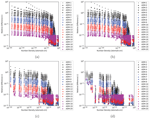
Fig. 3. The 297-nuclide 1.0-s test case relative differences computed for various ADM approximation powers with various cutoffs to the CRAM-48 solution: (a) cutoff of ${10}^{-200}$, (b) cutoff of ${10}^{-150}$, (c) cutoff of ${10}^{-100}$, and (d) cutoff of ${10}^{-50}$.

We did not consider numerical cutoffs above ${10}^{-50}$ since we see an impact on number densities that are greater than but still close to the cutoff meaning that applying a cutoff of ${10}^{-30}$ or even ${10}^{-40}$ could impact the results of number densities with concentrations greater than ${10}^{-30}$ $\frac{\mathrm{a}\mathrm{t}\mathrm{o}\mathrm{m}\mathrm{s}}{\mathrm{b}\cdot \mathrm{c}\mathrm{m}}$. For all other test cases, we used a cutoff of ${10}^{-50}$ in order to benefit from the decreased run time of ADM with said cutoff.

We now attempted to optimize the ratio of adding and doubling by varying the number of matrix-matrix operations $m$ and matrix-vector operations $2^v$. Results are shown in Table X. We achieved a minimum run time of 11.4 ms for $v=6$. This is now roughly 33% greater than the run time of CRAM-48. Changing $m$ and $v$ results in the same ADM solution, although, as $m\to 0$, the number of matrix-vector operations can introduce a loss of precision because of the large number of resulting arithmetic operations (reflected in the significant increase in run time when $m=0$).

TABLE X The 297-Nuclide 1.0-s Test Case Run-Time Comparisons for ADM-16 with a Cutoff of ${10}^{-50}$ with Varying $m$ and $v$ Numbers

$m$	$v$	Time (ms)	$m$	$v$	Time (ms)
16	0	$14.734\pm 0.246$	7	9	$15.471\pm 0.300$
15	1	$13.989\pm 0.273$	6	10	$21.639\pm 0.384$
14	2	$13.329\pm 0.297$	5	11	$34.539\pm 0.570$
13	3	$12.677\pm 0.289$	4	12	$60.035\pm 0.894$
12	4	$12.083\pm 0.239$	3	13	$111.901\pm 1.042$
11	5	$11.569\pm 0.195$	2	14	$215.705\pm 1.624$
10	6	$11.405\pm 0.257$	1	15	$419.896\pm 4.308$
9	7	$11.788\pm 0.389$	0	16	$832.604\pm 3.376$
8	8	$12.754\pm 0.255$	—	—	—

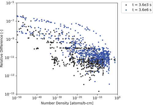
Now that we have identified the optimal conditions for ADM in terms of precision and run time for the 1-s depletion case, we consider ADM-16 applied to the 297-nuclide test case for a depletion period of 3600 s (1 h) and $3.6\times {10}^6$ s (1000 h). The main motivation for testing longer depletion intervals is twofold. First, depletion intervals for normal reactor operation are generally on the order of hours or days, with short depletion periods generally restricted to specific short-term transient modeling. Second, ADM relies on increasing its accuracy by reducing the substep size for calculating the response matrix since $O((Ah{)}^3)\to 0$ as $h\to 0,$ where $h=\frac{t}{2^j}$. As the time step length $t$ increases, the time discretization $h$ for a given ADM approximation power $j$ increases, which results in a decrease in precision.

The results of ADM-16 compared to CRAM-48 for the 297-nuclide test case for 3600 and $3.6\times {10}^6$ s are shown in Fig. 4 and Table XI. For the 3600-s depletion interval, there were 255 nuclides with number densities above ${10}^{-50}$ $\frac{\mathrm{a}\mathrm{t}\mathrm{o}\mathrm{m}\mathrm{s}}{\mathrm{b}\cdot \mathrm{c}\mathrm{m}}$ and 240 nuclides with number densities above ${10}^{-30}$ $\frac{\mathrm{a}\mathrm{t}\mathrm{o}\mathrm{m}\mathrm{s}}{\mathrm{b}\cdot \mathrm{c}\mathrm{m}}$. For the $3.6\times {10}^6$-s depletion interval, there were 268 nuclides with number densities above ${10}^{-50}$ $\frac{\mathrm{a}\mathrm{t}\mathrm{o}\mathrm{m}\mathrm{s}}{\mathrm{b}\cdot \mathrm{c}\mathrm{m}}$ and 258 nuclides with number densities above ${10}^{-30}$ $\frac{\mathrm{a}\mathrm{t}\mathrm{o}\mathrm{m}\mathrm{s}}{\mathrm{b}\cdot \mathrm{c}\mathrm{m}}$. As expected, there is a reduction in the precision of the ADM-16 solution as the length of the depletion interval increases, which means that for longer depletion intervals, it may be necessary to increase the approximation power of ADM in order to maintain the desired precision.

TABLE XI The 297-Nuclide 3600- and $3.6\times {10}^6$-s Test Case Comparison of ADM-16 with a Cutoff of ${10}^{-50}$ to the CRAM-48 Solution for Nuclides with Number Densities Greater Than ${10}^{-30}$ $\frac{\mathrm{a}\mathrm{t}\mathrm{o}\mathrm{m}\mathrm{s}}{\mathrm{b}\cdot \mathrm{c}\mathrm{m}}$

Depletion Interval (s)	MNARD	ANARD
3600	$2.32\times {10}^{-9}$	$5.92\times {10}^{-11}$
$3.6\times {10}^6$	$4.00\times {10}^{-8}$	$7.03\times {10}^{-10}$

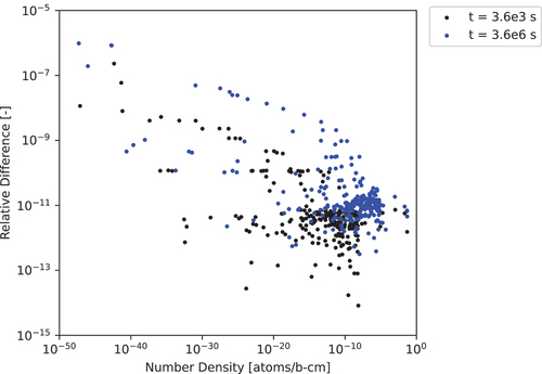
Fig. 4. The 297-nuclide 3600- and $3.6\times {10}^6$-s test case relative differences computed for ADM-16 with a cutoff of ${10}^{-50}$ to the CRAM-48 solution.

V.B. 1450-Nuclide Test Case

Now we considered a 1450-nuclide test case, which is based on a combined one-group cross-section and decay library for a BOL PWR fuel assembly from ORIGEN (Ref. 7).

V.B.1. Testing CRAM at Different Approximation Orders

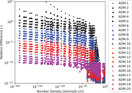
First we checked all CRAM approximation orders against the CRAM-48 solution. The results are shown in Fig. 5 and Table XII. The behavior overall appears similar to the 297-nuclide case with the caveats that convergence is slower with an increasing order and that the number of approximation orders that produce negative number densities is larger. Additionally, we see that negative number densities are calculated by all approximation orders up to 28. This once again highlights the need to use a higher CRAM approximation order to ensure that physical number densities are calculated.

TABLE XII The 1450-Nuclide 1.0-s Test Case Comparison of Various Approximation Orders of CRAM to the CRAM-48 Solution

Order	Time (ms)	MNARD	ANARD	NNND
4	$7.695\pm 0.323$	$2.56\times {10}^{18}$	$3.97\times {10}^{15}$	210
8	$10.976\pm 0.423$	$2.27\times {10}^{11}$	$1.23\times {10}^9$	149
12	$14.567\pm 0.402$	$4.74\times {10}^8$	$7.84\times {10}^5$	144
16	$17.897\pm 0.453$	$6.53\times {10}^6$	$1.73\times {10}^4$	104
20	$21.283\pm 0.524$	$9.32\times {10}^4$	$2.26\times {10}^2$	50
24	$25.081\pm 0.741$	$6.82\times {10}^2$	$1.54\times {10}^0$	19
28	$28.018\pm 0.576$	$3.00\times {10}^0$	$6.41\times {10}^{-3}$	2
32	$31.366\pm 0.687$	$8.82\times {10}^{-3}$	$1.80\times {10}^{-5}$	0
36	$35.200\pm 0.780$	$1.88\times {10}^{-5}$	$3.70\times {10}^{-8}$	0
40	$38.106\pm 0.668$	$3.08\times {10}^{-8}$	$5.87\times {10}^{-11}$	0
44	$41.362\pm 0.692$	$4.04\times {10}^{-11}$	$7.64\times {10}^{-14}$	0
48	$44.983\pm 0.630$	—	—	0

Fig. 5. The 1450-nuclide 1.0-s test case relative differences computed for various CRAM approximation orders to the CRAM-48 solution.

V.B.2. ADM to CRAM Comparison

We then compared ADM to the CRAM-48 result for the 1450-nuclide case using a ${10}^{-50}$ cutoff to maintain accuracy for nuclides with number densities greater than ${10}^{-30}$ $\frac{\mathrm{a}\mathrm{t}\mathrm{o}\mathrm{m}\mathrm{s}}{\mathrm{b}\cdot \mathrm{c}\mathrm{m}}$. See Fig. 6 and Table XIII. As determined by the CRAM-48 solution, 1165 nuclides have number densities above ${10}^{-50}$ $\frac{\mathrm{a}\mathrm{t}\mathrm{o}\mathrm{m}\mathrm{s}}{\mathrm{b}\cdot \mathrm{c}\mathrm{m}}$, and 1026 nuclides have number densities greater than ${10}^{-30}$ $\frac{\mathrm{a}\mathrm{t}\mathrm{o}\mathrm{m}\mathrm{s}}{\mathrm{b}\cdot \mathrm{c}\mathrm{m}}$. A 10-digit agreement is achieved at Approximation Power 17 with a run time over four times as long as CRAM-48. Each additional matrix-matrix multiplication adds roughly 7.3 ms to the ADM run time, and the matrix inversion takes roughly 80 ms, once again about one-third of the ADM-17 run time.

TABLE XIII The 1450-Nuclide 1.0-s Test Case Comparison of Various Approximation Powers of ADM with a Cutoff of ${10}^{-50}$ to the CRAM-48 Solution for Nuclides with Number Densities Greater Than ${10}^{-30}$ $\frac{\mathrm{a}\mathrm{t}\mathrm{o}\mathrm{m}\mathrm{s}}{\mathrm{b}\cdot \mathrm{c}\mathrm{m}}$

Power	Time (ms)	MNARD	ANARD	Power	Time (ms)	MNARD	ANARD
1	$87.527\pm 3.245$	$1.26\times {10}^0$	$1.69\times {10}^{-2}$	11	$171.336\pm 1.837$	$1.06\times {10}^{-6}$	$1.14\times {10}^{-8}$
2	$97.568\pm 1.499$	$2.88\times {10}^{-1}$	$3.37\times {10}^{-3}$	12	$177.757\pm 2.024$	$2.65\times {10}^{-7}$	$2.84\times {10}^{-9}$
3	$106.814\pm 1.122$	$7.02\times {10}^{-2}$	$7.47\times {10}^{-4}$	13	$184.864\pm 1.944$	$6.64\times {10}^{-8}$	$7.11\times {10}^{-10}$
4	$115.902\pm 1.174$	$1.74\times {10}^{-2}$	$1.86\times {10}^{-4}$	14	$191.530\pm 2.048$	$1.66\times {10}^{-8}$	$1.78\times {10}^{-10}$
5	$124.660\pm 1.493$	$4.35\times {10}^{-3}$	$4.66\times {10}^{-5}$	15	$197.297\pm 1.780$	$4.15\times {10}^{-9}$	$4.47\times {10}^{-11}$
6	$133.319\pm 1.476$	$1.09\times {10}^{-3}$	$1.17\times {10}^{-5}$	16	$203.416\pm 1.711$	$1.04\times {10}^{-9}$	$1.28\times {10}^{-11}$
7	$141.832\pm 2.368$	$2.72\times {10}^{-4}$	$2.91\times {10}^{-6}$	17	$209.008\pm 1.493$	$2.59\times {10}^{-10}$	$6.58\times {10}^{-12}$
8	$148.941\pm 1.506$	$6.79\times {10}^{-5}$	$7.29\times {10}^{-7}$	18	$214.349\pm 1.892$	$6.84\times {10}^{-11}$	$9.06\times {10}^{-12}$
9	$156.760\pm 1.196$	$1.70\times {10}^{-5}$	$1.82\times {10}^{-7}$	19	$222.910\pm 6.465$	$6.40\times {10}^{-11}$	$1.64\times {10}^{-11}$
10	$163.923\pm 1.588$	$4.25\times {10}^{-6}$	$4.55\times {10}^{-8}$	20	$225.825\pm 1.937$	$1.30\times {10}^{-10}$	$3.25\times {10}^{-11}$

Fig. 6. The 1450-nuclide 1.0-s test case relative differences computed for various ADM approximation powers with a cutoff of ${10}^{-50}$ to the CRAM-48 solution.

We then evaluated ADM-17 for varying $m$ and $v$ values. As shown in Table XIV, a run-time improvement is initially seen with an increasing $v$ until $v=7$, at which point run time degrades as the number of matrix-vector multiplications reaches into the thousands, while precision for nuclides with densities greater than ${10}^{-30}$ $\frac{\mathrm{a}\mathrm{t}\mathrm{o}\mathrm{m}\mathrm{s}}{\mathrm{b}\cdot \mathrm{c}\mathrm{m}}$ is consistent. This is a similar $v$ value that resulted in a maximum run-time improvement for the 297-nuclide test case. Even with the run-time improvement, ADM-17 is still roughly three times slower than CRAM-48. Based on these results and the 297-nuclide test case results, it appears that ADM performs worse than CRAM with an increasing matrix size.

TABLE XIV The 1450-Nuclide 1.0-s Run-Time Comparisons of Various $m$ and $v$ Values for ADM-17 with a Cutoff of ${10}^{-50}$

$m$	$v$	Time (ms)	$m$	$v$	Time (ms)
17	0	$209.008\pm 1.493$	8	9	$187.608\pm 1.666$
16	1	$195.543\pm 1.462$	7	10	$239.931\pm 1.727$
15	2	$185.906\pm 2.944$	6	11	$351.685\pm 1.954$
14	3	$176.691\pm 1.550$	5	12	$577.568\pm 2.041$
13	4	$168.687\pm 2.010$	4	13	$1028.398\pm 2.842$
12	5	$161.333\pm 1.298$	3	14	$1925.427\pm 4.519$
11	6	$156.377\pm 1.274$	2	15	$3688.520\pm 33.674$
10	7	$156.375\pm 1.264$	1	16	$7122.559\pm 142.493$
9	8	$167.378\pm 3.972$	0	17	$14333.752\pm 290.456$

Now we once again consider the 3600- and $3.6\times {10}^6$-s depletion interval test cases for ADM-17 compared to CRAM-48.

The results of this comparison are shown in Fig. 7 and Table XV. For the 3600-s depletion interval, there were 1260 nuclides with number densities above ${10}^{-50}$ $\frac{\mathrm{a}\mathrm{t}\mathrm{o}\mathrm{m}\mathrm{s}}{\mathrm{b}\cdot \mathrm{c}\mathrm{m}}$ and 1112 nuclides with number densities above ${10}^{-30}$ $\frac{\mathrm{a}\mathrm{t}\mathrm{o}\mathrm{m}\mathrm{s}}{\mathrm{b}\cdot \mathrm{c}\mathrm{m}}$. For the $3.6\times {10}^6$-s depletion interval, there were 1367 nuclides with number densities above ${10}^{-50}$ $\frac{\mathrm{a}\mathrm{t}\mathrm{o}\mathrm{m}\mathrm{s}}{\mathrm{b}\cdot \mathrm{c}\mathrm{m}}$ and 1284 nuclides with number densities above ${10}^{-30}$ $\frac{\mathrm{a}\mathrm{t}\mathrm{o}\mathrm{m}\mathrm{s}}{\mathrm{b}\cdot \mathrm{c}\mathrm{m}}$. Once again, there is a reduction in precision as the length of the depletion interval increases, but the decrease in precision is more severe for certain nuclides in the $3.6\times {10}^6$ s. In this case, the maximum difference between ADM and CRAM solutions occurred for ⁸Be, which is a very short-lived nuclide. A short-lived nuclide should be the most difficult to calculate because of the stiffness it introduces into the depletion matrix, and that is reflected here.

TABLE XV The 1450-Nuclide 3600- and $3.6\times {10}^6$-s Test Case Comparison of ADM-17 with a Cutoff of ${10}^{-50}$ to the CRAM-48 Solution for Nuclides with Number Densities Greater Than ${10}^{-30}$ $\frac{\mathrm{a}\mathrm{t}\mathrm{o}\mathrm{m}\mathrm{s}}{\mathrm{b}\cdot \mathrm{c}\mathrm{m}}$

Depletion Interval (s)	MNARD	ANARD
3600	$3.21\times {10}^{-9}$	$1.91\times {10}^{-11}$
$3.6\times {10}^6$	$3.38\times {10}^{-6}$	$2.61\times {10}^{-9}$

Fig. 7. The 1450-nuclide 3600- and $3.6\times {10}^6$-s test case relative differences computed for ADM-17 with a cutoff of ${10}^{-50}$ to the CRAM-48 solution.

V.C. 1599-Nuclide Test Case

We now considered a 1599-nuclide library, which is the same as the 1450-nuclide library except for the addition of 149 short-lived light nuclides. Because there are no decay or transmutation production pathways to these nuclides in the 1450-nuclide library, all of the added short-lived light nuclides are produced as fission products from ²³⁵U with a yield fraction of ${10}^{-7}$.

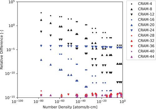
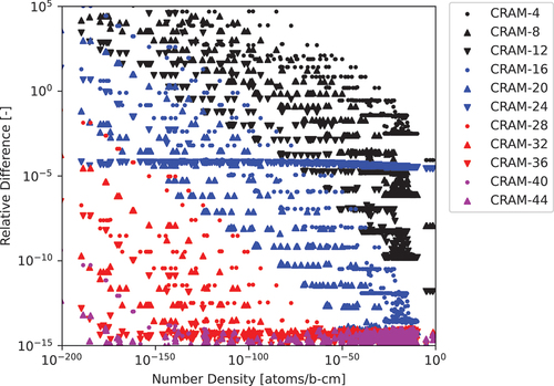
V.C.1. CRAM at Different Approximation Orders

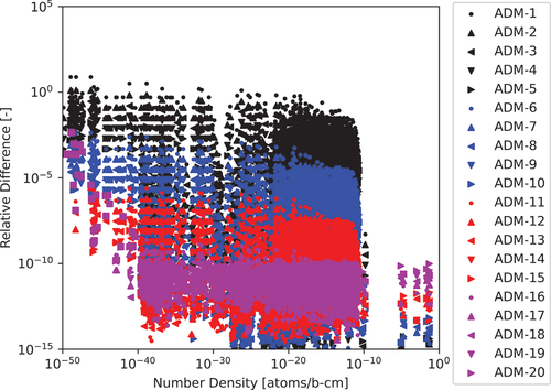
Once again, we compared the results of various CRAM approximation orders to the CRAM-48 solution. The results are shown in Table XVI and Fig. 8 and largely replicate the results from the 1450-nuclide test case. Interestingly, fewer nuclides have negative number densities for the 1599-nuclide test case compared to the 1450-nuclide test case. This implies that even if the values for specific transmutation pathways are not altered, simply adding more nuclides to the system may improve the behavior of CRAM. However, further investigation of this CRAM behavior is beyond the scope of this work.

TABLE XVI The 1599-Nuclide 1.0-s Test Case Comparison of Various Approximation Orders of CRAM to the CRAM-48 Solution

Order	Time (ms)	MNARD	ANARD	NNND
4	$8.482\pm 0.382$	$2.56\times {10}^{18}$	$3.60\times {10}^{15}$	193
8	$11.862\pm 0.359$	$2.27\times {10}^{11}$	$1.11\times {10}^9$	137
12	$15.419\pm 0.441$	$4.74\times {10}^8$	$7.07\times {10}^5$	119
16	$18.678\pm 0.468$	$6.53\times {10}^6$	$1.56\times {10}^4$	88
20	$22.072\pm 0.498$	$9.32\times {10}^4$	$2.04\times {10}^2$	43
24	$25.574\pm 0.593$	$6.82\times {10}^2$	$1.39\times {10}^0$	18
28	$29.179\pm 0.511$	$3.00\times {10}^0$	$5.80\times {10}^{-3}$	2
32	$32.891\pm 0.603$	$8.82\times {10}^{-3}$	$1.63\times {10}^{-5}$	0
36	$36.080\pm 0.751$	$1.88\times {10}^{-5}$	$3.35\times {10}^{-8}$	0
40	$39.386\pm 0.714$	$3.08\times {10}^{-8}$	$5.32\times {10}^{-11}$	0
44	$42.699\pm 0.778$	$4.04\times {10}^{-11}$	$6.92\times {10}^{-14}$	0
48	$46.326\pm 0.759$	—	—	0

Fig. 8. The 1599-nuclide 1.0-s test case relative differences computed for various CRAM approximation orders to the CRAM-48 solution.

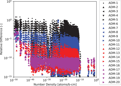
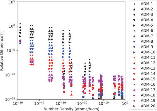
V.C.2. ADM to CRAM Comparison

We now considered ADM at various approximation powers and using a cutoff of ${10}^{-50}$ for the 1599-nuclide 1.0-s test case. 1338 nuclides have number densities above ${10}^{-50}$ $\frac{\mathrm{a}\mathrm{t}\mathrm{o}\mathrm{m}\mathrm{s}}{\mathrm{b}\cdot \mathrm{c}\mathrm{m}}$, and 1200 nuclides have number densities above ${10}^{-30}$ $\frac{\mathrm{a}\mathrm{t}\mathrm{o}\mathrm{m}\mathrm{s}}{\mathrm{b}\cdot \mathrm{c}\mathrm{m}}$. See Fig. 9 and Table XVII.

TABLE XVII The 1599-Nuclide 1.0-s Test Case Comparison of Various Approximation Powers of ADM with a Cutoff of ${10}^{-50}$ to the CRAM-48 Solution for Nuclides with Number Densities Greater Than ${10}^{-30}$ $\frac{\mathrm{a}\mathrm{t}\mathrm{o}\mathrm{m}\mathrm{s}}{\mathrm{b}\cdot \mathrm{c}\mathrm{m}}$

Power	Time (ms)	MNARD	ANARD	Power	Time (ms)	MNARD	ANARD
1	$106.663\pm 7.069$	$1.26\times {10}^0$	$8.39\times {10}^{-2}$	11	$200.935\pm 6.343$	$1.28\times {10}^{-2}$	$1.07\times {10}^{-5}$
2	$117.649\pm 7.568$	$1.00\times {10}^0$	$5.75\times {10}^{-2}$	12	$209.311\pm 6.492$	$2.65\times {10}^{-7}$	$2.69\times {10}^{-9}$
3	$127.183\pm 5.396$	$1.00\times {10}^0$	$3.78\times {10}^{-2}$	13	$215.783\pm 6.615$	$6.64\times {10}^{-8}$	$6.66\times {10}^{-10}$
4	$138.153\pm 6.418$	$1.00\times {10}^0$	$1.53\times {10}^{-2}$	14	$224.172\pm 6.700$	$1.66\times {10}^{-8}$	$1.67\times {10}^{-10}$
5	$149.537\pm 7.497$	$9.99\times {10}^{-1}$	$1.63\times {10}^{-3}$	15	$231.779\pm 7.775$	$4.15\times {10}^{-9}$	$4.20\times {10}^{-11}$
6	$158.449\pm 7.637$	$9.96\times {10}^{-1}$	$8.40\times {10}^{-4}$	16	$238.346\pm 6.112$	$1.04\times {10}^{-9}$	$1.21\times {10}^{-11}$
7	$168.013\pm 6.623$	$9.83\times {10}^{-1}$	$8.21\times {10}^{-4}$	17	$244.053\pm 6.819$	$2.59\times {10}^{-10}$	$6.39\times {10}^{-12}$
8	$177.483\pm 7.421$	$9.34\times {10}^{-1}$	$7.79\times {10}^{-4}$	18	$249.185\pm 5.953$	$6.84\times {10}^{-11}$	$9.03\times {10}^{-12}$
9	$184.055\pm 6.217$	$7.62\times {10}^{-1}$	$6.34\times {10}^{-4}$	19	$256.358\pm 6.934$	$6.40\times {10}^{-11}$	$1.68\times {10}^{-11}$
10	$192.735\pm 6.577$	$3.36\times {10}^{-1}$	$2.80\times {10}^{-4}$	20	$262.023\pm 5.549$	$1.30\times {10}^{-10}$	$3.27\times {10}^{-11}$

Fig. 9. The 1599-nuclide 1.0-s test case relative differences computed for various ADM approximation powers with a cutoff of ${10}^{-50}$ to the CRAM-48 solution.

ADM-17 provides the desired 10 digits of precision with a five times greater run time than the CRAM-48 run time. Each additional matrix-matrix multiplication adds roughly 8.2 ms to the ADM run time, and the matrix inversion takes roughly 98 ms, slightly less than one-third of the ADM-17 run time. We evaluated changing $m$ and $v$, as shown in Table XVIII. Once again, $v=7$ achieves the lowest possible run time, which is still almost four times larger than the run time for CRAM-48.

TABLE XVIII The 1599-Nuclide 1.0-s Test Case Run-Time Comparisons for Various $m$ and $v$ Values for ADM-17 with a Cutoff of ${10}^{-50}$

$m$	$v$	Time (ms)	$m$	$v$	Time (ms)
17	0	$244.053\pm 6.819$	8	9	$204.485\pm 1.116$
16	1	$234.120\pm 12.414$	7	10	$258.295\pm 2.988$
15	2	$212.482\pm 6.629$	6	11	$367.385\pm 0.949$
14	3	$198.908\pm 1.089$	5	12	$593.511\pm 3.287$
13	4	$188.696\pm 1.460$	4	13	$1044.161\pm 2.669$
12	5	$181.396\pm 2.622$	3	14	$1956.950\pm 58.433$
11	6	$176.521\pm 2.888$	2	15	$3704.073\pm 14.029$
10	7	$175.256\pm 2.989$	1	16	$7180.476\pm 138.903$
9	8	$182.397\pm 3.520$	0	17	$13952.969\pm 137.753$

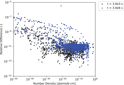
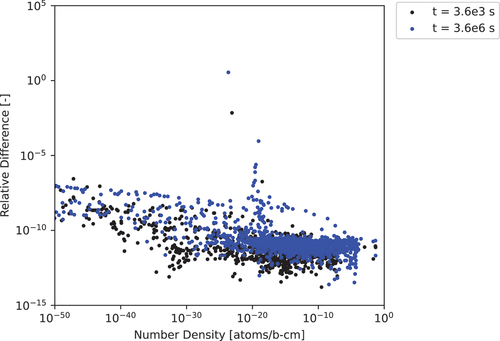
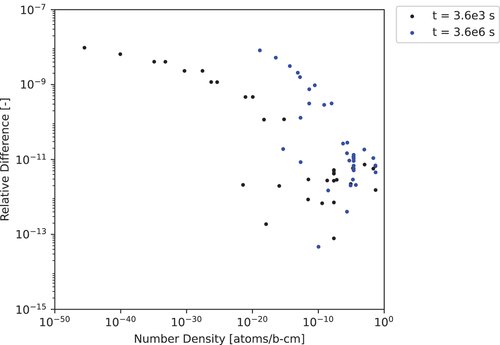
Again we considered longer time steps for the 1599-nuclide test case, with results for ADM-17 shown in Fig. 10 and Table XIX. For the 3600-s time step, there are 1432 nuclides with number densities greater than ${10}^{-50}$ $\frac{\mathrm{a}\mathrm{t}\mathrm{o}\mathrm{m}\mathrm{s}}{\mathrm{b}\cdot \mathrm{c}\mathrm{m}}$ and 1287 nuclides with number densities greater than ${10}^{-30}$ $\frac{\mathrm{a}\mathrm{t}\mathrm{o}\mathrm{m}\mathrm{s}}{\mathrm{b}\cdot \mathrm{c}\mathrm{m}}$. For the $3.6\times {10}^6$-s time step, there are 1548 nuclides with number densities greater than ${10}^{-50}$ $\frac{\mathrm{a}\mathrm{t}\mathrm{o}\mathrm{m}\mathrm{s}}{\mathrm{b}\cdot \mathrm{c}\mathrm{m}}$ and 1457 nuclides with number densities greater than ${10}^{-30}$ $\frac{\mathrm{a}\mathrm{t}\mathrm{o}\mathrm{m}\mathrm{s}}{\mathrm{b}\cdot \mathrm{c}\mathrm{m}}$. As expected, we saw a deterioration in precision across the board except for a select few nuclides, which have results incredibly diverged from the CRAM-48 solution. The largest difference corresponds to ³³Ne, a very short-lived nuclide, which should be difficult to model. Additionally, for the $3.6\times {10}^6$-s case, the ³³Ne number density calculated by ADM-17 is negative, the first and only negative number density calculated by ADM.

TABLE XIX The 1599-Nuclide 3600- and $3.6\times {10}^6$-s Test Case Comparison of ADM-17 with a Cutoff of ${10}^{-50}$ to the CRAM-48 Solution for Nuclides with Number Densities Greater Than ${10}^{-30}$ $\frac{\mathrm{a}\mathrm{t}\mathrm{o}\mathrm{m}\mathrm{s}}{\mathrm{b}\cdot \mathrm{c}\mathrm{m}}$

Depletion Interval (s)	MNARD	ANARD	NNND
3600	$0.00704$	$4.92\times {10}^{-6}$	0
$3.6\times {10}^6$	$3.53$	$0.00228$	1

Fig. 10. The 1599-nuclide 3600- and $3.6\times {10}^6$-s test case relative differences computed for ADM-17 with a cutoff of ${10}^{-50}$ to the CRAM-48 solution.

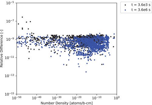
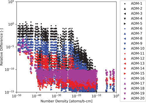
Since we observed an unacceptable divergence from CRAM-48 in the ADM-17 results, we raised the approximation power of ADM to 25 to see if convergence can be achieved as expected. Results are shown in Fig. 11 and Table XX and demonstrate the expected behavior as the maximum and average differences between ADM and CRAM decrease to acceptable levels with the increase in approximation power. This indicates that ADM-17 was not an adequate approximation power for the time step considered for the 1599-nuclide case.

TABLE XX The 1599-Nuclide 3600- and $3.6\times {10}^6$-s Comparison of ADM-25 with a Cutoff of ${10}^{-50}$ to the CRAM-48 Solution for Nuclides with Number Densities Greater Than ${10}^{-30}$ $\frac{\mathrm{a}\mathrm{t}\mathrm{o}\mathrm{m}\mathrm{s}}{\mathrm{b}\cdot \mathrm{c}\mathrm{m}}$

Depletion Interval (s)	MNARD	ANARD
3600	$3.63\times {10}^{-9}$	$1.31\times {10}^{-9}$
$3.6\times {10}^6$	$4.55\times {10}^{-9}$	$5.14\times {10}^{-10}$

Fig. 11. The 1599-nuclide 3600- and $3.6\times {10}^6$-s test case relative differences computed for ADM-25 with a cutoff of ${10}^{-50}$ to the CRAM-48 solution.

V.D. 35-Nuclide Test Case

Since with an increasing number of nuclides the performance gap between ADM and CRAM increases, we considered a smaller test case for 35 nuclides taken from an OECD SFR benchmark report to see if ADM can outperform CRAM when the number of nuclides decreases.

V.D.1. Testing CRAM at Various Approximation Orders

We compared the various approximation orders of CRAM to the CRAM-48 solution for the 1-s depletion interval. Results are shown in Fig. 12 and Table XXI with the results reflecting previously observed behavior.

TABLE XXI The 35-Nuclide 1.0-s Test Case Comparison of Various CRAM Approximation Orders to the CRAM-48 Solution

Order	Time (ms)	MNARD	ANARD	NNND
4	$0.051\pm 0.006$	$5.19\times {10}^2$	$2.49\times {10}^1$	9
8	$0.076\pm 0.007$	$1.68\times {10}^1$	$6.36\times {10}^{-1}$	2
12	$0.106\pm 0.020$	$5.75\times {10}^{-2}$	$1.99\times {10}^{-3}$	0
16	$0.126\pm 0.012$	$8.56\times {10}^{-5}$	$2.82\times {10}^{-6}$	0
20	$0.154\pm 0.013$	$7.76\times {10}^{-8}$	$2.48\times {10}^{-9}$	0
24	$0.174\pm 0.012$	$6.20\times {10}^{-5}$	$3.93\times {10}^{-5}$	0
28	$0.193\pm 0.012$	$2.55\times {10}^{-14}$	$2.14\times {10}^{-15}$	0
32	$0.229\pm 0.014$	$9.48\times {10}^{-15}$	$4.20\times {10}^{-15}$	0
36	$0.248\pm 0.015$	$5.54\times {10}^{-15}$	$1.11\times {10}^{-15}$	0
40	$0.268\pm 0.022$	$4.36\times {10}^{-15}$	$6.65\times {10}^{-16}$	0
44	$0.301\pm 0.020$	$9.48\times {10}^{-15}$	$2.01\times {10}^{-15}$	0
48	$0.317\pm 0.018$	—	—	0

Fig. 12. The 35-nuclide 1.0-s test case relative differences computed for various CRAM approximation orders relative to the CRAM-48 solution.

V.D.2. ADM to CRAM Comparison

Once again, we compared various ADM approximation powers with a cutoff of ${10}^{-50}$ to the CRAM-48 solution for the 1-s depletion interval with the results shown in Fig. 13 and Table XXII. As calculated by CRAM-48, 30 nuclides had number densities above ${10}^{-50}$ $\frac{\mathrm{a}\mathrm{t}\mathrm{o}\mathrm{m}\mathrm{s}}{\mathrm{b}\cdot \mathrm{c}\mathrm{m}}$, and 25 nuclides had number densities above ${10}^{-30}$ $\frac{\mathrm{a}\mathrm{t}\mathrm{o}\mathrm{m}\mathrm{s}}{\mathrm{b}\cdot \mathrm{c}\mathrm{m}}$. Each additional matrix-matrix multiplication adds roughly 0.014 ms to the ADM run time, and the matrix inversion takes roughly 0.047 ms, about one-fifth of the ADM-16 run time.

TABLE XXII The 35-Nuclide 1.0-s Test Case Comparisons for Various Approximation Powers of ADM with a Cutoff of ${10}^{-50}$ to the CRAM-48 Solution for Nuclides with Number Densities Greater Than ${10}^{-30}$ $\frac{\mathrm{a}\mathrm{t}\mathrm{o}\mathrm{m}\mathrm{s}}{\mathrm{b}\cdot \mathrm{c}\mathrm{m}}$

Power	Time (ms)	MNARD	ANARD	Power	Time (ms)	MNARD	ANARD
1	$0.061\pm 0.011$	$1.25\times {10}^{-1}$	$1.00\times {10}^{-2}$	11	$0.197\pm 0.015$	$1.19\times {10}^{-7}$	$9.54\times {10}^{-9}$
2	$0.078\pm 0.008$	$3.13\times {10}^{-2}$	$2.50\times {10}^{-3}$	12	$0.209\pm 0.013$	$2.98\times {10}^{-8}$	$2.38\times {10}^{-9}$
3	$0.087\pm 0.008$	$7.81\times {10}^{-3}$	$6.25\times {10}^{-4}$	13	$0.222\pm 0.017$	$7.45\times {10}^{-9}$	$5.96\times {10}^{-10}$
4	$0.106\pm 0.013$	$1.95\times {10}^{-3}$	$1.56\times {10}^{-4}$	14	$0.241\pm 0.020$	$1.86\times {10}^{-9}$	$1.50\times {10}^{-10}$
5	$0.118\pm 0.013$	$4.88\times {10}^{-4}$	$3.91\times {10}^{-5}$	15	$0.250\pm 0.015$	$4.65\times {10}^{-10}$	$3.82\times {10}^{-11}$
6	$0.129\pm 0.012$	$1.22\times {10}^{-4}$	$9.77\times {10}^{-6}$	16	$0.263\pm 0.018$	$1.19\times {10}^{-10}$	$1.22\times {10}^{-11}$
7	$0.140\pm 0.011$	$3.05\times {10}^{-5}$	$2.44\times {10}^{-6}$	17	$0.275\pm 0.014$	$3.27\times {10}^{-11}$	$7.22\times {10}^{-12}$
8	$0.155\pm 0.013$	$7.63\times {10}^{-6}$	$6.10\times {10}^{-7}$	18	$0.290\pm 0.021$	$2.00\times {10}^{-11}$	$9.76\times {10}^{-12}$
9	$0.167\pm 0.012$	$1.91\times {10}^{-6}$	$1.53\times {10}^{-7}$	19	$0.303\pm 0.019$	$4.86\times {10}^{-11}$	$1.90\times {10}^{-11}$
10	$0.187\pm 0.012$	$4.77\times {10}^{-7}$	$3.81\times {10}^{-8}$	20	$0.320\pm 0.023$	$8.70\times {10}^{-11}$	$3.72\times {10}^{-11}$

Fig. 13. The 35-nuclide 1.0-s test case relative differences computed for various ADM approximation powers with a cutoff of ${10}^{-50}$ to the CRAM-48 solution.

A 10-digit agreement is achieved with ADM-16, and the run time of 0.263 ms is less than the CRAM-48 run time of 0.317 ms. However, CRAM-28 also achieves a 14-digit agreement with CRAM-48 and requires only 0.193 ms, outperforming ADM-16. Next we considered varying $m$ and $v$ for ADM-16 with the results shown in Table XXIII. Varying $m$ and $v$ results in an optimal value of $v=5$ and reduces the run time of ADM-16 to 0.211 ms, still slightly more than CRAM-28.

TABLE XXIII The 35-Nuclide 1.0-s Test Case Run-Time Comparisons of Various m and $v$ Values for ADM-16 with a Cutoff of 10⁻⁵⁰ with Varying m and v Numbers

$m$	$v$	Time (ms)	$m$	$v$	Time (ms)
16	0	$0.263\pm 0.018$	7	9	$0.434\pm 0.032$
15	1	$0.272\pm 0.022$	6	10	$0.699\pm 0.034$
14	2	$0.245\pm 0.021$	5	11	$1.247\pm 0.058$
13	3	$0.234\pm 0.019$	4	12	$2.343\pm 0.076$
12	4	$0.223\pm 0.021$	3	13	$4.581\pm 0.150$
11	5	$0.211\pm 0.012$	2	14	$8.994\pm 0.360$
10	6	$0.218\pm 0.015$	1	15	$17.400\pm 0.312$
9	7	$0.240\pm 0.016$	0	16	$32.036\pm 0.489$
8	8	$0.298\pm 0.019$	—	—	—

Next we considered the comparison between ADM-16 with a cutoff of ${10}^{-50}$ to the CRAM-48 solution for the 3600- and $3.6\times {10}^6$-s depletion intervals. For the 3600-s depletion interval, CRAM-48 calculated that 30 nuclides had number densities greater than ${10}^{-30}$ $\frac{\mathrm{a}\mathrm{t}\mathrm{o}\mathrm{m}\mathrm{s}}{\mathrm{b}\cdot \mathrm{c}\mathrm{m}}$ and 35 nuclides had number densities greater than ${10}^{-50}$ $\frac{\mathrm{a}\mathrm{t}\mathrm{o}\mathrm{m}\mathrm{s}}{\mathrm{b}\cdot \mathrm{c}\mathrm{m}}$. For the $3.6\times {10}^6$-s depletion interval, CRAM-48 calculated that all 35 nuclides had number densities greater than ${10}^{-30}$ $\frac{\mathrm{a}\mathrm{t}\mathrm{o}\mathrm{m}\mathrm{s}}{\mathrm{b}\cdot \mathrm{c}\mathrm{m}}$. The results are shown in Fig. 14 and Table XXIV. Contrary to previous results, we see an expected degradation in precision for the 3600-s depletion interval, but the degradation does not increase for the $3.6\times {10}^6$-s depletion interval with precision improving slightly compared to the 3600-s depletion interval. This is attributed to the depletion matrix being significantly less stiff as the shortest-lived nuclide tracked is ²⁴²Am with a decay constant of $1.2\times {10}^{-5}$ s^–1, and the neutron transmutation terms are smaller in magnitude since powerful neutron absorbers such as ¹³⁵Xe and ¹⁰B are not tracked in the system. The less stiff the depletion matrix is, the more precise ADM is expected to be for longer depletion intervals. Consequently, the 3600- and $3.6\times {10}^6$-s depletion interval results have a nearly identical level of precision.

TABLE XXIV The 35-Nuclide 3600- and $3.6\times {10}^6$-s Test Case Comparison of ADM-16 with a Cutoff of ${10}^{-50}$ to the CRAM-48 Solution for Nuclides with Number Densities Greater Than ${10}^{-30}\frac{\mathrm{a}\mathrm{t}\mathrm{o}\mathrm{m}\mathrm{s}}{\mathrm{b}\cdot \mathrm{c}\mathrm{m}}$

Depletion Interval [s]	MNARD	ANARD
3,600	$9.64\times {10}^{-9}$	$9.27\times {10}^{-10}$
$3.6\times {10}^6$	$8.18\times {10}^{-9}$	$6.62\times {10}^{-10}$

Fig. 14. The 35-nuclide 3600- and $3.6\times {10}^6$-s test case relative differences computed for ADM-16 with a cutoff of ${10}^{-50}$ to the CRAM-48 solution.

V.E. 693-Nuclide Test Case

For completeness, we last considered a 693-nuclide test case in order to better understand the increasing ADM and CRAM run times as the number of nuclides increases. The library is generated using the 1599-nuclide library and applying a decay constant cutoff of ${10}^{-4}$ s^–1, where nuclides with decay constants greater than this cutoff are removed from the library. Any instances where such a nuclide would be produced via transmutation or decay instead results in the production of the decay daughters of the removed nuclide.

V.E.1. Testing CRAM at Various Approximation Orders

We compared the various approximation orders of CRAM to the CRAM-48 solution, with the results shown in Fig. 15 and Table XXV. The behavior is expected based on the results of the previous test cases considered for the other libraries.

TABLE XXV The 693-Nuclide 1.0-s Test Case Comparison of Various CRAM Approximation Orders to the CRAM-48 Solution

Order	Time (ms)	MNARD	ANARD	NNND
4	3.203 ± 0.154	1.14 × 10^15	3.27 × 10^12	122
8	5.048 ± 0.196	4.60 × 10^10	9.88 × 10^7	106
12	6.795 ± 0.280	8.06 × 10^6	2.94 × 10^4	75
16	8.702 ± 0.323	3.92 × 10^5	9.80 × 10^2	29
20	10.414 ± 0.324	4.10 × 10^3	9.47 × 10^0	13
24	12.360 ± 0.279	2.27 × 10^1	4.92 × 10^–2	3
28	13.956 ± 0.376	7.71 × 10^–2	1.60 × 10^–4	0
32	15.745 ± 0.310	1.80 × 10^–4	3.59 × 10^–7	0
36	17.429 ± 0.348	3.11 × 10^–7	6.00 × 10^–10	0
40	19.490 ± 0.444	4.19 × 10^–10	7.89 × 10^–13	0
44	20.636 ± 0.329	4.66 × 10^–13	2.06 × 10^–15	0
48	21.151 ± 0.269	—	—	0

Fig. 15. The 693-nuclide 1.0-s test case relative differences computed for various CRAM approximation orders to the CRAM-48 solution.

V.E.2. ADM to CRAM Comparison

We observed that ADM-16 achieves 10 digits of agreement with CRAM-48 with a run time that is roughly three times greater. See Fig. 16 and Table XXVI. Each additional matrix-matrix multiplication adds roughly 2.2 ms to the ADM run time, and the matrix inversion takes roughly 23 ms, about one-third of the ADM-16 run time. Varying $v$ results in the optimal decrease in run time occurring at $v=6$ with a run time roughly double the CRAM-48 solution as shown in Table XXVII.

TABLE XXVI The 693-Nuclide 1.0-s Test Case Comparison of Various Approximation Powers of ADM with a Cutoff of ${10}^{-50}$ to the CRAM-48 Solution for Nuclides with Number Densities Greater Than ${10}^{-30}$ $\frac{\mathrm{a}\mathrm{t}\mathrm{o}\mathrm{m}\mathrm{s}}{\mathrm{b}\cdot \mathrm{c}\mathrm{m}}$

Power	Time (ms)	MNARD	ANARD	Power	Time (ms)	MNARD	ANARD
1	24.981 ± 1.129	$1.25\times {10}^{-1}$	1.94 × 10^–3	11	$50.984\pm 1.917$	1.19 × 10^–7	$1.85\times {10}^{-9}$
2	27.879 ± 1.182	$3.13\times {10}^{-2}$	4.86 × 10^–4	12	$52.586\pm 1.563$	2.98 × 10^–8	$4.63\times {10}^{-10}$
3	30.591 ± 1.325	$7.81\times {10}^{-3}$	1.21 × 10^–4	13	$56.029\pm 2.324$	7.45 × 10^–9	$1.16\times {10}^{-10}$
4	33.356 ± 1.729	$1.95\times {10}^{-3}$	3.03 × 10^–5	14	$56.882\pm 1.786$	1.86 × 10^–9	$2.94\times {10}^{-11}$
5	37.009 ± 2.186	$4.88\times {10}^{-4}$	7.59 × 10^–6	15	$58.338\pm 1.297$	4.66 × 10^–10	$8.15\times {10}^{-12}$
6	39.350 ± 2.037	$1.22\times {10}^{-4}$	1.90 × 10^–6	16	$60.555\pm 1.836$	1.17 × 10^–10	$3.82\times {10}^{-12}$
7	41.469 ± 1.609	$3.05\times {10}^{-5}$	4.74 × 10^–7	17	$62.926\pm 2.174$	3.08 × 10^–11	$4.06\times {10}^{-12}$
8	44.338 ± 2.290	$7.63\times {10}^{-6}$	1.19 × 10^–7	18	$64.077\pm 1.540$	2.42 × 10^–11	$8.01\times {10}^{-12}$
9	45.645 ± 1.003	$1.91\times {10}^{-6}$	2.96 × 10^–8	19	$66.941\pm 2.232$	3.83 × 10^–11	$1.51\times {10}^{-11}$
10	49.492 ± 2.171	$4.77\times {10}^{-7}$	7.41 × 10^–9	20	$67.366\pm 1.362$	9.61 × 10^–11	$3.32\times {10}^{-11}$

TABLE XXVII The 693-Nuclide 1.0-s Test Case Run-Time Comparisons for Various $m$ and $v$ Values for ADM-16 with a Cutoff of 10⁻⁵⁰

$m$	$v$	Time (ms)	$m$	$v$	Time (ms)
16	0	$60.555\pm 1.836$	7	9	57.013 ± 0.923
15	1	$56.369\pm 1.110$	6	10	76.021 ± 0.762
14	2	$53.203\pm 0.732$	5	11	115.709 ± 1.302
13	3	$50.530\pm 0.831$	4	12	196.419 ± 1.969
12	4	$48.084\pm 0.691$	3	13	355.936 ± 3.382
11	5	$46.024\pm 0.650$	2	14	674.263 ± 2.653
10	6	$45.036\pm 0.585$	1	15	1312.431 ± 3.271
9	7	$45.171\pm 0.808$	0	16	2521.742 ± 6.839
8	8	$48.311\pm 0.734$	—	—	—

Fig. 16. The 693-nuclide 1.0-s test case relative differences computed for various ADM approximation powers with a cutoff of ${10}^{-50}$ to the CRAM-48 solution.

Again we considered the comparison between ADM-16 with a cutoff of ${10}^{-50}$ to the CRAM-48 solution for the 3600- and $3.6\times {10}^6$-s depletion intervals. For the 3600-s depletion interval, CRAM-48 calculated that 475 nuclides had number densities greater than ${10}^{-30}$ $\frac{\mathrm{a}\mathrm{t}\mathrm{o}\mathrm{m}\mathrm{s}}{\mathrm{b}\cdot \mathrm{c}\mathrm{m}}$ and 565 nuclides had number densities greater than ${10}^{-50}$ $\frac{\mathrm{a}\mathrm{t}\mathrm{o}\mathrm{m}\mathrm{s}}{\mathrm{b}\cdot \mathrm{c}\mathrm{m}}$. For the $3.6\times {10}^6$-s depletion interval, CRAM-48 calculated that 590 nuclides had number densities greater than ${10}^{-30}$ $\frac{\mathrm{a}\mathrm{t}\mathrm{o}\mathrm{m}\mathrm{s}}{\mathrm{b}\cdot \mathrm{c}\mathrm{m}}$ and 652 nuclide had number densities greater than ${10}^{-50}$ $\frac{\mathrm{a}\mathrm{t}\mathrm{o}\mathrm{m}\mathrm{s}}{\mathrm{b}\cdot \mathrm{c}\mathrm{m}}$. The results are shown in Fig. 17 and Table XXVIII and once again demonstrate the loss of precision for ADM with an increasing time step length.

TABLE XXVIII The 693-Nuclide 3600- and $3.6\times {10}^6$-s Test Case Comparison of ADM-16 with a Cutoff of ${10}^{-50}$ to the CRAM-48 Solution for Nuclides with Number Densities Greater Than ${10}^{-30}\frac{\mathrm{a}\mathrm{t}\mathrm{o}\mathrm{m}\mathrm{s}}{\mathrm{b}\cdot \mathrm{c}\mathrm{m}}$

Depletion Interval [s]	MNARD	ANARD
3,600	$6.45\times {10}^{-9}$	$9.71\times {10}^{-11}$
$3.6\times {10}^6$	$5.55\times {10}^{-8}$	$1.15\times {10}^{-9}$

Fig. 17. The 693-nuclide 3600- and $3.6\times {10}^6$-s test case relative differences computed for ADM-16 with a cutoff of ${10}^{-50}$ to the CRAM-48 solution.

V.F. Time-Independent Depletion Matrix with Fixed Depletion Step Size

So far, we have considered solving the Bateman equations under the assumption that $\mathbf{A}$ or $t$ may change from one depletion interval to the next, as shown for two hypothetical depletion intervals with lengths of $t_1$ and $t_2$:

(27) $\begin{array}{cc}\mathbf{A}(t_1)& \ne \mathbf{A}(t_2)\\ t_1& \ne t_2.\end{array}$(27)

For most reactor analysis applications, this is necessary as after each depletion interval, the change in nuclide number densities will result in the macroscopic cross sections of the materials in the reactor changing, which will consequently result in the flux profile of the reactor changing. If effects such as temperature are also being considered, the microscopic cross sections themselves will change because of Doppler broadening. All of these effects combined result in the depletion matrix $\mathbf{A}$ being time dependent for most analyses, as follows:

(28) $\begin{array}{cc}\mathbf{A}(t)& =\mathbf{D}+\mathbf{T}(t)\\ \mathbf{T}(t)& =\sum _{g=0}^G\left(\sum _{r=0}^R{\sigma }_{g,r}(t)\right){\varphi }_g(t)\end{array},$(28)

where

$t$ =	=	length of the time step over which depletion is occurring
$\mathbf{A}(t)$ =	=	time-dependent depletion matrix
$\mathbf{D}$ =	=	time-independent decay matrix
$\mathbf{T}(t)$ =	=	time-dependent neutron transmutation matrix
$G$ =	=	number of neutron energy groups
$R$ =	=	number of neutron transmutation reactions
${\sigma }_{g,r}(t)$ =	=	time-dependent microscopic cross-section matrix for energy group $g$ and neutron transmutation reaction $r$
${\varphi }_g(t)$ =	=	time-dependent neutron flux for energy group $g$.

However, there are some applications where $\mathbf{A}$ may not change with time: One example is a sample irradiated at a constant flux by a neutron generator with the sample undergoing no appreciable temperature change, which eliminates the time dependence of both $\varphi$ and $\sigma$; another example is a pure decay analysis where the flux in the system is zero, meaning that $\mathbf{T}(t)=\mathbf{0}$ and $\mathbf{A}=\mathbf{D}$. If $\mathbf{A}t$ is constant for all depletion intervals considered for a given system, the response matrix for ADM, which is calculated using Eq. (14(14) $\begin{array}{cc}{e}^{\mathbf{A}h}& =\left[\mathbf{I}+\frac{\mathbf{A}h}{2}\right]{\left[\mathbf{I}-\frac{\mathbf{A}h}{2}\right]}^{-1}+O((\mathbf{A}h{)}^3)\\ {\mathbf{P}}_{CN}(\mathbf{A}h)& =\left[\mathbf{I}+\frac{\mathbf{A}h}{2}\right]{\left[\mathbf{I}-\frac{\mathbf{A}h}{2}\right]}^{-1}\\ e^{\mathbf{A}h}-{\mathbf{P}}_{CN}(\mathbf{A}h)& =O((\mathbf{A}h{)}^3).\end{array}$(14) ), needs to be calculated only once. Once the response matrix ${\mathbf{P}}_j(\mathbf{A}h(t,j))$, as defined in Eq. (18(18) $\begin{array}{cc}{\mathbf{P}}_j(\mathbf{A}h(t,j))& ={\left[\mathbf{P}(\mathbf{A}h(t,j))\right]}^{2^j}\\ h(t,j)& =\frac{t}{2^j}.\end{array}$(18) ), is calculated for the depletion interval with length $t$, the number densities at the next depletion interval can be calculated via matrix-vector multiplications as shown provided that the next depletion interval has the same length $t$ as the previous depletion interval:

(29) $\begin{array}{rl}& \mathbf{N}(t)={\mathbf{P}}_j(\mathbf{A}h(t,j)){\mathbf{N}}_0\\ & \mathbf{N}(2t)={\mathbf{P}}_j(\mathbf{A}h(t,j))\mathbf{N}(t)\\ & \mathbf{N}(3t)={\mathbf{P}}_j(\mathbf{A}h(t,j))\mathbf{N}(2t)\\ & \mathbf{N}(xt)={\mathbf{P}}_j(\mathbf{A}h(t,j))\mathbf{N}((x-1)t),& (29)\end{array}$(29)

where

${\mathbf{P}}_j(\mathbf{A}h(t,j))$ =	=	final response matrix of ADM-$j$ as defined by Eq. (18(18) $\begin{array}{cc}{\mathbf{P}}_j(\mathbf{A}h(t,j))& ={\left[\mathbf{P}(\mathbf{A}h(t,j))\right]}^{2^j}\\ h(t,j)& =\frac{t}{2^j}.\end{array}$(18) )
$\mathbf{A}$ =	=	time-independent depletion matrix
$h(t,j)$ =	=	length of the time discretization defined as $h=\frac{t}{2^j}$
$t$ =	=	fixed length in time of the depletion interval considered
${\mathbf{N}}_0$ =	=	initial nuclide number densities
$x$ =	=	positive nonzero integer indicating the number of depletion intervals of length $t$ that have been calculated
$\mathbf{N}(xt)$ =	=	nuclide number densities at a point in time equal to $xt$.

For a large system with many depletion regions, such as a full-core decay heat calculation, the response matrix calculation time (which is less than 1 s for all systems we have considered) becomes negligible when compared to the potentially millions of Bateman equation solves that would be required. Thus, we ignored the run time of the initial response matrix evaluation of ${\mathbf{P}}_j(\mathbf{A}h(t,j))$ and instead considered only the portion of ADM that will scale with an increasing number of regions and time steps.

We perform one final time comparison where we considered caching the response matrix ${\mathbf{P}}_j(\mathbf{A}h(t,j))$ of ADM and determined the run time for performing a single Bateman equation solve using the cached matrix. CRAM does not offer much in the way of caching potential since SGE involves matrix-vector operations that are dependent on the number densities at the given point in time, which are constantly updated after each depletion interval and will be unique to each reactor core region. The sparsity pattern for CRAM can be cached, and this does result in a small reduction in the run time of CRAM-48 for systems where $\mathbf{A}t$ is constant. We compare the time for performing the “cached Bateman solve” for ADM and CRAM for a depletion interval of 1 s and a total of 100 intervals occurring, which is identical to the parameters of the previous run-time analyses.

As shown in Table XXIX, ADM dramatically outperforms CRAM-48 for all systems we considered, with CRAM-48 taking over 250 times as long as ADM. We can conclude that for systems where $\mathbf{A}t$ can be kept constant for each depletion interval, such as decay or sample neutron irradiation, ADM will outperform CRAM in terms of run time. In terms of accuracy of results, since all prior test cases were evaluated using a constant $\mathbf{A}t$ system, just with the response matrix recalculated at each time step, the results produced here are identical to the ones produced for previous sections and are thus not repeated here.

TABLE XXIX Run Times of ADM at Various Approximation Powers with a Cutoff of ${10}^{-50}$ and CRAM-48 for All Nuclide Test Cases Assuming Constant and Cached At

Nuclides	ADM Power	ADM Time (ms)	CRAM-48 Time (ms)	ADM:CRAM-48 Ratio
35	16	$7.24\times {10}^{-4}\pm 6.3\times {10}^{-5}$	0.292200 ± 0.019927	0.0025
297	16	$0.017187\pm 0.003966$	7.613530 ± 0.285358	0.0023
693	16	$0.056262\pm 0.006114$	20.326711 ± 0.498023	0.0028
1450	17	$0.149685\pm 0.012129$	39.862447 ± 0.661700	0.0038
1599	17	$0.154266\pm 0.010152$	40.856141 ± 0.659615	0.0038

Another thing to note when caching the response matrix is that ${\mathbf{P}}_j(\mathbf{A}h(t,j))$ has a dependency on both $\mathbf{A}$ and $t$, meaning both must be kept constant in order for caching to be valid, meaning each depletion interval must be of the same length $t$. This could be inconvenient, as an example, to perform a decay heat calculation every hour for a single day (24 depletion intervals) and then switch to performing a calculation for a single day for the remainder of the month (30 depletion intervals). CRAM would be able to solve this system in 54 solves. ADM with a cached response matrix either would be forced to solve 1-h depletion intervals for the entire month (744 solves total), or the response matrix would need to be recalculated after the first 24 depletion intervals, reducing the performance advantage over CRAM because of the need to recalculate the response matrix ${\mathbf{P}}_j(\mathbf{A}h(t,j))$. However, it should be noted that since cached ADM is over 250 times faster than CRAM-48 for all systems considered, needing to perform 30 times as many depletion solves would still result in ADM outperforming CRAM-48 in terms of run time.

VI. CONCLUSION

We concluded that ADM, when coupled with the CNFD method, is an alternative method for solving the Bateman depletion equations with the ability to achieve a 10-digit agreement with CRAM-48 for all systems tested for nuclides with number densities greater than ${10}^{-30}$ $\frac{\mathrm{a}\mathrm{t}\mathrm{o}\mathrm{m}\mathrm{s}}{\mathrm{b}\cdot \mathrm{c}\mathrm{m}}$ with a depletion interval of 1 s. As the length of the depletion interval increases, it necessitates an increase in the approximation power of ADM in order to maintain the desired precision, with the understanding that as the approximation power of ADM increases, there is a compounding of numerical error introduced from double-precision arithmetic. We also conclude that ADM maintains a comparable performance to CRAM-48 for systems with 35 and 297 nuclides, with performance deteriorating as the number of nuclides and the size of the depletion matrix increase.

To reiterate, the best-achieved run time that ADM was able to obtain relative to CRAM-48 for each test case is shown in Table XXX. We note that because of the use of the dense matrix LAPACK routines¹³ for the matrix inversion, an optimized sparse matrix inversion routine could reduce the ADM run time to make it more competitive with CRAM. However, for all cases considered, the matrix inversion takes at most one-third of the run time, which means that even if the cost of the matrix inversion could be reduced to zero (which is not possible), ADM would still perform worse than CRAM for systems with more than 297 nuclides.

TABLE XXX Comparison of the Run Times of Best-Performing Versions of ADM with a Cutoff of ${10}^{-50}$ to CRAM-48

Nuclides	Power	$m$	$v$	ADM Time (ms)	CRAM-48 Time (ms)	ADM:CRAM-48
35	16	11	5	0.211 ± 0.012	$0.317\pm 0.018$	0.67
297	16	10	6	11.405 ± 0.389	$8.499\pm 0.162$	1.34
693	16	10	6	45.036 ± 0.585	$21.151\pm 0.269$	2.13
1450	17	10	7	156.375 ± 1.264	$44.983\pm 0.630$	3.48
1599	17	10	7	175.256 ± 2.989	$46.326\pm 0.759$	3.78

The benefits of ADM are its simplicity and ease of implementation and maintenance. ADM does not require support for complex number operations and does not require the use of pre-generated approximation coefficients. The final implementation of ADM required an additional 80 lines of code while the final version of CRAM-IPF-SGE required an additional 200 lines of code, ignoring the lines of code needed for the CRAM coefficient values, which add another 800 lines. It is for these reasons we recommend the implementation of ADM as, at a minimum, a secondary method so that results produced by CRAM can be double-checked. As demonstrated in this work, CRAM can sometimes produce negative number densities at lower approximation orders whereas ADM does so only in specific circumstances for very short-lived nuclides.

In terms of the recommended approximation power of ADM to use, we recommend using an approximation power of 16 with the last five matrix-matrix and last matrix-vector multiplications substituted with 32 matrix-vector multiplications. Using the notation used previously in this paper, this would correspond to values of $j=16$, $m=11$, and $v=5$. This should yield a run-time improvement regardless of the size of the matrix, except for perhaps very small (2×2 and 3×3) matrices; however, the run times for such small systems would be negligible and not particularly practical for modeling any real-world nuclear system. ADM should also be implemented with the ability to vary the approximation power, while the ability to vary $m$ and $v$ is an optional implementation decision.

Last, ADM dramatically outperformed CRAM-48 in terms of run time for depletion systems where both $\mathbf{A}$ and $t$ are constant at every depletion interval. While such systems are not particularly common, the dramatic performance improvement of ADM over CRAM for these systems merits acknowledgment.

VII. FUTURE WORK

In terms of future work, there are several points of mathematical interest to be explored, namely, a new set of comparisons of ADM and CRAM where the CRAM coefficients are calculated to quadruple-precision accuracy and all arithmetic is performed in quadruple precision. However, such work would be more for the sake of intellectual curiosity rather than for practical modeling efforts, as the uncertainty associated with most forms of nuclear data renders the pursuit of quadruple-precision number densities unnecessary. Of greater interest would be the application of other methods used to solve the matrix exponential, many of which are outlined in Ref. 3, while exploiting properties of the depletion matrix, such as the ability to apply a numerical cutoff or the specific sparsity pattern the depletion matrix usually possesses.

Acronyms

ADM	=	Adding and Doubling Method
ANARD	=	average nuclide absolute relative difference
BOL	=	beginning of life
CNFD	=	Crank-Nicolson Finite Difference
CRAM	=	Chebyshev Rational Approximation Method
DMI	=	direct matrix inversion
ENDF	=	Evaluated Nuclear Data File
INL	=	Idaho National Laboratory
IPF	=	incomplete partial fraction
MNARD	=	maximum nuclide absolute relative difference
NNND	=	negative nuclide number density
OECD	=	Organisation for Economic Co-operation and Development
ORIGEN	=	Oak Ridge Isotope Generation and Depletion Code
ORNL	=	Oak Ridge National Laboratory
PFD	=	partial fraction decomposition
PWR	=	pressurized water reactor
SFR	=	Sodium Fast Reactor
SGE	=	sparse Gaussian elimination

Acknowledgments

We would like to thank Javier Ortensi and Yaqi Wang for their support in implementing this functionality in Griffin. The second author would graciously like to thank INL for hosting his summer visits during completion of this work.

DISCLOSURE STATEMENT

No potential conflict of interest was reported by the author(s).

Additional information

Funding

This work was funded at INL under the Nuclear Energy Advanced Modeling and Simulation program managed by the U.S. Department of Energy Office of Nuclear Energy, under the U.S. Department of Energy Idaho Operations Office contract DE-AC07-05ID14517.

REFERENCES

- H. BATEMAN, “Solution of a System of Differential Equations Occurring in the Theory of Radioactive Transformations,” Proc. Camb. Philos. Soc., Math. Phys. Eng., 15, 423 (1910).
- G. I. BELL and S. GLASSTONE, Nuclear Reactor Theory, Litton Educational Publishing (1970).
- C. MOLER and C. V. LOAN, “Nineteen Dubious Ways to Compute the Exponential of a Matrix, Twenty-Five Years Later,” Soc. Ind. Appl. Math. Rev., 45, 1, 3 (2003).
- M. PUSA and J. LEPPÄNEN, “Computing the Matrix Exponential in Burnup Calculations,” Nucl. Sci. Eng., 164, 2, 140 (2010); https://doi.org/10.13182/NSE09-14.
- M. PUSA, “Rational Approximations to the Matrix Exponential in Burnup Calculations,” Nucl. Sci. Eng., 169, 2, 155 (2011); https://doi.org/10.13182/NSE10-81.
- J. LEPPÄNEN et al., “The Serpent Monte Carlo Code: Status, Development and Applications in 2013,” Ann. Nucl. Energy, 82, 142 (2015); https://doi.org/10.1016/j.anucene.2014.08.024.
- O. W. HERMANN and R. M. WESTFALL, “ORIGEN-S: SCALE System Module to Calculate Fuel Depletion, Actinide Transmutation, Fission Product Buildup and Decay, and Associated Radiation Source Terms,” in “SCALE: A Modular Code System for Performing Standardized Computer Analyses for Licensing Evaluation,” NUREG/CR-0200, Vol II, Sec. F7, U.S. Nuclear Regulatory Commission (1998).
- J. ORTENSI et al., “Griffin Software Development Plan,” INL/EXT-21-63185, ANL/NSE-21/23, Idaho National Laboratory and Argonne National Laboratory (2021); https://doi.org/10.2172/1845956.
- O. CALVIN et al., “Implementation of Depletion Architecture in the MAMMOTH Reactor Physics Application,” Proc. 2019 Int. Conf. Mathematics and Computational Methods Applied to Nuclear Science and Engineering, Portland, Oregon, August 25–29, 2019, p. 2806, American Nuclear Society (2019).
- M. PUSA and J. LEPPÄNEN, “Solving Linear Systems with Sparse Gaussian Elimination in the Chebyshev Rational Approximation Method,” Nucl. Sci. Eng., 175, 3, 250 (2013); https://doi.org/10.13182/NSE12-52.
- M. PUSA, “Higher-Order Chebyshev Rational Approximation Method and Application to Burnup Equations,” Nucl. Sci. Eng., 182, 3, 297 (2016); https://doi.org/10.13182/NSE15-26.
- O. CALVIN, S. SCHUNERT, and B. GANAPOL, “Global Error Analysis of the Chebyshev Rational Approximation Method,” Ann. Nucl. Energy, 150, 107828 (2021); https://doi.org/10.1016/j.anucene.2020.107828.
- E. ANDERSON et al., “LAPACK Users’ Guide,” Society for Industrial and Applied Mathematics (1999).
- G. MARLEAU, A. HEBERT, and R. ROY, “A User Guide for DRAGON Version 5,” User Manual IGE-355, Ecole Polytechnique de Montreal (2018).
- D. BROWN et al., “ENDF/B-VIII.0: The 8th Major Release of the Nuclear Reaction Data Library with CIELO-Project Cross Sections, New Standards and Thermal Scattering Data,” Nucl. Data Sheets, 148, 1, (2018); https://doi.org/10.1016/j.nds.2018.02.001.
- “Benchmark for Neutronic Analysis of Sodium-Cooled Fast Reactor Cores with Various Fuel Types and Core Sizes,” NEA/NSC/R(2015)9, Organisation for Economic Co-operation and Development, Nuclear Energy Agency (2016).