Evaluating Quantities of Interest Other Than Nuclide Densities in the Bateman Equations

Abstract

Traditionally, analysts solve the Bateman depletion equations to calculate the nuclide number density (NND) of each nuclide since these densities impact other reactor parameters, such as reactivity, as they change. Many quantities of interest, such as radiation damage, are calculated using simple integration methods, assuming that the NNDs are constant over a given depletion interval. However, the NNDs are time dependent, which can be accurately represented only by the Bateman depletion equations. We propose that these quantities can be calculated simultaneously with the NNDs within the Bateman depletion equations, preserving the coupled nature of these quantities to the time-dependent NNDs. We implemented this functionality in Griffin, demonstrating that only minor code modifications were necessary in order to accommodate an evaluation of these quantities in the Bateman depletion equations. The Chebyshev Rational Approximation Method was used to successfully solve for these additional quantities in the Bateman depletion equations. For radiation damage, the results calculated by Griffin were very accurate, differing by less than 2.5% from an analytical benchmark. For other quantities, the discrepancy between quantities calculated by the Bateman depletion equations versus those calculated by the Forward Euler method exceeded 10% for decay energy and 2% for fissions per initial heavy metal atom and kinetic energy released per unit mass when few depletion intervals were used. As the number of depletion intervals increased, both methods began to converge as expected.

Keywords:

• Displacement radiation damage
• transmutation
• Chebyshev Rational Approximation Method
• depletion
• Bateman equations

I. INTRODUCTION

The Bateman equations mathematically describe the nuclide number densities (NNDs) in a given system as radioactive decay events occur, resulting in the production of the decay products of the nuclides originally present in the system.¹ The Bateman equations originally accounted for only radioactive decay since they were developed before the discovery of the neutron. However, it is simple to extend the Bateman equations to account for neutron transmutation, as shown in Eq. (1)(1) $\begin{array}{cc}\frac{d{N}_i(t)}{dt}& ={\int }_0^{\mathrm{\infty }}\sum _j{\gamma }_{j\to i}(E){\sigma }_{f,j}(E)N_j(t)\varphi (E,t)dE\\ \hspace{0.17em}& +{\int }_0^{\mathrm{\infty }}\sum _k\left(\sum _r{\sigma }_{r,k\to i}(E)N_k(t)\varphi (E,t)\right)dE\\ \hspace{0.17em}& +\sum _l{\lambda }_{l\to i}{N}_l(t)-{\int }_0^{\mathrm{\infty }}{\sigma }_{a,i}(E)N_i(t)\varphi (E,t)dE-{\lambda }_i{N}_i(t),\end{array}$(1) adapted from Ref. 2:

(1) $\begin{array}{cc}\frac{d{N}_i(t)}{dt}& ={\int }_0^{\mathrm{\infty }}\sum _j{\gamma }_{j\to i}(E){\sigma }_{f,j}(E)N_j(t)\varphi (E,t)dE\\ \hspace{0.17em}& +{\int }_0^{\mathrm{\infty }}\sum _k\left(\sum _r{\sigma }_{r,k\to i}(E)N_k(t)\varphi (E,t)\right)dE\\ \hspace{0.17em}& +\sum _l{\lambda }_{l\to i}{N}_l(t)-{\int }_0^{\mathrm{\infty }}{\sigma }_{a,i}(E)N_i(t)\varphi (E,t)dE-{\lambda }_i{N}_i(t),\end{array}$(1)

where

$E$	=	= neutron kinetic energy
$t$	=	= time
$\frac{d{N}_i(t)}{dt}$	=	= time-dependent rate of change in the NND of nuclide $i$
$N_i(t)$	=	= time-dependent NND of nuclide $i$
${\gamma }_{j\to i}(E)$	=	= energy-dependent probability that nuclide $i$ will be produced as a fission product from the neutron-induced nuclear fission of nuclide $j$
${\sigma }_{f,j}(E)$	=	= energy-dependent microscopic fission cross section of nuclide $j$
$\varphi (E,t)$	=	= energy-dependent and time-dependent neutron flux within the system
${\sigma }_{r,k\to i}(E)$	=	= energy-dependent microscopic nonscattering, non-fission-reaction cross section of reaction type $r$ of nuclide $k$, which produces nuclide $i$
${\lambda }_{l\to i}$	=	= decay constant of nuclide $l$, which produces nuclide $i$
${\sigma }_{a,i}(E)$	=	= energy-dependent microscopic absorption (nonscattering) cross section of nuclide $i$
${\lambda }_i$	=	= decay constant of nuclide $i$.

Because of the large number of fission products produced in nuclear fission reactors, the number of nuclides to track using the Bateman equations can be on the order of hundreds or thousands. For such large numbers of nuclides, it becomes convenient to use matrix-vector notation:

(2) $\frac{d\mathbf{N}(t)}{dt}=\mathbf{A}(t)\mathbf{N}(t),$(2)

where

$\mathbf{N}(t)$	=	= time-dependent vector of all NNDs in the system
$\frac{d\mathbf{N}(t)}{dt}$	=	= time-dependent rate of change of the NNDs in the system
$\mathbf{A}(t)$	=	= time-dependent matrix of the terms from Eq. (1)(1) $\begin{array}{cc}\frac{d{N}_i(t)}{dt}& ={\int }_0^{\mathrm{\infty }}\sum _j{\gamma }_{j\to i}(E){\sigma }_{f,j}(E)N_j(t)\varphi (E,t)dE\\ \hspace{0.17em}& +{\int }_0^{\mathrm{\infty }}\sum _k\left(\sum _r{\sigma }_{r,k\to i}(E)N_k(t)\varphi (E,t)\right)dE\\ \hspace{0.17em}& +\sum _l{\lambda }_{l\to i}{N}_l(t)-{\int }_0^{\mathrm{\infty }}{\sigma }_{a,i}(E)N_i(t)\varphi (E,t)dE-{\lambda }_i{N}_i(t),\end{array}$(1) for each nuclide in the system also known as the depletion matrix.

Equation (2)(2) $\frac{d\mathbf{N}(t)}{dt}=\mathbf{A}(t)\mathbf{N}(t),$(2) enables the NNDs to be calculated at any point in time by solving the matrix exponential given the initial NNDs of ${\mathbf{N}}_0$. Typically, it is assumed that the depletion matrix $\mathbf{A}$ is constant for the length $t$ of the depletion interval leading to

(3) $\mathbf{N}(t)=e^{\mathbf{A}t}{\mathbf{N}}_0.$(3)

The matrix exponential is formally defined as a power series

(4) $e^{\mathbf{A}t}=\sum _{i=0}^{\mathrm{\infty }}\frac{{(\mathbf{A}t)}^i}{i!}.$(4)

While it is appealing to solve the power series directly, the potential stiffness of the depletion matrix can prevent the power series solution from converging when working within double precision. This stiffness is driven by the orders-of-magnitude difference in the decay constants of various radionuclides, which can vary by over 40 orders of magnitude. Consequently, the Chebyshev Rational Approximation Method (CRAM) was developed in order to efficiently and accurately solve the matrix exponential³ for nuclear reactor systems and is the method we used to solve the Bateman equations for all problems considered in this work.

While the Bateman equations can be used to accurately calculate the NNDs at any point in time, other quantities of interest are dependent upon the NNDs. However, these quantities are not evaluated as part of the Bateman equations in traditional analyses. Instead, these analyses rely on the assumption that the NNDs remain constant during a given depletion interval, an assumption that may not be appropriate depending on the system.

This work builds off of the work previously done analyzing the accumulation of radiation damage in the Bateman equations.⁴ In this work we reiterate and expand on our work regarding the modeling of radiation damage in the Bateman equations and explore calculating the non-nuclide quantities of fissions per initial heavy metal atom (FIMA) and kinetic energy released per unit mass (KERMA) in the Bateman equations.

I.A. Radiation Damage

Modeling displacement radiation damage, measured in displacements per atom (dpa), has been of interest to the nuclear material science community for nearly 70 years (Ref. 5). Exothermic nuclear reactions and high-energy scattering reactions transfer enough energy to atoms in the crystal lattice of a material to displace some of these atoms from their lattice sites. This phenomenon is referred to as displacement radiation damage or simply radiation damage. Radiation damage provides a better metric for developing material performance correlations for irradiated materials than fluence-based metrics because of the varying atomic displacement of different materials exposed to the same fluence.⁵

At high neutron energies, a neutron scattering event transfers sufficient energy to cause these displacements, but a neutron at low energies cannot transfer enough energy to cause a displacement via scattering because of the kinematics of the reaction. At these low energies, all displacements are driven by exothermic capture reactions. In many of these reactions, the target nucleus will recoil with enough energy to cause displacements as well as produce a secondary particle with sufficient mass and energy to cause displacements. The minimum energy required to remove an atom from its lattice site in this way is referred to as the average threshold displacement energy $E_D$. This value is generally on the order of 40 eV but can vary significantly between different elements (e.g., 17 eV for rubidium to 90 eV for tungsten⁶) and be a source of controversy because of conflicting models and experimental data, particularly for polyatomic materials.⁷ Intuitively, this value is the property of a specific crystal lattice and crystal phase. Since measuring the difference between two crystal phases, say ferritic and martensitic steels, is beyond the current state-of-the-art technology, displacement energies are calculated on an elemental level. The first recoiling atom is referred to as the primary knock-on atom (PKA) and generally has kinetic energy between 1 and 100 keV in fission reactor applications for nonfuel materials. Reactor fuel materials, which experience the production of high-energy fission product nuclei with tens of mega-electron-volts of kinetic energy, as well as materials used outside of fission reactors may experience PKAs with larger energies, but we are concerned with only nonfuel reactor materials in this work

All nuclides are capable of producing radiation damage. However, most analyses consider only the damage contribution from naturally occurring nuclides present at the beginning of irradiation, recent examples of this being found in Refs. 8 and 9. There can be problematic transmutation products produced during irradiation that have a high probability of undergoing exothermic capture reactions that produce high-energy recoil nuclei that can cause significant amounts of radiation damage. One of the best examples of this is ⁵⁹Ni, which has a relatively high probability of undergoing a $(n,\alpha )$ reaction when irradiated by thermal neutrons. This reaction results in the production of a relatively high-energy ⁵⁶Fe recoil nucleus with 340 keV of kinetic energy. Greenwood¹⁰ discussed how, in a mixed-spectrum reactor such as the High Flux Isotope Reactor (HFIR), this can double the number of displacements in nickel and increase displacements by 13% in Type 316 stainless steel compared to displacement calculations performed without accounting for the ${ }^{59}\mathrm{N}\mathrm{i}(n,\alpha {)}^{56}\mathrm{F}\mathrm{e}$ reaction.¹⁰ A high-energy alpha particle (⁴He nucleus) is also produced that does contribute to radiation damage, but because of the mass difference between ⁴He and the nuclei of the bulk material, combined with losses from electronic interactions, the alpha particle produces significantly less damage than the ⁵⁶Fe nucleus despite the alpha particle’s much higher kinetic energy because the mass of the ⁵⁶Fe nuclei is much closer to the mass of the nuclei of the bulk material, which allows for more efficient energy transfer.

A correction factor accounting for the radiation damage produced by ⁵⁹Ni under thermal neutron irradiation was produced by Greenwood.¹⁰ However, in reality, this correction factor is seldom used by the analyst for reasons explained in Sec. II.C. This paper proposes a way for transport codes to automatically calculate the radiation damage from all nuclides over all time steps. This can ensure that the analyst using these codes can calculate accurate results without being an expert in the minutia of radiation damage.

I.B. Additional Quantities of Interest

In addition to radiation damage, there are several other non-NND quantities of interest to analysts. Two of these that we will consider are FIMA and KERMA. FIMA is a means of expressing the burnup level of nuclear fuel, with several metrics of fuel performance being dependent on its burnup. KERMA is also of interest when calculating burnup, in units such as megawatt days per initial heavy metal kilogram ($\frac{\mathrm{M}\mathrm{W}\mathrm{d}}{\mathrm{k}{\mathrm{g}}_{\mathrm{H}\mathrm{M}}}$), and is of interest in general since the total KERMA in a given reactor system should always equal the rated power at which the reactor system is operating times the length of reactor operation (assuming no loss of heat to the surroundings). As is tradition, when we refer to KERMA, we are referring to total recoverable kinetic energy released in the reactor, which excludes all energy released in the form of neutrinos.

II. BACKGROUND

II.A. Radiation Damage Modeling in Monoatomic Materials

The computation of radiation damage in practical applications uses the damage-energy cross section ${\sigma }_D$ (in units of eV‧b), allowing the total damage-energy rate density $\hat{e}$ defined as the amount of damage energy deposited per unit volume and time, to be computed by

(5) $\hat{e}(t)={\int }_0^{\mathrm{\infty }}N(t){\sigma }_D(E)\varphi (E,t)dE,$(5)

where

$N(t)$	=	= time-dependent number density of the monoatomic material
$E$	=	= neutron kinetic energy
$t$	=	= time
$\varphi (E,t)$	=	= energy- and time-dependent scalar neutron flux.

Equation (5)(5) $\hat{e}(t)={\int }_0^{\mathrm{\infty }}N(t){\sigma }_D(E)\varphi (E,t)dE,$(5) looks identical to the neutron transmutation terms in Eq. (1)(1) $\begin{array}{cc}\frac{d{N}_i(t)}{dt}& ={\int }_0^{\mathrm{\infty }}\sum _j{\gamma }_{j\to i}(E){\sigma }_{f,j}(E)N_j(t)\varphi (E,t)dE\\ \hspace{0.17em}& +{\int }_0^{\mathrm{\infty }}\sum _k\left(\sum _r{\sigma }_{r,k\to i}(E)N_k(t)\varphi (E,t)\right)dE\\ \hspace{0.17em}& +\sum _l{\lambda }_{l\to i}{N}_l(t)-{\int }_0^{\mathrm{\infty }}{\sigma }_{a,i}(E)N_i(t)\varphi (E,t)dE-{\lambda }_i{N}_i(t),\end{array}$(1) , allowing for an easy deployment in production code Bateman solvers. The displacement radiation damage $RD$ measured in dpa can be computed as shown, adapted from Ref. 11:

(6) $\begin{array}{cc}RD(t)& =\frac{0.8\hat{E}(t)}{2E_{d}N}\\ \hat{E}(t)& ={\int }_0^t\hat{e}(\tau )d\tau \end{array},$(6)

where

$RD(t)$	=	= time-dependent radiation damage (dpa)
$\hat{E}(t)$	=	= time-dependent damage-energy density in the material
$E_d$	=	= threshold displacement energy of the material
$N$	=	= number density of the material.

For reactor physics codes, the damage-energy cross sections are data that need to be computed by a cross-section processor. One such code, the HEATR module of NJOY (Ref. 12), computes damage-energy cross sections using the following expression:

(7) ${\sigma }_D(E)=\sum _{r=1}^R{\sigma }_r(E)F_r(Z,A,E),$(7)

where

$r$	=	= index of a given reaction type (e.g., elastic scattering, inelastic scattering)
${\sigma }_r(E)$	=	= energy-dependent microscopic cross section of the nuclide of which the monoatomic material is composed
$F_r(Z,A,E)$	=	= mean energy deposited as damage from reaction $r$ by a neutron with kinetic energy $E$
$Z$	=	= atomic number of the monoatomic material
$A$	=	= mass number of the monoatomic material.

The details of computing ${\sigma }_D(E)$ are described in the user manual for NJOY16 (Ref. 13), which is publicly available on GitHub and will not be repeated here (note that the latest version of NJOY is NJOY21) (Ref. 12). However, it is worthwhile to consider the difference between computing standard neutron cross sections and damage-energy cross sections. Two additional pieces of information are required for the model: (1) the amount of energy transferred to the nuclide and reaction products and (2) the fraction of energy deposited as damage energy for the given reaction products and recoil energies. The former information is obtained by considering the kinematics of the nuclear reaction and is generally provided in the evaluated nuclear data. The latter quantity is called the radiation damage efficiency or partition function and is computed using the Norgett, Robinson, and Torrens (NRT) model.¹¹ This model is a numerical approximation to the statistical mechanics solutions to the theory first outlined by Kinchin and Pease⁵ and built upon by others over the decades.^14,15 The most significant difference between the NRT model and the Kinchin-Pease model is that the former accounts for the dissipation of energy by electronic excitation.

Radiation damage does not originate only from neutron irradiation, even though that is generally the primary source. Radioactive decay can contribute to radiation damage if enough energy is transferred to the PKA to exceed the threshold displacement energy. Some radioactive decay reactions fit this criterion, with alpha emission being the most common example. It is not uncommon for alpha decays to create decay products with energies of multiple mega-electron-volts. These alpha particles and recoil nuclei will cause radiation damage in exactly the same way alpha particles and recoil nuclei from $(n,\alpha )$ reactions would. This $(n,\alpha )$ reaction is explored in the Greenwood benchmark later in Sec. II.C. This decay radiation damage is calculated by

(8) $\hat{e}=\sum _{i=1}^I{\lambda }_i{\eta }_i{N}_i,$(8)

where

${\lambda }_i$	=	= radioactive decay constant of nuclide $i$
${\eta }_i$	=	= decay radiation damage factor, or the average damage energy released by a single decay of nuclide $i$
$N_i$	=	= NND of nuclide $i$.

There are currently no industry-accepted methods for calculating the decay radiation damage factor. In current practice, this contribution is entirely ignored (i.e., $\eta =0$). The decay damage contribution is discussed here for completeness and will be integrated with new decay radiation damage models as they are developed.

II.B. Extension of Radiation Damage Modeling to Polyatomic Materials

Computing radiation damage in polyatomic materials is significantly more complex than in monoatomic materials because damage efficiency becomes a function of both the lattice and PKA nuclides and because the damage cascade’s kinematics are different since dissimilar nuclei are involved in elastic collisions. In general, the damage-energy cross section would depend on projectile and lattice nuclides, i.e., ${\sigma }_{D,p\to l}(E)$. However, the HEATR module of NJOY does not currently support the computation of ${\sigma }_{D,p\to l}(E)$.

Therefore, we propose a simple extension of the monoatomic approach to polyatomic materials:

(9) ${\hat{e}}_l(t)={\xi }_l\sum _{p=1}^P{\int }_0^{\mathrm{\infty }}{N}_p{\sigma }_{D,p}(E)\varphi (E,t)dE,$(9)

where

$l$	=	= index of a given nuclide $l$
$p$	=	= PKA nuclide
${\xi }_l$	=	= partition function that we propose equals the atom fraction of nuclide $l$ in the material.

We tested this hypothesis for the polyatomic material Si_1–xC_x. The fraction of damage energy ${\xi }_l$ is computed using the Binary Collision Monte Carlo (BCMC) code Magpie.¹⁶ The Eq. (9)(9) ${\hat{e}}_l(t)={\xi }_l\sum _{p=1}^P{\int }_0^{\mathrm{\infty }}{N}_p{\sigma }_{D,p}(E)\varphi (E,t)dE,$(9) and BCMC methods computed fractional energy depositions that were well aligned, even though silicon and carbon differ significantly in atomic number, mass number, and threshold displacement energy ($E_{D,\mathrm{S}\mathrm{i}}=41$ eV and $E_{D,\mathrm{C}}=16$ eV) (Ref. 17). The robustness of the hypothesis across different polyatomic materials should be investigated.

The damage-energy cross section computed in the HEATR module of NJOY uses the Robinson partition function that supports different (Z, A) numbers for the PKA and lattice atoms; that is, the partition function is $P(E_R$, $A_p$, $Z_p$, $A_l$, $Z_l)$. However, the HEATR module of NJOY accepts only a single (Z, A) pair and sets $A_p=A_l$ and $Z_p=Z_l$. This assumption works well where these atomic masses are close (e.g., with common steel alloying materials like iron and nickel). The damage-energy cross section for each nuclide is computed separately, essentially neglecting the presence of any other species in the radiation damage cascade.

Similar to how neutron reaction damage is generalized, decay damage given in Eq. (8)(8) $\hat{e}=\sum _{i=1}^I{\lambda }_i{\eta }_i{N}_i,$(8) is extended to

(10) ${\hat{e}}_l={\xi }_l\sum _{p=1}^P{\lambda }_p{\eta }_p{N}_p.$(10)

II.C. The Current Approach to Radiation Damage Modeling

In Eq. (5)(5) $\hat{e}(t)={\int }_0^{\mathrm{\infty }}N(t){\sigma }_D(E)\varphi (E,t)dE,$(5) , the dependence of $\hat{e}$ on the time variation of the nuclide concentration is apparent. However, in practice, this time variation is commonly neglected to simplify the problem. The nuclide concentration and neutron flux are usually assumed to be constant throughout the time interval of interest so that a constant damage rate can be calculated, and the time integral simplifies to a simple multiplication of this constant damage rate with the length of the time interval.

The assumption of a constant damage-energy rate density breaks down when transmutation products produce a significant amount of radiation damage. As discussed in Sec. I.A, the mass of the recoil nuclei produced by transmutation reactions is much closer to the mass of the constituent atoms in the bulk material than the secondary particles produced from transmutation reactions, such as alpha particles and protons, which results in a much more efficient transfer of energy from the recoil nuclei to the nuclei of the bulk material, which much more readily produces radiation damage. The recoil nuclei produced from $(n,\gamma )$ reactions will tend to have recoil energies on the order of hundreds of electron-volts while the recoil nuclei produced by $(n,\alpha )$ and $(n,p)$ reactions will have recoil energy on the order of tens or hundreds of kilo-electron-volts. It is this several-orders-of-magnitude difference in the energy of the recoil nuclei produced by $(n,\alpha )$ and $(n,p)$ reactions compared to $(n,\gamma )$ reactions that necessitates consideration of transmutation products that can undergo these $(n,\alpha )$ and $(n,p)$ reactions. A method for accounting for ⁵⁹Ni damage was developed by Greenwood¹⁰ and Greenwood and Garner.¹⁸ It uses a correction factor based on the correlation of the amount of helium and hydrogen gas produced in a specimen to the additional damage caused by ⁵⁹Ni $(n,\alpha )$ and $(n,p)$ reactions.

Greenwood’s approach to account for additional damage caused by transmutation and decay products is problematic for at least two reasons. First, Greenwood’s correlations are developed separately from the normal nuclear data library releases. If new nuclear data experiments refine the underlying data, the damage correlations are extremely unlikely to be updated. Second, this method is not easily extensible to other transmutation products because each transmutation product of concern requires a manual correction factor and because trackable reaction products may not exist or may be obfuscated by other reactions. As mentioned by Greenwood, an alloy containing ⁵⁹Ni and contaminated with ¹⁰B would result in both nuclides producing ⁴He as the result of $(n,\alpha )$ reactions, meaning that simply measuring the ⁴He concentration in the alloy and applying Greenwood’s correction factor using that ⁴He concentration would not be appropriate; the ⁴He contributed by ¹⁰B would need to be excluded when using the correlation. Assuming that the initial NND of ¹⁰B, the neutron flux, and the cross sections are well known and that ¹⁰B is not produced by other nuclides in the system, then the ⁴He contribution from ¹⁰B in the system can be determined easily, and the remaining ⁴He contribution can be attributed to ⁵⁹Ni since the NND of ⁵⁹Ni is strongly time dependent because of its buildup from activation. However, if another helium-producing nuclide is present that also has a strong time-dependent NND, then this process becomes much more difficult to perform. An example of a nuclide that could fit this criterion is ³³S, which has a $(n,\alpha )$ cross section for thermal neutrons roughly an order of magnitude less than ⁵⁹Ni. Sulfur-33 may be present as a contaminant, but since most sulfur is ³²S, it may build up as a result of ³²S activation. Accounting for helium production from two nuclides that have strongly time-dependent NNDs from the activation of other nuclides becomes much more challenging.

II.D. Modeling FIMA Using Forward Euler

Unlike radiation damage, FIMA is calculated using data already expected to be present in any depletion-capable application. FIMA can be calculated using the Forward Euler (FE) method, as shown in Eq. (11)$\begin{array}{cc}{f}_j& =\sum _i^I{N}_{i,j}{\int }_0^{\mathrm{\infty }}{\varphi }_j(E){\sigma }_{i,f}(E)dE\\ \mathrm{\Delta }{F}_j& =f_j\cdot t_j\\ \mathrm{F}\mathrm{I}\mathrm{M}{\mathrm{A}}_j& =\frac{\mathrm{\Delta }F}{N_{\mathrm{I}\mathrm{M}\mathrm{A}}}+\mathrm{F}\mathrm{I}\mathrm{M}{\mathrm{A}}_{j-1},(11)\end{array}$:

$\begin{array}{cc}{f}_j& =\sum _i^I{N}_{i,j}{\int }_0^{\mathrm{\infty }}{\varphi }_j(E){\sigma }_{i,f}(E)dE\\ \mathrm{\Delta }{F}_j& =f_j\cdot t_j\\ \mathrm{F}\mathrm{I}\mathrm{M}{\mathrm{A}}_j& =\frac{\mathrm{\Delta }F}{N_{\mathrm{I}\mathrm{M}\mathrm{A}}}+\mathrm{F}\mathrm{I}\mathrm{M}{\mathrm{A}}_{j-1},(11)\end{array}$

where

$E$	=	= neutron kinetic energy
$t_j$	=	= length of depletion interval $j$ in time
${\sigma }_{i,f}(E)$	=	= energy-dependent microscopic fission cross section of nuclide $i$
$N_i$	=	= NND of nuclide $i$ at the beginning of depletion interval $j$
${\varphi }_j(E)$	=	= energy-dependent scalar neutron flux calculated at the beginning of depletion interval $j$
$f_j$	=	= fission density rate at the beginning of depletion interval $j$
$\mathrm{\Delta }{F}_j$	=	= change in fission density over depletion interval $j$
$N_{\mathrm{I}\mathrm{M}\mathrm{A}}$	=	= initial heavy metal atom density
FIMAj	=	= FIMA calculated after $j$’th depletion interval.

Once again, the fission density rate term $f$ is identical to the neutron transmutation terms in Eq. (1)(1) $\begin{array}{cc}\frac{d{N}_i(t)}{dt}& ={\int }_0^{\mathrm{\infty }}\sum _j{\gamma }_{j\to i}(E){\sigma }_{f,j}(E)N_j(t)\varphi (E,t)dE\\ \hspace{0.17em}& +{\int }_0^{\mathrm{\infty }}\sum _k\left(\sum _r{\sigma }_{r,k\to i}(E)N_k(t)\varphi (E,t)\right)dE\\ \hspace{0.17em}& +\sum _l{\lambda }_{l\to i}{N}_l(t)-{\int }_0^{\mathrm{\infty }}{\sigma }_{a,i}(E)N_i(t)\varphi (E,t)dE-{\lambda }_i{N}_i(t),\end{array}$(1) , indicating that it could easily be added to the Bateman equations. For the remainder of this work, we will focus on accurately calculating the fission density $F$ with the understanding that $F$ can be easily divided by the initial heavy metal atom density in order to calculate FIMA.

II.E. Modeling KERMA Using Forward Euler

Similar to FIMA, calculating KERMA can be done with data already known to depletion-capable applications. However, typically, when depletion is performed, a constant power is assumed during each depletion interval, which we will refer to as the rated power. If a rated power is supplied, the neutron flux spectrum is calculated by the transport solution using the NNDs at the beginning of the depletion interval and is scaled in order to provide the rated power over the given depletion interval. We introduce the term ${\kappa }_t$, which corresponds to the average energy released per neutron interaction in electron-volts. When multiplied by the total microscopic cross section ${\sigma }_t$, we obtain the average energy released per neutron interaction in units of eV$\cdot$b, or “kappa-total.” This is similar to the well-known ${\kappa }_f{\sigma }_f$ or “kappa-fission” quantity, which is the average energy released per fission event multiplied by the microscopic fission cross section. The difference between kappa-total and kappa-fission is that kappa-total accounts for energy released via nonfission neutron interactions. With ${\kappa }_t{\sigma }_t$, the rated power at the beginning of each depletion interval is calculated as shown along with KERMA using FE. Since the rated power is user-supplied for the entire system, we consider a system with nonuniform power density in order to better reflect the process of calculating the KERMA for a single region of a given system:

(12) $\begin{array}{cc}{P}_{n,j}(\vec{r})& =\sum _{i=1}^I{N}_{i,j}(\vec{r}){\int }_0^{\mathrm{\infty }}{\varphi }_j(E,\vec{r}){\kappa }_{i,t}(E){\sigma }_{i,t}(E,\vec{r})dE\\ P_{d,j}(\vec{r})& =\sum _{i=1}^I{\lambda }_i{Q}_i{N}_{i,j}(\vec{r})\\ P_{rated,j}& ={\int }_V{P}_{d,j}(\vec{r})+P_{n,j}(\vec{r})d\vec{r}\\ \mathrm{K}\mathrm{E}\mathrm{R}\mathrm{M}{\mathrm{A}}_j(\vec{r})=K_j(\vec{r})& =(P_{d,j}(\vec{r})+P_{n,j}(\vec{r}))\cdot t_j+K_{j-1}(\vec{r}),\end{array}$(12)

where

$E$	=	= neutron kinetic energy
$t_j$	=	= length of depletion interval $j$ in time
$V$	=	= total volume of the system
$\vec{r}$	=	= spatial position within volume $V$
$P_{n,j}(\vec{r})$	=	= neutron transmutation power density at the beginning of depletion interval $j$ at spatial position $\vec{r}$
${\kappa }_{i,t}(E)$	=	= energy-dependent average energy released per neutron interaction with nuclide $i$
${\sigma }_{i,t}(E,\vec{r})$	=	= energy- and spatial-dependent total microscopic cross section of nuclide $i$
$N_{i,j}(\vec{r})$	=	= NND of nuclide $i$ at the beginning of depletion interval $j$ at spatial position $\vec{r}$
${\varphi }_j(E,\vec{r})$	=	= energy- and spatial-dependent scalar neutron flux at the beginning of depletion interval $j$
$P_{d,j}(\vec{r})$	=	= decay power density at the beginning of depletion interval $j$
${\lambda }_i$	=	= decay constant of nuclide $i$
$Q_i$	=	= average energy released per decay of nuclide $i$
$P_{rated,j}$	=	= rated power at the beginning of depletion interval $j$
$K_j(\vec{r})$	=	= KERMA at the end of depletion interval $j$ at spatial position $\vec{r}$.

Note that when performing neutron transport, the eigenvalue problem result is the scalar neutron flux spectrum, which is unscaled. When performing depletion, this unscaled neutron flux must be multiplied by a scaling factor in order to ensure that the power specified by the user is being produced by the system. The scaling factor is calculated using the NNDs at the beginning of the depletion interval, which means that the time dependence of the NNDs over the depletion interval is ignored.

III. CALCULATING NON-NUCLIDE QUANTITIES IN THE BATEMAN EQUATIONS

The main proposal of this work is to solve the Bateman equations with the non-nuclide quantities coupled directly rather than computing non-nuclide quantities independently using simplifying assumptions. For radiation damage, Eqs. (9)(9) ${\hat{e}}_l(t)={\xi }_l\sum _{p=1}^P{\int }_0^{\mathrm{\infty }}{N}_p{\sigma }_{D,p}(E)\varphi (E,t)dE,$(9) and (10)(10) ${\hat{e}}_l={\xi }_l\sum _{p=1}^P{\lambda }_p{\eta }_p{N}_p.$(10) can be rewritten as

(13) $\frac{\mathrm{\partial }{\hat{E}}_l}{\mathrm{\partial }t}={\xi }_l\sum _{p=1}^P\left({\lambda }_p{\eta }_p{N}_p(t)+N_p(t){\int }_0^{\mathrm{\infty }}{\sigma }_{D,p}(E)\varphi (E,t)dE\right),$(13)

where $\hat{E}=\sum _{l=1}^L{\hat{E}}_l$ and $\sum _{l=1}^L{\xi }_l=1$ mean that ${\hat{E}}_l={\xi }_l\hat{E}$. Therefore, it is sufficient to solve only for $\hat{E}$:

(14) $\frac{\mathrm{\partial }\hat{E}}{\mathrm{\partial }t}=\sum _{p=1}^P\left({\lambda }_p{\eta }_p{N}_p(t)+N_p(t){\int }_0^{\mathrm{\infty }}{\sigma }_{D,p}(E)\varphi (E,t)dE\right).$(14)

For the fission density $F$ used to calculate FIMA, we rewrite Eq. (11)$\begin{array}{cc}{f}_j& =\sum _i^I{N}_{i,j}{\int }_0^{\mathrm{\infty }}{\varphi }_j(E){\sigma }_{i,f}(E)dE\\ \mathrm{\Delta }{F}_j& =f_j\cdot t_j\\ \mathrm{F}\mathrm{I}\mathrm{M}{\mathrm{A}}_j& =\frac{\mathrm{\Delta }F}{N_{\mathrm{I}\mathrm{M}\mathrm{A}}}+\mathrm{F}\mathrm{I}\mathrm{M}{\mathrm{A}}_{j-1},(11)\end{array}$ as

(15) $\begin{array}{cc}\frac{dF}{dt}& =\sum _i^I{N}_i(t){\int }_0^{\mathrm{\infty }}\varphi (E,t){\sigma }_{i,f}(E)dE.\\ \hspace{0.17em}& \hspace{0.17em}\end{array}$(15)

And, for KERMA, we rewrite Eq. (12)(12) $\begin{array}{cc}{P}_{n,j}(\vec{r})& =\sum _{i=1}^I{N}_{i,j}(\vec{r}){\int }_0^{\mathrm{\infty }}{\varphi }_j(E,\vec{r}){\kappa }_{i,t}(E){\sigma }_{i,t}(E,\vec{r})dE\\ P_{d,j}(\vec{r})& =\sum _{i=1}^I{\lambda }_i{Q}_i{N}_{i,j}(\vec{r})\\ P_{rated,j}& ={\int }_V{P}_{d,j}(\vec{r})+P_{n,j}(\vec{r})d\vec{r}\\ \mathrm{K}\mathrm{E}\mathrm{R}\mathrm{M}{\mathrm{A}}_j(\vec{r})=K_j(\vec{r})& =(P_{d,j}(\vec{r})+P_{n,j}(\vec{r}))\cdot t_j+K_{j-1}(\vec{r}),\end{array}$(12) as

(16) $\begin{array}{cc}\frac{dK}{dt}& =\sum _{i=1}^I{N}_i(t)\left({\int }_0^{\mathrm{\infty }}\varphi (E,t){\kappa }_{i,t}(E){\sigma }_{i,t}(E)dE+{\lambda }_i{Q}_i\right)\end{array}.$(16)

Written in these forms, it becomes apparent that Eqs. (14)(14) $\frac{\mathrm{\partial }\hat{E}}{\mathrm{\partial }t}=\sum _{p=1}^P\left({\lambda }_p{\eta }_p{N}_p(t)+N_p(t){\int }_0^{\mathrm{\infty }}{\sigma }_{D,p}(E)\varphi (E,t)dE\right).$(14) , (15)(15) $\begin{array}{cc}\frac{dF}{dt}& =\sum _i^I{N}_i(t){\int }_0^{\mathrm{\infty }}\varphi (E,t){\sigma }_{i,f}(E)dE.\\ \hspace{0.17em}& \hspace{0.17em}\end{array}$(15) , and (16)(16) $\begin{array}{cc}\frac{dK}{dt}& =\sum _{i=1}^I{N}_i(t)\left({\int }_0^{\mathrm{\infty }}\varphi (E,t){\kappa }_{i,t}(E){\sigma }_{i,t}(E)dE+{\lambda }_i{Q}_i\right)\end{array}.$(16) look like any of the rows found in the Bateman system of equations. Recall from Eq. (2)(2) $\frac{d\mathbf{N}(t)}{dt}=\mathbf{A}(t)\mathbf{N}(t),$(2) that the Bateman equations can be expressed in matrix form where we will now assume that the depletion matrix $\mathbf{A}$ is constant over the given depletion interval being considered:

(17) $\frac{d\mathbf{N}}{dt}=\mathbf{A}\mathbf{N},$(17)

where $\mathbf{N}=(N_1,\dots ,N_I{)}^T$ and $I$ is the total number of nuclides tracked. We can simply define new nuclides to track the quantities of interest:

(18) $\begin{array}{cc}{N}_{I+1}& =\hat{E}\\ N_{I+2}& =F\\ N_{I+3}& =K.\end{array}$(18)

Given this, a slight modification to the depletion matrix can be defined as

$\begin{array}{cc}\tilde{\mathbf{N}}& ={\left(N_1,\cdots ,N_I,\hat{E},F,K\right)}^T\\ \frac{d\tilde{\mathbf{N}}}{dt}& =\tilde{\mathbf{A}}\tilde{\mathbf{N}}\end{array},$

where $\tilde{\mathbf{A}}$ is the modified decay and transmutation matrix of the Bateman equations with the associated terms from Eqs. (14)(14) $\frac{\mathrm{\partial }\hat{E}}{\mathrm{\partial }t}=\sum _{p=1}^P\left({\lambda }_p{\eta }_p{N}_p(t)+N_p(t){\int }_0^{\mathrm{\infty }}{\sigma }_{D,p}(E)\varphi (E,t)dE\right).$(14) , (15)(15) $\begin{array}{cc}\frac{dF}{dt}& =\sum _i^I{N}_i(t){\int }_0^{\mathrm{\infty }}\varphi (E,t){\sigma }_{i,f}(E)dE.\\ \hspace{0.17em}& \hspace{0.17em}\end{array}$(15) , and (16)(16) $\begin{array}{cc}\frac{dK}{dt}& =\sum _{i=1}^I{N}_i(t)\left({\int }_0^{\mathrm{\infty }}\varphi (E,t){\kappa }_{i,t}(E){\sigma }_{i,t}(E)dE+{\lambda }_i{Q}_i\right)\end{array}.$(16) added and $\tilde{\mathbf{N}}$ is the modified NND vector.

Equation (19)(19) $\begin{array}{cc}{D}_{\gamma ,\mathrm{N}\mathrm{i}}=\frac{{\sigma }_{D,\gamma ,\mathrm{N}\mathrm{i}}}{{\sigma }_{\gamma ,\mathrm{N}\mathrm{i}}}& =492.1[\mathrm{e}\mathrm{V}]\\ {\sigma }_{D,\gamma {,}^{59}\mathrm{N}\mathrm{i}}={\sigma }_{\gamma {,}^{59}\mathrm{N}\mathrm{i}}{D}_{\gamma ,\mathrm{N}\mathrm{i}}& =39564.8[\mathrm{e}\mathrm{V}\cdot \mathrm{b}]\\ {\sigma }_{D,\alpha {,}^{59}\mathrm{N}\mathrm{i}}=D_{\gamma ,\mathrm{N}\mathrm{i}}\frac{D_{\alpha {,}^{59}\mathrm{N}\mathrm{i}}}{D_{\gamma ,Ni}}{\sigma }_{\alpha {,}^{59}\mathrm{N}\mathrm{i}}& =1992217.6[\mathrm{e}\mathrm{V}\cdot \mathrm{b}]\\ {\sigma }_{D{,}^{59}\mathrm{N}\mathrm{i}}={\sigma }_{D,\gamma {,}^{59}\mathrm{N}\mathrm{i}}+{\sigma }_{D,\alpha {,}^{59}\mathrm{N}\mathrm{i}}& =2031782[\mathrm{e}\mathrm{V}\cdot \mathrm{b}]\\ {\sigma }_{D{,}^{58}\mathrm{N}\mathrm{i}}={\sigma }_{D,\mathrm{N}\mathrm{i}}& =2180[\mathrm{e}\mathrm{V}\cdot \mathrm{b}]\\ {\sigma }_{D{,}^{60}\mathrm{N}\mathrm{i}}={\sigma }_{D,\mathrm{N}\mathrm{i}}& =2180[\mathrm{e}\mathrm{V}\cdot \mathrm{b}]\end{array}.$(19) , displayed later, can then be solved by CRAM for the matrix exponential with excellent precision.³ Alternatively, the Bateman equations can be solved in their original form, Eq. (17)(17) $\frac{d\mathbf{N}}{dt}=\mathbf{A}\mathbf{N},$(17) , and $\hat{E}$, $F$, and $K$ can be accumulated at the end of each time step using a standard integration rule, such as FE. This modification to the depletion matrix does not violate the requirements of CRAM as the addition of each non-nuclide adds an eigenvalue of zero to the matrix without altering the nonzero eigenvalues of the depletion matrix without non-nuclides. Eigenvalues of zero can occur in “normal” depletion matrices when tracking ⁴He, which builds up only from $(n,\alpha )$ and $\alpha$ decay reactions and assuming ⁴He has a cross section of zero. These conditions will also result in an eigenvalue of zero and a depletion matrix for which CRAM is able to solve. As a result, we did not experience any issues with using CRAM to solve these modified depletion matrices, and assuming that the addition of the non-nuclide only adds eigenvalues of zero to the depletion matrix, we do not anticipate other researchers or analysts to have any difficulty using CRAM for these modified depletion matrices.

The proposed modification to the depletion matrix is similar to the modification proposed by Isotalo and Wieselquist¹⁹ for modeling external feed in the Bateman equations. Indeed, in Isotalo and Wieselquist’s work, the calculation of non-nuclide quantities in the form calculating source terms for the external production of given nuclides was considered. While we consider energy-related quantities that have no direct impact on the NNDs, in that the calculated KERMA, dpa, and FIMA values do not modify the production/destruction rates of nuclides in the depletion matrix, the similarities in our modification of the depletion matrix to previous work merit acknowledgment.

IV. IMPLEMENTATION IN GRIFFIN

This functionality was implemented in the transport code Griffin,²⁰ which is a neutronics application developed at both Idaho National Laboratory and Argonne National Laboratory based on the Multiphysics Object-Oriented Simulation Environment²¹ (MOOSE). The implementation did not require major modifications to Griffin’s transmutation and decay solver. Rather, most of the work was confined to allowing Griffin to read and process the necessary data, including damage threshold energies and damage-energy cross sections as the data required to calculate FIMA and KERMA were already present. By default, Griffin uses FE in order to calculate the quantities of FIMA and KERMA; thus FE, is used as the basis of comparison to the proposed method in this work.

IV.A. Data Needs

To calculate radiation damage, Griffin needed access to the threshold displacement energy, provided as either a single number for the entire material or as a different value for each nuclide, and the damage-energy cross sections for each nuclide. In order to calculate FIMA, the only quantities needed are the initial fissionable NNDs and the associated microscopic fission cross sections, while KERMA requires the average energy release per neutron interaction of all nuclides as well as the decay energies of all radionuclides. For FIMA and KERMA calculations, Griffin already possessed the required data, and thus, no modifications were required to calculate these values in the Bateman equations.

IV.A.1. Threshold Displacement Energies

Threshold displacement energies are generally provided by the user on a nuclide basis in Griffin. Even though the estimated radiation damage is strongly dependent on the threshold displacement energy, the exact values used for the threshold displacement energy are a contentious topic.^6,11 Therefore, it is crucial to offer a generic, flexible interface for comparing data sets (e.g., across codes or in comparison to old data) and allowing the user to use their preferred threshold displacement energies. Threshold displacement energies are usually given on an elemental basis. However, Griffin does not yet support elemental data, so the more general approach of providing them as isotopic data is used instead.

The second option for setting threshold displacement energies is to rely on Griffin’s default values. Many users are unfamiliar with selecting threshold displacement energies, so Griffin provides default values for most elements. The values from Konobeyev et al.’s Table IV in Ref. 6 were implemented in Griffin as part of this work. Elements without specified threshold displacement energies (such as gases) are assumed to have a threshold displacement energy of zero with an error returned if an attempt is made to calculate radiation damage for a material calculated to have a threshold displacement energy of zero.

In this way, users have better control over how the material is modeled without requiring unnecessary data management that, while simple to perform, can be time-consuming. This is also useful when using the default threshold displacement energies taken from Konobeyev et al.⁶ since this dataset is not exhaustive and does not provide threshold displacement energies for gases, higher actinides, and many other elements even though such elements will be present in materials deployed for nuclear applications and will experience damage since neutrons will interact with them.

The third option is to set a single threshold displacement value for all nuclides in a given material region. For problems with hundreds of nuclides, specifying the threshold displacement energy for each individual nuclide is an onerous task. Consequently, it may be convenient for the user to specify a threshold displacement energy that is effective for the entire material. This is ideal if the user is modeling a material with a threshold displacement energy value that is well understood, especially a material that breaks some of the assumptions used when using a weighted-average for threshold displacement energies, such as high-entropy alloys.

Griffin allows mixing the first and second options for setting threshold displacement energies, enabling users to specify threshold displacement energies for a few nuclides while the rest of the nuclides in the system are assigned values from Konobeyev et al.’s Table IV in Ref. 6.

IV.A.2. Total Energy Released per Reaction Event

While every neutron transmutation event releases some amount of energy, for simplicity, we considered a system where the only energy released via $(n,x)$ reactions comes from nuclear fission, with all fission events releasing 200 MeV of prompt energy. While this is not true physically, for our purposes, this is a satisfactory approximation. Decay energies and other cross-section values were taken from the DRAGON5 code²² for a pressurized water reactor fuel pin. Griffin supports the specification of both ${\kappa }_t{\sigma }_t$ and ${\kappa }_f{\sigma }_f$; however, the data used from DRAGON5 did not include ${\kappa }_t{\sigma }_t$. While the DRAGON5 data provided ${\kappa }_f$ for all fissionable nuclides, a fixed value of 200 MeV was assumed for ${\kappa }_f$ for all fissionable nuclides in order to simplify consistency checks between the fission density and KERMA results calculated by Griffin using the new functionality.

IV.B. Code Adaptation

Theoretically, the addition of non-nuclide tracking should not require any changes to existing transmutation solvers beyond adding the non-nuclides themselves, which track the quantities of interest in the system. However, since Griffin uses CRAM coupled with sparse Gaussian elimination²³ (SGE) to solve the Bateman equations and SGE requires a specific sparsity pattern, some special requirements exist when adding these non-nuclides. SGE exploits the fact that depletion matrices are largely upper triangular (when nuclides are ordered from lightest to heaviest) with significant off-diagonals from fission product production and secondary hydrogen and helium production from $(n,p)$ and $(n,\alpha )$ reactions, which are confined to the upper triangular region of the matrix. Since the non-nuclides of damage energy and KERMA can be produced from any nuclide with the appropriate cross section, they are similar to hydrogen and helium in regard to how they affect the depletion matrix sparsity pattern. Consequently, appending the non-nuclides to the front of the NND vector and the top of the depletion matrix (adjacent to hydrogen and helium) maintains the sparsity pattern required by SGE and results in CRAM providing its expected accuracy. If the non-nuclides are placed elsewhere, then the sparsity pattern of SGE is violated. Appending a dense row to the bottom of an otherwise mostly upper triangular matrix can cause SGE in CRAM to fail or otherwise degrade in accuracy.

V. RESULTS

V.A. Radiation Damage Benchmark

As a verification step for the radiation damage implementation in Griffin, the dpa calculations generated by the correction factor developed by Greenwood were reproduced in Griffin using the modified transmutation solver in Griffin.¹⁰

Ideally, this benchmark would be compared against experimental measurements. However, this is not practical due to the nature of the radiation damage cascade. This limitation has been apparent and a known limitation of the models since the foundational work of Kinchin and Pease.⁵ This is because during the initial damage cascade, many atoms are displaced, forming a region of high-energy displaced atoms. Within picoseconds, this region cools and begins to recrystallize, and only a fraction of the initial displacements remains after this event as stable Frankel pairs.²⁴ The amount of stable Frankel pairs depends on many factors and is not practical to calculate currently. It should be noted that there have been recent advancements by Hirst et al. in measuring the amount of these Frankel pairs postirradiation.²⁵ However, this is a very new approach with a low technology readiness level, and it still suffers from the fundamental issue of correlating initial displacements to stable Frankel pairs. The goal of this benchmark is to show that this method performs the calculations as expected and is able to replicate previous calculations performed with an alternative method—not necessarily to show that the underlying NRT methods are extremely accurate. That is an entirely different endeavor that is far beyond the scope of this research.

Greenwood’s 1983 correction factor calculated a fluence-dependent correlation between the helium produced by the $(n,\alpha )$ reaction for ⁵⁹Ni and the additional radiation damage that it created. This was intended to be used with the analyst performing a traditional radiation damage calculation by assuming the initial nuclide concentration remains constant during the irradiation. A transmutation solver then calculates the amount of helium produced by ⁵⁹Ni during the irradiation. The correction factor, dependent on the fluence the system experienced, would then be applied to the amount of helium produced to calculate the additional damage produced by the ⁵⁹Ni. This additional damage contribution from ⁵⁹Ni would then be added to the radiation damage calculated by the traditional radiation damage calculation resulting in the final total radiation damage experienced by the material. Of course, Greenwood’s correlation is applicable only for the given neutron flux spectrum and neutron fluence levels provided by Greenwood as Greenwood noted that at very high fluences $(>{10}^{24}\frac{\mathrm{n}}{\mathrm{c}{\mathrm{m}}^2}),$ the original ⁵⁸Ni and ⁶⁰Ni in the system will begin to heavily transmute into the heavier nickel isotopes and into copper, appreciably changing the radiation damage rate.¹⁰

The primary challenge of recreating the results from Greenwood’s 1983 work¹⁰ via Griffin is the lack of damage-energy cross sections provided in Greenwood’s work. Nevertheless, some assumptions could be made based on Greenwood’s data in order to derive damage-energy cross sections for the nuclides under consideration. Conveniently, Greenwood assumed a monoenergetic neutron flux at a velocity of 2200 $\frac{\mathrm{m}}{\mathrm{s}}$, making the implementation of the one-group damage-energy cross sections (once calculated) trivial. Greenwood explained in their original work that the correlation presented is only applicable for highly thermal neutron spectra and that if considering nonthermal cases, the original equations used by Greenwood would need to be solved for again using the correct spectral-averaged cross sections for said nonthermal neutron flux and the correlation would need to be recalculated.

The known cross-section and damage-energy ratios provided by Greenwood are shown in Table I. Note that the given damage-energy ratio is on a per reaction basis, meaning that one ${ }^{59}\mathrm{N}\mathrm{i}(n,\alpha {)}^{56}\mathrm{F}\mathrm{e}$ reaction releases $349\times$ the damage energy of one ${ }^x\mathrm{N}\mathrm{i}(n,\gamma {)}^{x+1}\mathrm{N}\mathrm{i}$ reaction.

TABLE I Known Values Provided by Greenwood

${\sigma }_{D,\mathrm{N}\mathrm{i}}$	2180 (eV‧b)	${\sigma }_{D,\gamma ,\mathrm{N}\mathrm{i}}$	2180 (eV‧b)	${\sigma }_{\alpha {,}^{59}\mathrm{N}\mathrm{i}}$	11.6 (b)
${\sigma }_{\gamma ,\mathrm{N}\mathrm{i}}$	4.43 (b)	${\sigma }_{\gamma {,}^{58}\mathrm{N}\mathrm{i}}$	4.6 (b)	${\sigma }_{\gamma {,}^{59}\mathrm{N}\mathrm{i}}$	80.4 (b)
${\sigma }_{\gamma {,}^{60}\mathrm{N}\mathrm{i}}$	2.8 (b)	${\sigma }_{\gamma {,}^{61}\mathrm{N}\mathrm{i}}$	2.4 (b)	$\frac{{\hat{E}}_{\alpha {,}^{59}\mathrm{N}\mathrm{i}}}{{\hat{E}}_{\gamma ,\mathrm{N}\mathrm{i}}}$	349

*Reference 10.

Based on these values, we made the following assumptions. We calculated a damage-energy $(n,\gamma )$ cross section of ⁵⁹Ni using the damage-energy and $(n,\gamma )$ cross sections of natural nickel. We used the given ratio to determine the damage-energy cross section of ⁵⁹Ni$(n,\alpha ){}^{56}$Fe. We also assumed that the damage-energy cross sections of the naturally occurring nickel isotopes (⁵⁸Ni and ⁶⁰Ni) are the same as natural nickel. Note that this assumption is not physical as Greenwood provides the $(n,\gamma )$ cross sections of ⁵⁸Ni and ⁶⁰Ni as different values, and both isotopes will have different gamma-ray energies, changing the damage caused per $(n,\gamma )$ reaction. The calculations for the assumed values are shown in Eq. (19)(19) $\begin{array}{cc}{D}_{\gamma ,\mathrm{N}\mathrm{i}}=\frac{{\sigma }_{D,\gamma ,\mathrm{N}\mathrm{i}}}{{\sigma }_{\gamma ,\mathrm{N}\mathrm{i}}}& =492.1[\mathrm{e}\mathrm{V}]\\ {\sigma }_{D,\gamma {,}^{59}\mathrm{N}\mathrm{i}}={\sigma }_{\gamma {,}^{59}\mathrm{N}\mathrm{i}}{D}_{\gamma ,\mathrm{N}\mathrm{i}}& =39564.8[\mathrm{e}\mathrm{V}\cdot \mathrm{b}]\\ {\sigma }_{D,\alpha {,}^{59}\mathrm{N}\mathrm{i}}=D_{\gamma ,\mathrm{N}\mathrm{i}}\frac{D_{\alpha {,}^{59}\mathrm{N}\mathrm{i}}}{D_{\gamma ,Ni}}{\sigma }_{\alpha {,}^{59}\mathrm{N}\mathrm{i}}& =1992217.6[\mathrm{e}\mathrm{V}\cdot \mathrm{b}]\\ {\sigma }_{D{,}^{59}\mathrm{N}\mathrm{i}}={\sigma }_{D,\gamma {,}^{59}\mathrm{N}\mathrm{i}}+{\sigma }_{D,\alpha {,}^{59}\mathrm{N}\mathrm{i}}& =2031782[\mathrm{e}\mathrm{V}\cdot \mathrm{b}]\\ {\sigma }_{D{,}^{58}\mathrm{N}\mathrm{i}}={\sigma }_{D,\mathrm{N}\mathrm{i}}& =2180[\mathrm{e}\mathrm{V}\cdot \mathrm{b}]\\ {\sigma }_{D{,}^{60}\mathrm{N}\mathrm{i}}={\sigma }_{D,\mathrm{N}\mathrm{i}}& =2180[\mathrm{e}\mathrm{V}\cdot \mathrm{b}]\end{array}.$(19) :

(19) $\begin{array}{cc}{D}_{\gamma ,\mathrm{N}\mathrm{i}}=\frac{{\sigma }_{D,\gamma ,\mathrm{N}\mathrm{i}}}{{\sigma }_{\gamma ,\mathrm{N}\mathrm{i}}}& =492.1[\mathrm{e}\mathrm{V}]\\ {\sigma }_{D,\gamma {,}^{59}\mathrm{N}\mathrm{i}}={\sigma }_{\gamma {,}^{59}\mathrm{N}\mathrm{i}}{D}_{\gamma ,\mathrm{N}\mathrm{i}}& =39564.8[\mathrm{e}\mathrm{V}\cdot \mathrm{b}]\\ {\sigma }_{D,\alpha {,}^{59}\mathrm{N}\mathrm{i}}=D_{\gamma ,\mathrm{N}\mathrm{i}}\frac{D_{\alpha {,}^{59}\mathrm{N}\mathrm{i}}}{D_{\gamma ,Ni}}{\sigma }_{\alpha {,}^{59}\mathrm{N}\mathrm{i}}& =1992217.6[\mathrm{e}\mathrm{V}\cdot \mathrm{b}]\\ {\sigma }_{D{,}^{59}\mathrm{N}\mathrm{i}}={\sigma }_{D,\gamma {,}^{59}\mathrm{N}\mathrm{i}}+{\sigma }_{D,\alpha {,}^{59}\mathrm{N}\mathrm{i}}& =2031782[\mathrm{e}\mathrm{V}\cdot \mathrm{b}]\\ {\sigma }_{D{,}^{58}\mathrm{N}\mathrm{i}}={\sigma }_{D,\mathrm{N}\mathrm{i}}& =2180[\mathrm{e}\mathrm{V}\cdot \mathrm{b}]\\ {\sigma }_{D{,}^{60}\mathrm{N}\mathrm{i}}={\sigma }_{D,\mathrm{N}\mathrm{i}}& =2180[\mathrm{e}\mathrm{V}\cdot \mathrm{b}]\end{array}.$(19)

With the known Greenwood values and our assumed values, we now considered a sample of pure nickel with a fixed $E_d$ of 40 $\mathrm{e}\mathrm{V}$. We tracked the buildup of ⁵⁶Fe in the material, from ⁵⁹Ni undergoing $(n,\alpha )$, but assumed that ⁵⁶Fe has cross sections of zero, meaning it does not activate, deplete, or produce radiation damage. We assumed that the pure nickel is initially composed of only ⁵⁸Ni and ⁶⁰Ni with the Greenwood-specified abundances. We tracked the production of ⁵⁹Ni from ⁵⁸Ni undergoing $(n,\gamma )$ and ⁶⁰Ni production from ⁵⁹Ni undergoing $(n,\gamma )$ but did not track the buildup of ⁶¹Ni or the destruction of ⁶⁰Ni from $(n,\gamma )$, treating ⁶⁰Ni as though it had a $(n,\gamma )$ cross section of zero. Greenwood justified this because ⁶⁰Ni and ⁶¹Ni have similar $(n,\gamma )$ cross sections and thus would be expected to produce similar amounts of radiation damage under the same flux conditions. We ignored the decay of ⁵⁹Ni as Greenwood did, which is valid because the half-life of ⁵⁹Ni is almost $1\times {10}^5$ years, and, on reactor material timescales, radioactive decay will not meaningfully impact its concentration. The data we used are shown in Table II (Ref. 10).

TABLE II Data Used by Griffin for the Damage Calculation to Replicate Greenwood’s 1983 Work

Nuclide	Initial Abundance	${\sigma }_{\gamma }$ (b)	${\sigma }_{\alpha }$ (b)	${\sigma }_D$ (eV‧b)
^58Ni	0.683	4.6	—	2180
^59Ni	—	80.4	11.6	2031 782
^60Ni	0.317	—	—	2180
^56Fe	—	—	—	—

*All data except for the damage-energy cross section for ⁵⁹Ni were collected from Greenwood’s work.¹⁰

Using these cross-section data and the initial isotopic concentrations of nickel, we performed several CRAM solves of the Bateman equations, applying a neutron flux of $1\times {10}^{19}\frac{\mathrm{n}}{\mathrm{c}{\mathrm{m}}^2\cdot \mathrm{s}}$ for sequential time steps, obtaining the isotopic concentrations and radiation damage values at the same neutron fluence levels listed by Greenwood. The accuracy of CRAM is well documented and extremely high when used at an appropriate approximation order, such as 16 (Refs. 3 and 26). Because of the robust documentation of CRAM testing at approximation order 16, we used approximation order 16 for CRAM solves performed in Griffin. Thus, any error between our results and Greenwood’s are a result of assumptions made to calculate the damage-energy cross sections.

For future comparison and reproducibility, we have provided the double-precision floating point result calculated by Griffin in Table III, despite being provided only four significant figures at most in Greenwood’s data and results. We observed a maximum relative difference of less than $2.5$% between Griffin and Greenwood’s results, which is satisfactory given the assumptions made, especially when considering that increases in the relative difference track the increasing concentration of ⁵⁹Ni where the most “egregious” assumptions were made. Greenwood also provided values for the ⁴He concentration, which Griffin (when rounded to the same number of significant figures as Greenwood) matched exactly, as expected for CRAM, indicating once again that the difference in radiation damage is driven by assumptions made regarding the damage-energy cross sections. The relative number fractions in the material are shown in Fig. 1a as well as a plot showing the correlation between the absolute relative difference between the Griffin and Greenwood dpa and the number fraction of ⁵⁹Ni in Fig. 1b. As can be seen in Fig. 1b, the error in Griffin’s modeling of the Greenwood problem is tightly correlated with the concentration of ⁵⁹Ni. This suggests that the error was caused by the assumptions and rounding error used in calculating the damage-energy cross section. While the two values are not perfectly correlated, portions of Greenwood’s results were reported to only two significant figures; hence, we consider a difference of less than 1% to be very good agreement, which is achieved whenever the ⁵⁹Ni concentration is relatively small.

TABLE III Total Radiation Damage Values Calculated by Griffin and Greenwood

Fluence $\left(\frac{\mathrm{n}}{\mathrm{c}{\mathrm{m}}^2\cdot \mathrm{s}}\right)$	Griffin (dpa)	Greenwood (dpa)	$\frac{\mathrm{G}\mathrm{r}\mathrm{i}\mathrm{f}\mathrm{f}\mathrm{i}\mathrm{n}-\mathrm{G}\mathrm{r}\mathrm{e}\mathrm{e}\mathrm{n}\mathrm{w}\mathrm{o}\mathrm{o}\mathrm{d}}{\mathrm{G}\mathrm{r}\mathrm{e}\mathrm{e}\mathrm{n}\mathrm{w}\mathrm{o}\mathrm{o}\mathrm{d}}$
1 × 10^19	2.21187275413709 × 10^–4	2.232 × 10^–4	−0.9018%
5 × 10^19	1.16957935067565 × 10^–3	1.180 × 10^–3	−0.8831%
1 × 10^20	2.49780579147511 × 10^–3	2.520 × 10^–3	−0.8807%
5 × 10^20	1.87438751410419 × 10^–2	1.890 × 10^–2	−0.8261%
1 × 10^21	5.26794967436920 × 10^–2	5.300 × 10^–2	−0.6047%
5 × 10^21	7.91261352108844 × 10^–1	8.090 × 10^–1	−2.1927%
1 × 10^22	2.57858761683475	2.641	−2.3632%
5 × 10^22	2.58209870982475 × 10^1	2.642 × 10^1	−2.2673%
1 × 10^23	5.27007842237555 × 10^2	5.401 × 10^1	−2.4240%
5 × 10^23	1.45120997114276 × 10^2	1.476 × 10^2	−1.6795%
1 × 10^24	1.69428461825151 × 10^2	1.698 × 10^2	−0.2188%

*References 10 and 20.

Fig. 1. Number densities for Greenwood’s test problem computed with Griffin and comparison between Griffin’s and Greenwood’s radiation damage estimates¹⁰ (in units of dpa).

V.B. FIMA and KERMA Comparison

For demonstrating the capabilities of computing FIMA and KERMA, we consider a simplified two-dimensional quarter pressurized water reactor fuel pin with initial NNDs, as shown in Table IV. Once again, we provide the exact numerical values for the NNDs used in the Griffin input file in order to simplify any future work seeking to verify or reproduce the results we have presented in this work.

TABLE IV Initial NNDs of the Pressurized Water Reactor Quarter Pin Geometry*

Nuclide	Fuel	Cladding	Helium Gap	Coolant
^1H	—	—	—	4.564169 × 10^–2
^2H	—	—	—	6.847042 × 10^–6
^4He	—	—	2.4044 × 10^–4	—
^16O	4.6388987016955 × 10^–2	—	—	2.285945 × 10^–2
^17O	1.1299982803332 × 10^–4	—	—	8.689893 × 10^–6
^90Zr	—	4.3 × 10^–2	—	—
^234U	9.4547057010024 × 10^–6	—	—	—
^235U	9.6732555765221 × 10^–4	—	—	—
^238U	2.2274213159141 × 10^–2	—	—	—

*In units of $\frac{\mathrm{a}\mathrm{t}\mathrm{o}\mathrm{m}\mathrm{s}}{\mathrm{b}\cdot \mathrm{c}\mathrm{m}}$.

One-group cross-section data were taken from DRAGON5 for the initial state of the fuel pin, and the microscopic cross sections were assumed to remain constant during the entire depletion. Once again, this is nonphysical but serves our purposes of demonstrating the difference between calculating quantities via FE or tracking them in the Bateman equations. The quarter pin was depleted at a linear heat rate of 50 $\frac{\mathrm{W}}{\mathrm{c}\mathrm{m}}$, which corresponds to a fuel rod linear heat rate of 20 $\frac{\mathrm{k}\mathrm{W}}{\mathrm{m}}$, for a total length of 600 days.

We performed eight different coupled transport-depletion simulations, varying the number of depletion intervals over the course of the 600-day depletion. The 600-day period was divided into 1, 2, 4, 8, 16, 32, 64, and 128 depletion intervals of equal sizes. All fission events were assumed to release 200 MeV of energy with decay energies taken from DRAGON5 with nonfission neutron interactions (such as radiative capture) assumed to release no energy. Overall, the total number of nuclides tracked in the system was 297.

For purposes of comparison, we introduced the terms “interval difference” (ID) and “cumulative difference” (CD) defined as

(20) $\begin{array}{cc}\mathrm{I}\mathrm{D}& =\frac{X_{\mathrm{B}\mathrm{a}\mathrm{t}\mathrm{e}\mathrm{m}\mathrm{a}\mathrm{n}}(t_j)-X_{\mathrm{B}\mathrm{a}\mathrm{t}\mathrm{e}\mathrm{m}\mathrm{a}\mathrm{n}}(t_{j-1})}{X_{\mathrm{F}\mathrm{E}}(t_j)-X_{\mathrm{F}\mathrm{E}}(t_{j-1})}-1\\ \mathrm{C}\mathrm{D}& =\frac{X_{\mathrm{B}\mathrm{a}\mathrm{t}\mathrm{e}\mathrm{m}\mathrm{a}\mathrm{n}}(t_j)}{X_{\mathrm{F}\mathrm{E}}(t_j)}-1,\end{array}$(20)

where $X$ is some quantity evaluated at time $t_j$ using either the Bateman equations or FE. Agreement between FE and the Bateman equations corresponds to a value of $\mathrm{I}\mathrm{D},\mathrm{C}\mathrm{D}=0$.

Note that for the first depletion interval, ID and CD will always equal one another.

Forward Euler calculated fission density and KERMA for each depletion interval using the NNDs calculated at the beginning of the current depletion interval, as shown in Eqs. (11)$\begin{array}{cc}{f}_j& =\sum _i^I{N}_{i,j}{\int }_0^{\mathrm{\infty }}{\varphi }_j(E){\sigma }_{i,f}(E)dE\\ \mathrm{\Delta }{F}_j& =f_j\cdot t_j\\ \mathrm{F}\mathrm{I}\mathrm{M}{\mathrm{A}}_j& =\frac{\mathrm{\Delta }F}{N_{\mathrm{I}\mathrm{M}\mathrm{A}}}+\mathrm{F}\mathrm{I}\mathrm{M}{\mathrm{A}}_{j-1},(11)\end{array}$ and (12(12) $\begin{array}{cc}{P}_{n,j}(\vec{r})& =\sum _{i=1}^I{N}_{i,j}(\vec{r}){\int }_0^{\mathrm{\infty }}{\varphi }_j(E,\vec{r}){\kappa }_{i,t}(E){\sigma }_{i,t}(E,\vec{r})dE\\ P_{d,j}(\vec{r})& =\sum _{i=1}^I{\lambda }_i{Q}_i{N}_{i,j}(\vec{r})\\ P_{rated,j}& ={\int }_V{P}_{d,j}(\vec{r})+P_{n,j}(\vec{r})d\vec{r}\\ \mathrm{K}\mathrm{E}\mathrm{R}\mathrm{M}{\mathrm{A}}_j(\vec{r})=K_j(\vec{r})& =(P_{d,j}(\vec{r})+P_{n,j}(\vec{r}))\cdot t_j+K_{j-1}(\vec{r}),\end{array}$(12) ). The results are shown in Figs. 2 and 3 with similar results for both KERMA and fission density.

Fig. 2. Comparisons of KERMA differences to the Bateman equations: (a) interval difference and (b) cumulative difference.

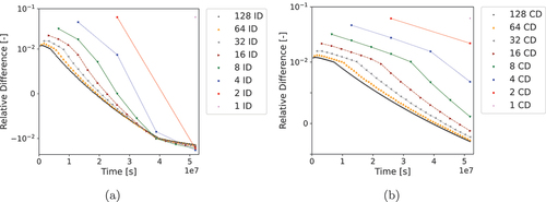
Fig. 3. Comparisons of fission density differences to the Bateman equations: (a) interval difference and (b) cumulative difference.

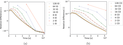
When calculating fission density or KERMA, the Bateman equations initially predict more KERMA and fissions than FE. This difference is attributed to the miscounting of decay heat by FE as the decay heat calculated at the very beginning of the first depletion interval is very close to zero when compared to the decay heat calculated at the beginning of all other depletion intervals. Consequently, the neutron flux is scaled such that fission provides almost the entirety of the rated power for the first depletion interval, when in reality as soon as fission begins, decay heat from fission products will be released. This demonstrates that the Bateman equations more accurately calculate KERMA and fission density when depleting the system using the scaled flux solution during these initial depletion intervals.

To ensure that this is true, we also evaluated the decay energy density in the system using FE and the Bateman equations, as shown in Fig. 4. Note that the ID and CD for the first depletion interval for all cases resulted in the Bateman equations calculating a value six orders of magnitude greater than FE. This is due to FE dramatically underpredicting the decay heat for the first depletion interval as mentioned previously. Overall, the decay energy density differences show that FE significantly underpredicts decay heat relative to the Bateman equations initially, with the underprediction decreasing over the course of the entire simulation. This is physically expected as the number of fissions remains relatively constant during the depletion, which results in a buildup of radioactive fission products. The short-lived fission products reach saturation and begin to provide a constant amount of decay heat while long-lived fission products steadily build up, resulting in decay heat increasing during all depletion intervals. Since FE assumes the NNDs are constant during each depletion interval, FE fails to account for this increase in decay energy while the Bateman equations succeed.

Fig. 4. Comparisons of decay energy density differences to the Bateman equations: (a) interval difference and (b) cumulative difference.

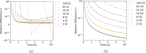
However, Fig. 4 does not explain the lower KERMA and fission density quantities calculated by the Bateman equations relative to FE in later depletion intervals. This is attributed to the decreasing macroscopic fission cross section of the fuel pin as depletion occurs and fissile nuclides are destroyed. As the macroscopic fission cross section decreases, the fission rate also decreases. Since the change in decay power released is minimal during these later depletion intervals, the decreased fission rate results in a subsequent decrease in KERMA over the course of each depletion interval. Once again, the Bateman equations account for these time-dependent effects while FE does not.

Both the Bateman equations and FE begin to converge as the number of depletion intervals increases and the length of each individual depletion interval decreases. This is to be expected based on the well-understood behavior of FE and serves as further evidence that the Bateman equations are accurately calculating the quantities of interest.

These results demonstrate that a difference of less than 7% for all tests can be observed when calculating FIMA or KERMA using FE versus the Bateman equations, with the differences decreasing to less than 2% if depletion intervals under 100 days are used. However, a quantity such as decay energy density can result in a greater than 10% difference at specific points in time for all depletion intervals tested. While other finite difference methods more accurate than FE could be used (e.g., Crank-Nicolson) and would be expected to yield better results than FE, these methods would still fail to fully account for the time dependence of the NNDs. Since the time dependence of the NNDs is explicitly modeled by the Bateman equations, calculating quantities of interest coupled to the NNDs in the Bateman equations is the more accurate method. The simplicity of calculating such values in the Bateman equations makes it relatively trivial to implement such functionality, which would then allow said quantities to benefit directly from any predictor-corrector methods implemented for the Bateman equations already.

VI. CONCLUSIONS

The process of calculating non-nuclide quantities of interest to the Bateman equations is straightforward to implement into existing depletion codes. Quantities such as damage energy, FIMA, and KERMA were calculated using the Bateman equations by modifications to Griffin. For quantities such as FIMA and KERMA, all data necessary to compute them are expected to already be present in any depletion-capable application. In the case of radiation damage, additional data, such as threshold displacement energies $E_d$ and damage-energy cross sections ${\sigma }_D$, must be made available to the code. This may present moderate challenges to existing codes that do not already have a data interface with NJOY (Ref. 12).

When tracking non-nuclide quantities of interest in the Bateman equations, the sparsity pattern of the depletion matrix may change significantly if the additional rows and columns are not added to the “correct” positions in the matrix, which can cause a degradation in the accuracy of CRAM and potentially other Bateman equation solvers depending on the linear equation solvers used for these solvers, such as SGE. Code developers must be aware of the Bateman equation solver limitations since the calculation of non-nuclide quantities was likely not anticipated when existing methods were developed. Overall, no substantial changes to an existing code are necessary.

The advantage of the proposed method is that it improves radiation damage estimates when significant radiation damage from decay and transmutation products is expected. This problem was solved only for nickel-bearing alloys using Greenwood’s correction factors. However, the production of radiation damage by transmutation products is an often overlooked issue, and Greenwood’s correction factors for radiation damage in nickel-bearing alloys are rarely used in engineering analysis. In addition, Greenwood’s correction factors work for only a single problematic nuclide, but as more materials are considered for existing and advanced reactors, the need for a method that fundamentally solves the problem without an excessive number of experiments or evaluations is growing. As interest in materials that experience very high levels of damage, such as those deployed in nuclear fusion or space applications, increases, the ability to quickly and accurately calculate radiation damage in these materials as they undergo neutron transmutation is of great value. Furthermore, there is a lack of publicly available codes capable of calculating damage-energy cross sections for polyatomic materials. More research and development work is needed here.

For other quantities of interest, the advantage is less compelling for quantities such as FIMA and KERMA as the difference between calculating the quantities using FE versus the Bateman equations typically amounted to less than 1%, except when a very small number of depletion intervals were used. When considering the uncertainties introduced by manufacturing tolerances²⁷ in real-world materials and uncertainties in nuclear data,²⁸ which can easily exceed 1%, a 1% difference in the calculated FIMA or KERMA values is within this uncertainty range. However, for quantities such as decay heat, which are much more sensitive to changes in NNDs, the differences between FE and the Bateman equations were much more significant with FE producing significantly less accurate results. Additionally, modifying the Bateman equations to compute non-nuclide number densities enables the computation of values that otherwise cannot be easily obtained via standard integration rules, such as FE. As an example, a non-nuclide representing the total number of fissions that come from only plutonium isotopes could be added, which would allow analysts and designers to easily discern what percent of their fissions is coming from specifically plutonium isotopes. Such a quantity would be challenging to accurately calculate using FE because of the time-dependent production and destruction of plutonium isotopes in uranium fuel. This is merely an example of what is possible when tracking non-nuclide quantities of interest in the Bateman equations.

Acronyms

BCMC:	=	Binary Collision Monte Carlo
CD:	=	cumulative difference
CRAM:	=	Chebyshev Rational Approximation Method
dpa:	=	displacements per atom
FE:	=	Forward Euler
FIMA:	=	fissions per initial heavy metal atom
ID:	=	interval difference
KERMA:	=	kinetic energy released per unit mass
NND:	=	nuclide number density
NRT:	=	Norgett, Robinson, and Torrens
PKA:	=	primary knock-on atom
SGE:	=	sparse Gaussian elimination

Acknowledgments

The authors thank Yaqi Wang for his support regarding implementation of this functionality in Griffin. This manuscript has been authored by Battelle Energy Alliance, LLC under contract number DE-AC07-05ID14517 with the U.S. Department of Energy. The United States Government retains and the publisher, by accepting the article for publication, acknowledges that the U.S. Government retains a nonexclusive, paid-up, irrevocable, world-wide license to publish or reproduce the published form of this manuscript, or allow others to do so, for U.S. Government purposes.

Disclosure Statement

No potential conflict of interest was reported by the authors.

Additional information

Funding

This work was supported, in part, through the Idaho National Laboratory Directed Research & Development Program and, in part, through the Nuclear Energy Advanced Modeling and Simulation program managed by the Department of Energy Office of Nuclear Energy, both of which are under DOE Idaho Operations Office Contract DE-AC07-05ID14517.

References

- H. BATEMAN, “Solution of a System of Differential Equations Occurring in the Theory of Radioactive Transformations,” Proc. Camb. Philos. Soc. Math. Phys. Sci., 15, 423 (1910).
- G. I. BELL and S. GLASSTONE, Nuclear Reactor Theory, Litton Educational Publishing, Inc. (1970).
- M. PUSA, “Rational Approximations to the Matrix Exponential in Burnup Calculations,” Nucl. Sci. Eng., 169, 2, 155 (2011); https://doi.org/10.13182/NSE10-81.
- M. GALE et al., “Using Griffin’s Transmutation Solver to Calculate Radiation Damage,” Proc. Int. Conf. Physics of Reactors 2022 (PHYSOR 2022), Pittsburgh, Pennsylvania, May 15–20, 2022, p. 836, American Nuclear Society (2022).
- G. H. KINCHIN and R. S. PEASE, “The Displacement of Atoms in Solids by Radiation,” Rep. Prog. Phys., 18, 1, 1 (1955); https://doi.org/10.1088/0034-4885/18/1/301.
- A. KONOBEYEV et al., “Evaluation of Effective Threshold Displacement Energies and Other Data Required for the Calculation of Advanced Atomic Displacement Cross-Sections,” Nucl. Energy Technol., 3, 3, 169 (2017); https://doi.org/10.1016/j.nucet.2017.08.007.
- N. JUSLIN et al., “Simulation of Threshold Displacement Energies in FeCr,” Nucl. Instrum. Methods Phys. Res., Sect. B, 255, 1, 75 (2007); https://doi.org/10.1016/j.nimb.2006.11.046.
- J. A. MASCITTI and M. MADARIAGA, “Method for the Calculation of DPA in the Reactor Pressure Vessel of Atucha II,” Sci. Technol. Nucl. Ins., 2011, 1 (2011); https://doi.org/10.1155/2011/534689.
- S. CHEN et al., “Calculation and Verification of Neutron Irradiation Damage with Differential Cross Sections,” Nucl. Instrum. Methods Phys. Res., Sect. B, 456, 120 (2019); https://doi.org/10.1016/j.nimb.2019.07.011.
- L. GREENWOOD, “A New Calculation of Thermal Neutron Damage and Helium Production in Nickel,” J. Nucl. Mater., 115, 2, 137 (1983); https://doi.org/10.1016/0022-3115(83)90302-1.
- M. NORGETT, M. ROBINSON, and I. TORRENS, “A Proposed Method of Calculating Displacement Dose Rates,” Nucl. Eng. Des., 33, 1, 50 (1975); https://doi.org/10.1016/0029-5493(75)90035-7.
- J. L. CONLIN et al., “NJOY21: Next Generation Nuclear Data Processing Capabilities,” EPJ Web Conf., 146, 09040 (2017); https://doi.org/10.1051/epjconf/201714609040.
- R. E. MACFARLANE et al., “The NJOY Nuclear Data Processing System Version 2016,” User Manual LA-UR-17-20093, Los Alamos National Laboratory (2019).
- J. LINHARD et al., “Integral Equations Governing Radiation Effects,” Matematisk-fysiske Meddelelser udgivet af Det Kongelige Danske Videnskabernes Selskab, 33, 10, (1963).
- M. ROBINSON, “Energy Dependence of Neutron Radiation Damage in Solids,” Proc. Int. Conf. Nuclear Fusion Reactors, Culham, United Kingdom, 1969, p. 364, (1969); https://www.osti.gov/biblio/4019582.
- D. SCHWEN, S. SCHUNERT, and A. JOKISAARI, “Evolution of Microstructures in Radiation Fields Using a Coupled Binary-Collision Monte Carlo Phase Field Approach,” Comput. Mater. Sci., 192, 110321 (2021); https://doi.org/10.1016/j.commatsci.2021.110321.
- W. LI et al., “Threshold Displacement Energies and Displacement Cascades in 4H-SiC: Molecular Dynamic Simulations,” AIP Adv., 9, 5, 055007 (2019); https://doi.org/10.1063/1.5093576.
- L. GREENWOOD and F. GARNER, “Hydrogen Generation Arising from the 59Ni(n, p) Reaction and Its Impact on Fission—Fusion Correlations,” J. Nucl. Mater., 233–237, 1530 (1996); https://doi.org/10.1016/S0022-3115(96)00264-4.
- A. E. ISOTALO and W. A. WIESELQUIST, “A Method for Including External Feed in Depletion Calculations with CRAM and Implementation into ORIGEN,” Ann. Nucl. Energy, 85, 68 (2015); https://doi.org/10.1016/j.anucene.2015.04.037.
- J. ORTENSI et al., “Griffin Software Development Plan,” INL/EXT-21-63185, ANL/NSE-21/23, Idaho National Laboratory and Argonne National Laboratory (2021); https://doi.org/10.2172/1845956.
- C. J. PERMANN et al., “MOOSE: Enabling Massively Parallel Multiphysics Simulation,” SoftwareX, 11, 100430 (2020); https://doi.org/10.1016/j.softx.2020.100430.
- G. MARLEAU, A. HEBERT, and R. ROY, “A User Guide for DRAGON Version 5,” User Manual IGE-355, Ecole Polytechnique de Montreal (2018).
- M. PUSA and J. LEPPÄNEN, “Solving Linear Systems with Sparse Gaussian Elimination in the Chebyshev Rational Approximation Method,” Nucl. Sci. Eng., 175, 3, 250 (2013); https://doi.org/10.13182/NSE12-52.
- K. NORDLUND et al., “Primary Radiation Damage in Materials Review of Current Understanding and Proposed New Standard Displacement Damage Model to Incorporate in Cascade Defect Production Efficiency and Mixing Effects,” Organisation for Economic Co-operation and Development, Nuclear Energy Agency (2015); http://inis.iaea.org/search/search.aspx?orig_q=RN:46066650.
- C. A. HIRST et al., “Revealing Hidden Defects Through Stored Energy Measurements of Radiation Damage,” Sci. Adv., 8, 31 (2022); https://doi.org/10.1126/sciadv.abn2733.
- O. CALVIN, S. SCHUNERT, and B. GANAPOL, “Global Error Analysis of the Chebyshev Rational Approximation Method,” Ann. Nucl. Energy, 150, 107828 (2021); https://doi.org/10.1016/j.anucene.2020.107828.
- Y. LIANG and X. WANG, “Preliminary Sensitivity and Uncertainty Analysis of Accident Tolerant Fuel in SMR,” Proc. 29th Int. Conf. Nuclear Engineering (ICONE29), Shenzhen, China, August 18–22, 2022, American Society of Mechanical Engineers (2022).
- G. ALIBERTI et al., “Nuclear Data Sensitivity, Uncertainty and Target Accuracy Assessment for Future Nuclear Systems,” Ann. Nucl. Energy, 33, 8, 700 (2006); https://doi.org/10.1016/j.anucene.2006.02.003.