Phonon Sampling Method for Inelastic Thermal Neutron Scattering Events

Abstract

Accurate representation of thermal neutron scattering in Monte Carlo transport simulations requires that the molecular vibrations of the target material be accounted for. Historically, this has been achieved by precomputing large multidimensional tables that are a function of temperature and the cosine of the scattering angle, as well as incoming and outgoing neutron energy. Most commonly used sampling techniques for thermal neutron scattering rely on large multidimensional tables, where higher resolution results in an increase in required memory and attempts to reduce memory can result in grid coarseness errors. An alternative sampling method is introduced here that is a significant departure from precomputed tables and instead relies on a more physical model of the scattering behavior. The phonon sampling method classifies neutron scattering events by the number of phonons excited/de-excited during the scattering collision. In doing so, energy exchange may be obtained via rejection sampling, and an analytical representation of the momentum exchange is obtained. This sampling method has been tested on graphite, yttrium hydride, and uranium nitride, and preliminary implementation of the phonon sampling method shows accurate results for angular and energy distributions, though resulting in up to a 40% slowdown in overall calculation time. This notable slowdown is countered, however, by a large reduction in storage (over 99% reduction compared to standard multidimensional tables).

Keywords:

• Thermal scattering
• thermal neutron
• Monte Carlo sampling

I. INTRODUCTION

The scattering behavior of thermal neutrons can greatly affect the flux profiles and criticality of many reactor systems. Thermal neutrons are characterized by their low energy (typically <5 eV), which is on the order of molecular bonds. As a result, the details of thermal neutron scattering depend on the molecular structure, unlike higher-energy neutron scattering. Thus, thermal neutron scattering data are specific to a scattering nucleus as it exists in a given media, such as “hydrogen in light water” or “carbon in crystalline graphite.” Since thermal scattering data must account for material properties as well as the target nucleus, the outgoing neutron scattering distribution can require a significant amount of prepared data, and thus may cause significant memory burdens.

Thermal neutron scattering can be elastic or inelastic, with both processes having a coherent and an incoherent component. Coherent inelastic scattering has historically not been considered due to innate difficulties in preparing such an evaluation. Thus, it is standard practice to prepare thermal neutron scattering data under the “incoherent approximation,” which assumes that coherent and incoherent inelastic scattering share the same form, effectively combining them and erasing coherent effects. This is generally a fine assumption for liquids and highly disordered polycrystalline solids,^1,2 and is used for the duration of this discussion.

In Monte Carlo neutronics simulations, thermal neutron scattering data are often prepared as large multidimensional tables, where scattering distributions are sorted for various incoming energies $E$, outgoing energies $E{ }^{\mathrm{\prime }}$, scattering cosine bins μ, and temperatures $T$. For high-precision simulations where parameter refinement may be desirable for accurate results, it is clear that the memory requirements could increase greatly. Alternatively, cumulative distribution functions (CDFs) can be constructed in both momentum exchange $\alpha$ and energy exchange $\beta$ to reduce the memory requirement burden, as was introduced by Ballinger³ and further refined by Pavlou and Ji.⁴ Additionally, a normalizing flow method for mapping the probability distributions of energy and momentum exchange has been proposed,⁵ but is not yet widely used.

The CDF method is a notable improvement to standard interpolation tables since it has reduced the required storage from four dimensions ($E$, $E{ }^{\mathrm{\prime }}$, $\mu$, and $T$) to three ($\alpha ,\beta ,T)$, while returning identical sampled distributions. However, both of these methods are held back by the fact that they are purely interpolation based in both energy and angle, such that any refinement of their respective grids could greatly increase the amount of required storage. The purpose of this paper is to introduce the phonon sampling method, which is a more flexible method of storing and sampling thermal neutron scattering data that can greatly reduce the amount of required storage while efficiently returning accurate scattering distributions. It works by sorting scattering events by the number of phonons excited or deexcited in the scattering collision, rejection sampling the energy exchange, and analytically representing the momentum exchange. The energy representation is still treated with interpolation, but the amount of memory required for highly accurate sampling distributions is reduced greatly.

This phonon sampling method was originally introduced in Ref. 6, but has since been extended and implemented in the OpenMC neutron transport Monte Carlo code for efficiency and timing statistics, and has been tested with more materials. In this paper, Sec. II covers the basics of thermal neutron scattering, including existing storage/sampling methods, Sec. III derives the basis for the phonon sampling method, and Sec. IV compares the results and efficiency of the phonon sampling method with existing methods. Note that in this work, explicit dependence on temperature is ignored such that all scattering distributions and related laws are assumed to be defined for a single temperature. Extension of the phonon sampling method to treat multiple temperatures is a necessary step, and will be discussed as future work in Sec. VII.

II. BACKGROUND

Thermal neutron scattering data are often presented in one of two forms: the double differential scattering cross section $\sigma (E\to E{ }^{\mathrm{\prime }},\mu )$, or the thermal neutron scattering law $S(\alpha ,\beta )$. The cross section is a function of incoming neutron energy $E$, outgoing neutron energy $E{ }^{\mathrm{\prime }}$, and scattering cosine $\mu$. The scattering law is a function of unitless momentum exchange $\alpha$ and unitless energy transfer $\beta$. In reality, there are two commonly used scattering laws: the symmetric form and the nonsymmetric form. For the entirety of this discussion, any mention of the scattering law $S(\alpha ,\beta )$ refers solely to the nonsymmetric form. The definitions of $\alpha$ and $\beta$ are given in Eqs. (1)(1) $\alpha =\frac{E+E{ }^{\mathrm{\prime }}-2\mu \sqrt{EE{ }^{\mathrm{\prime }}}}{A{k}_{b}T}$(1) and (2)(2) $\beta =\frac{E{ }^{\mathrm{\prime }}-E}{k_{b}T}.$(2) , where $A$ is the ratio of the scatterer mass to neutron mass, and $k_{b}T$ is the temperature in electron-volts:

(1) $\alpha =\frac{E+E{ }^{\mathrm{\prime }}-2\mu \sqrt{EE{ }^{\mathrm{\prime }}}}{A{k}_{b}T}$(1)

and

(2) $\beta =\frac{E{ }^{\mathrm{\prime }}-E}{k_{b}T}.$(2)

Since not all energy and momentum exchange combinations are physically valid, there are inherent limits for valid $\alpha ,\beta$ combinations. For a given incoming energy $E$, the minimum $\beta$ value is defined as ${\beta }_{min}=-E/k_{b}T$, and for a given $E$ and $\beta$ value, the minimum and maximum valid $\alpha$ values are defined as

(3) ${\alpha }_{min/max}(\beta ,E)=\frac{{(\sqrt{E}\mp \sqrt{E+\beta k_{b}T})}^2}{A{k}_{b}T}.$(3)

The incoherent approximation, which combines incoherent and coherent inelastic scattering such that coherent effects are effectively erased, is a standard assumption in thermal scattering evaluations. When the incoherent approximation is assumed, the intermediate scattering function (which is a Fourier transform of the scattering law) may take a Gaussian form for simple models.² The Gaussian approximation for thermal neutron scattering allows for the intermediate scattering function to be described by a Gaussian distribution for more realistic moderators, not just simple test cases. It is common practice to assume both the incoherent approximation and the Gaussian approximation when preparing thermal neutron scattering data.⁷ In doing so, the scattering law can be defined using a sum over $n$, the number of phonons excited/deexcited in a scattering collision,

(4) $S(\alpha ,\beta )={\mathrm{e}}^{-\alpha \lambda }\sum _{n=1}^{\mathrm{\infty }}\frac{{(\alpha \lambda )}^n}{n!}{T}_n(\beta ),$(4)

where $\lambda$ is the Debye-Waller coefficient and $T_n(\beta )$ is defined using the material’s phonon distribution $\rho (\beta )$,

(5) $T_n(\beta )={\int }_{-\mathrm{\infty }}^{\mathrm{\infty }}{T}_1(\beta { }^{\mathrm{\prime }})T_{n-1}(\beta -\beta { }^{\mathrm{\prime }})d\beta { }^{\mathrm{\prime }}$(5)

and

(6) $T_1(\beta )=\frac{{\mathrm{e}}^{-\beta /2}}{\lambda }\frac{\rho (\beta )}{2\beta sinh(\beta /2)}.$(6)

The Debye-Waller coefficient $\lambda$ can be defined in terms of the material’s phonon distribution $\rho (\beta )$,

(7) $\lambda ={\int }_{-\mathrm{\infty }}^{\mathrm{\infty }}\frac{\rho (\beta )}{2\beta sinh(\beta /2)}{\mathrm{e}}^{-\beta /2}d\beta .$(7)

Once the scattering law is obtained, it can be used to calculate the double-differential scattering cross section,

(8) $\sigma (E\to E{ }^{\mathrm{\prime }},\mu )=\frac{{\sigma }_b}{2k_{b}T}\sqrt{\frac{E{ }^{\mathrm{\prime }}}{E}}S(\alpha ,\beta ),$(8)

where ${\sigma }_b$ is the bound scattering cross section.

The probability distribution functions (PDFs) of the cross section can be described using the nonsymmetric scattering law,

(9) $\mathrm{P}\mathrm{D}\mathrm{F}(\beta |E)={\int }_{{\alpha }_{min}(\beta ,E)}^{{\alpha }_{max}(\beta ,E)}S(\alpha { }^{\mathrm{\prime }},\beta )d\alpha { }^{\mathrm{\prime }}$(9)

and

(10) $\mathrm{P}\mathrm{D}\mathrm{F}(\alpha |\beta ,E)=S(\alpha ,\beta ),$(10)

up to a normalizing constant. Similarly, the corresponding CDFs are defined as integrals over the PDFs,

(11) $\mathrm{C}\mathrm{D}\mathrm{F}(\beta |E)={\int }_{{\beta }_{min}(E)}^{\beta }{\int }_{{\alpha }_{min}(\beta { }^{\mathrm{\prime }},E)}^{{\alpha }_{max}(\beta { }^{\mathrm{\prime }},E)}S(\alpha { }^{\mathrm{\prime }},\beta { }^{\mathrm{\prime }})d\alpha { }^{\mathrm{\prime }}d\beta { }^{\mathrm{\prime }}$(11)

and

(12) $\mathrm{C}\mathrm{D}\mathrm{F}(\alpha |\beta ,E)={\int }_{{\alpha }_{min}(\beta ,E)}^{\alpha }S(\alpha { }^{\mathrm{\prime }},\beta )d\alpha { }^{\mathrm{\prime }},$(12)

up to a normalizing constant.

II.A. Current Methods

There are two methods of sampling thermal neutron scattering data that will be discussed here: the cross-section lookup method, which is currently implemented in the OpenMC (Ref. 8) Monte Carlo neutron transport code, and the $S(\alpha ,\beta )$ CDF method. The cross-section lookup method is referred to as such since it involves tabulation of thermal scattering data as a function of $E,E{ }^{\mathrm{\prime }},$ and $\mu$. Its implementation in OpenMC requires outgoing energy CDFs for each incoming energy, and for each $E,E{ }^{\mathrm{\prime }}$ combination, a list of equiprobable $\mu$ values. Upon selecting an incoming energy value, the $E{ }^{\mathrm{\prime }}$ CDFs may be sampled to return an $E{ }^{\mathrm{\prime }}$ value, and the equiprobable $\mu$ values are used to sample a scattering cosine for this reaction.

The $S(\alpha ,\beta )$ CDF method is a notable improvement to the cross-section lookup method, as it results in a significant reduction in required memory. By storing two dimensions, $\alpha$ and $\beta$, instead of three, $E,E{ }^{\mathrm{\prime }},\mathrm{a}\mathrm{n}\mathrm{d}\mu$, the $S(\alpha ,\beta )$ CDF method presents itself as a more lightweight option. It requires storage of the $\beta$ and $\alpha$ CDFs, defined in Eqs. (11)(11) $\mathrm{C}\mathrm{D}\mathrm{F}(\beta |E)={\int }_{{\beta }_{min}(E)}^{\beta }{\int }_{{\alpha }_{min}(\beta { }^{\mathrm{\prime }},E)}^{{\alpha }_{max}(\beta { }^{\mathrm{\prime }},E)}S(\alpha { }^{\mathrm{\prime }},\beta { }^{\mathrm{\prime }})d\alpha { }^{\mathrm{\prime }}d\beta { }^{\mathrm{\prime }}$(11) and (12(12) $\mathrm{C}\mathrm{D}\mathrm{F}(\alpha |\beta ,E)={\int }_{{\alpha }_{min}(\beta ,E)}^{\alpha }S(\alpha { }^{\mathrm{\prime }},\beta )d\alpha { }^{\mathrm{\prime }},$(12) ).

Thermal scattering data, regardless as to how they are sampled, are initially prepared by a nuclear data preprocessing code such as NJOY (Ref. 9). NJOY is a modular code that has two modules dedicated to the preparation of thermal scattering data, LEAPR and THERMR, which oversee the generation of $S(\alpha ,\beta )$ and $\sigma (E\to E{ }^{\mathrm{\prime }},\mu )$, respectfully. To calculate the scattering law, LEAPR truncates the phonon sum in Eq. (4)(4) $S(\alpha ,\beta )={\mathrm{e}}^{-\alpha \lambda }\sum _{n=1}^{\mathrm{\infty }}\frac{{(\alpha \lambda )}^n}{n!}{T}_n(\beta ),$(4) to some user-defined number of terms $N$ (typically set to 100 to 200). Some materials cannot be adequately described using so few terms, so LEAPR also makes use of the short-collision-time (SCT) approximation, which is an analytic representation of $S(\alpha ,\beta )$ that automatically turns on for selected $\alpha ,\beta$ points if deemed necessary.

When THERMR calculates $\sigma (E\to E{ }^{\mathrm{\prime }},\mu )$, it does so on a fixed $E$ grid and adaptively refines the $E{ }^{\mathrm{\prime }}$ grid according to a user-specified tolerance. Additionally, THERMR calculates a user-defined number of equiprobable $\mu$ values for each $E,E{ }^{\mathrm{\prime }}$ combination. Attention has been paid in recent years to adaptive energy grid selection for the NDEX nuclear data processing code,¹⁰ but for many applications the fixed energy grid used in THERMR is still used.

Both the cross-section lookup method and the $S(\alpha ,\beta )$ CDF method are limited by their sole reliance on grid fineness. Any refinement in their $E,E{ }^{\mathrm{\prime }},\mathrm{a}\mathrm{n}\mathrm{d}\mu$ or $\alpha ,\beta$ grids could greatly increase the corresponding memory burden. Meanwhile, coarsening of the grids could hinder accurate scattering representation. The phonon sampling method was developed in order to provide a thermal scattering sampling method that would allow for a small amount of stored data to fully represent the scattering distributions without the downfall of such grid coarseness errors.

III. PHONON SAMPLING METHOD

The summation form of the scattering law, shown in Eq. (4(4) $S(\alpha ,\beta )={\mathrm{e}}^{-\alpha \lambda }\sum _{n=1}^{\mathrm{\infty }}\frac{{(\alpha \lambda )}^n}{n!}{T}_n(\beta ),$(4) ), is particularly interesting since it is a sum over the number of phonons excited or deexcited in a scattering event. This form allows us to sort scattering events by the number of phonons interacted with and to describe their behavior in a more physically meaningful way instead of simple tabulated values. As an overview of this section, we will introduce weights that allow us to sample the number of phonons excited or deexcited in a scattering collision. Once that is obtained, the energy exchange $\beta$ can be sampled, given that $n$ phonon modes have been interacted with. Then, given a selected $n$ and $\beta$ value, we illustrate how an $\alpha$ value can be chosen via direct sampling of incomplete $\mathrm{\Gamma }$-functions.

The n’th term in the scattering law summation $S_n(\alpha ,\beta )$ is defined as

(13) $S_n(\alpha ,\beta )={\mathrm{e}}^{-\alpha \lambda }\frac{{(\alpha \lambda )}^n}{n!}{T}_n(\beta ).$(13)

Since the full scattering law is simply a sum of all $S_n(\alpha ,\beta )$ values, the weight of the n’th term can be described as

(14) $p_n(E)={\int }_{{\beta }_{min}(E)}^{{\beta }_{max}}{\int }_{{\alpha }_{min}(E,\beta { }^{\mathrm{\prime }})}^{{\alpha }_{max}(E,\beta { }^{\mathrm{\prime }})}{S}_n(\alpha { }^{\mathrm{\prime }},\beta { }^{\mathrm{\prime }})d\alpha { }^{\mathrm{\prime }}d\beta { }^{\mathrm{\prime }}.$(14)

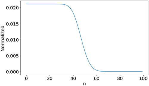
It is important to note that since the $\alpha ,\beta$ extrema are dependent on incoming energy, the $n$-weights are as well. This allows us to encompass most of the incoming-energy dependence into $p_n(E)$, which ends up being a smoothly varying function, as seen in Fig. 1, which shows $p_n(E)$ for 5 eV neutrons incident on crystalline graphite.

Fig. 1. p_n(E) for 5 eV neutrons incident on crystalline graphite. Smoothly varying sigmoid-like functions are typical for p_n(E).

III.A. Sampling β

Once a $n$ value is selected from the relative weights, a $\beta$ value can be sampled from the corresponding probability function,

(15) $\mathrm{P}\mathrm{D}\mathrm{F}(\beta |E,n)={\int }_{{\alpha }_{min}(\beta ,E)}^{{\alpha }_{max}(\beta ,E)}{S}_n(\alpha { }^{\mathrm{\prime }},\beta )d\alpha { }^{\mathrm{\prime }},$(15)

which is modeled after the $\beta$-PDF introduced in Eq. (9)(9) $\mathrm{P}\mathrm{D}\mathrm{F}(\beta |E)={\int }_{{\alpha }_{min}(\beta ,E)}^{{\alpha }_{max}(\beta ,E)}S(\alpha { }^{\mathrm{\prime }},\beta )d\alpha { }^{\mathrm{\prime }}$(9) . The definition of $S_n(\alpha ,\beta )$ can be substituted in

(16) $\mathrm{P}\mathrm{D}\mathrm{F}(\beta |E,n)=T_n(\beta ){\int }_{{\alpha }_{min}(\beta ,E)}^{{\alpha }_{max}(\beta ,E)}{\mathrm{e}}^{-\alpha { }^{\mathrm{\prime }}\lambda }\frac{{(\alpha { }^{\mathrm{\prime }}\lambda )}^n}{n!}d\alpha { }^{\mathrm{\prime }}$(16)

(17) $=T_n(\beta )w_n(\beta ,E),$(17)

and transformed such that all the $\alpha$- and $E$-dependent values are represented in $w_n(\beta ,E)$. Conveniently, $w_n(\beta ,E)$ can be represented using incomplete $\mathrm{\Gamma }$-functions

(18) $w_n(\beta ,E)=\frac{\mathrm{\Gamma }(n+1,{\alpha }_{min}(\beta ,E)\lambda )-\mathrm{\Gamma }(n+1,{\alpha }_{max}(\beta ,E)\lambda )}{\lambda n!},$(18)

meaning that once $n$ is selected, the $E$-dependent components of the $\beta$-PDF can be calculated at the time of sampling, reducing the need for $E$-dependent precomputed data.

In order to actually sample a $\beta$ value, the current implementations of the phonon sampling method use rejection sampling, with the precomputed trial functions being either Cauchy or Gaussian distributions that are dependent on both $E$ and $n$. While having $E$-dependent rejection envelopes is not preferred, since it requires a specified $E$ grid, it returns acceptable sampling efficiency and is not an overwhelming memory cost.

An added convenience facilitating this method is the generation of $T_n(\beta )$ values. Instead of precomputing and storing all $T_n(\beta )$ values for each simulation, the $T_n(\beta )$ values can be quickly generated at the beginning of each simulation via the use of Fourier transforms. Here, Eq. (5)(5) $T_n(\beta )={\int }_{-\mathrm{\infty }}^{\mathrm{\infty }}{T}_1(\beta { }^{\mathrm{\prime }})T_{n-1}(\beta -\beta { }^{\mathrm{\prime }})d\beta { }^{\mathrm{\prime }}$(5) is rewritten using the symbol $⊛$ to represent convolution,

(19) $T_n(\beta )=T_1(\beta )⊛T_{n-1}(\beta ),$(19)

and it can be proven that

(20) $F[T_n(\beta )]=F[T_1(\beta )]F[T_1(\beta ){]}^{n-1}=F[T_1(\beta ){]}^n,$(20)

where $F[]$ denotes a Fourier transform. Thus, any desired $T_n(\beta )$ value can be obtained at the beginning of a simulation by calculating

(21) $T_n(\beta )=F^{-1}[F{\left[T_1(\beta )\right]}^n],$(21)

needing only the value of $T_1(\beta )$ to be stored. When the $T_{n>1}(\beta )$ functions are obtained via Fourier transform, their grids can be coarsened to keep their memory footprint low.

Additionally, due to the iterative convolution nature of $T_n(\beta )$, for large $n$ values, $T_n(\beta )w_n(\beta )$ will tend toward Gaussian behavior. So for many materials, a $n_{cutoff}$ may be defined such that for all $n$ values above $n_{cutoff}$, the stored Gaussian distribution will not be a rejection envelope, but rather an approximation of $T_n(\beta )w_n(\beta )$, and direct sampling from said Gaussian is performed instead of rejection.

III.B. Sampling α

Once a $n$ value is sampled and a $\beta$ value is chosen via rejection sampling, an $\alpha$ value may be easily determined. The $\alpha$-PDF in the phonon sampling method is similar to that shown in Eq. (10(10) $\mathrm{P}\mathrm{D}\mathrm{F}(\alpha |\beta ,E)=S(\alpha ,\beta ),$(10) ), but with $n$ being specified,

(22) $\mathrm{P}\mathrm{D}\mathrm{F}(\alpha |\beta ,n,E)=S_n(\alpha ,\beta ),$(22)

which, when rewritten to include the full definition of $S_n(\alpha ,\beta )$, appears as

(23) $\mathrm{P}\mathrm{D}\mathrm{F}(\alpha |\beta ,E,n)={\mathrm{e}}^{-\alpha \lambda }\frac{{(\alpha \lambda )}^n}{n!}{T}_n(\beta ),$(23)

and the corresponding CDF is defined as

(24) $\mathrm{C}\mathrm{D}\mathrm{F}(\alpha |\beta ,E,n)={\int }_{{\alpha }_{min}(\beta ,E)}^{\alpha (\beta ,E)}{\mathrm{e}}^{-\alpha { }^{\mathrm{\prime }}\lambda }\frac{{(\alpha { }^{\mathrm{\prime }}\lambda )}^n}{n!}{T}_n(\beta )d\alpha { }^{\mathrm{\prime }}.$(24)

Since $\beta$ and $n$ have already been selected by this point, the $T_n(\beta )$ value may be safely removed, leaving an equation that can again be represented via the use of incomplete $\mathrm{\Gamma }$-functions,

(25) $\mathrm{C}\mathrm{D}\mathrm{F}(\alpha |\beta ,n,E)=\frac{1}{\lambda }[\mathrm{\Gamma }(n+1,{\alpha }_{min}(\beta ,E)\lambda )-\mathrm{\Gamma }(n+1,\alpha \lambda )],$(25)

which allows for $\alpha$ to be obtained via direct sampling.

III.C. Method Overview

In this section, a summary and overview of the phonon sampling method is provided. In its current implementation, the phonon sampling method accepts a small number of inputs, which are outlined in Table I.

TABLE I Precomputed Values for the Phonon Sampling Method

Precomputed Value	Description
$T_1(\beta )$	Introduced in Eq. (6(6) $T_1(\beta )=\frac{{\mathrm{e}}^{-\beta /2}}{\lambda }\frac{\rho (\beta )}{2\beta sinh(\beta /2)}.$(6) )
$p_n(E)$	Introduced in Eq. (14(14) $p_n(E)={\int }_{{\beta }_{min}(E)}^{{\beta }_{max}}{\int }_{{\alpha }_{min}(E,\beta { }^{\mathrm{\prime }})}^{{\alpha }_{max}(E,\beta { }^{\mathrm{\prime }})}{S}_n(\alpha { }^{\mathrm{\prime }},\beta { }^{\mathrm{\prime }})d\alpha { }^{\mathrm{\prime }}d\beta { }^{\mathrm{\prime }}.$(14) )
Rejection envelopes	For sampling $T_n(\beta )w_n(\beta )$,dependent on $n$ and $E$
$n_{cutoff}$ (optional)	For $n>n_{cutoff}$, $T_n(\beta )w_n(\beta )$ is assumed to be Gaussian.
$n$ grid used (optional)	Coarse $n$ grid, useful for some materials
$\lambda$	Debye-Waller coefficient

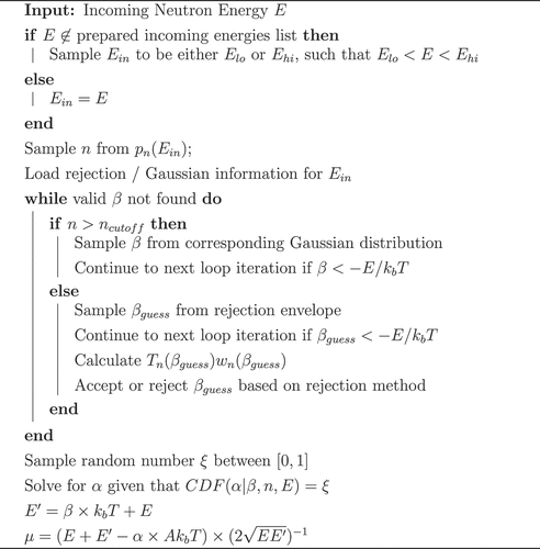
Once these values are obtained and stored, they may be used to sample thermal scattering distributions in a Monte Carlo simulation as outlined in Algorithm 1. Algorithm 1: Phonon Sampling Method Overview

Note that $p_n(E)$ and the rejection envelope parameters are the only values that are dependent on incoming energy. Since $p_n(E)$ is a smoothly varying function, it could be condensed and/or approximated as a continuous function. Additionally, the only other memory intensive input is $T_1(\beta )$, which for the materials considered in this paper [uranium nitride (UN), crystalline graphite, and yttrium hydride (YH₂)] requires only 100 to 500 points.

As previously mentioned, the phonon sampling method relies heavily on classifying scattering events according to the number of phonons excited or deexcited. Elastic scattering, which corresponds to the creation or destruction of zero phonons, is generally treated separately from inelastic scattering. Coherent elastic scattering relies on crystallographic data and could not be sufficiently described by the phonon sampling method. Incoherent elastic scattering could be considered a special case of the phonon sampling method, but implementation of such a case is not explored in the present work.

IV. RESULTS AND COMPARISON

To best illustrate the effectiveness of the phonon sampling method, we compare it to both the standard interpolation table method and to the $S(\alpha ,\beta )$ PDFs. The phonon sampling method was implemented into the OpenMC neutron transport simulation code,⁸ and can be compared against the standard cross-section lookup that is commonly used in Monte Carlo codes, including OpenMC. For the following comparisons, OpenMC was modified to return the single-scattering distributions resulting from these two methods, which are plotted alongside the PDFs obtained using the scattering law.

This comparison uses three materials at room temperature: nitrogen in UN, carbon in crystalline graphite, and hydrogen in YH₂. Typically, the phonon sampling method uses an incoming energy grid of approximately 20 values spaced between ${10}^{-5}$ and 5.0 eV. Scattering data obtained using the THERMR module of NJOY are typically prepared for 118 incoming energy points, ranging between ${10}^{-5}$ and 10.0 eV (Ref. 7). For the purposes of this comparison, the input data for the phonon sampling method were prepared on this same energy grid.

IV.A. Carbon in Crystalline Graphite

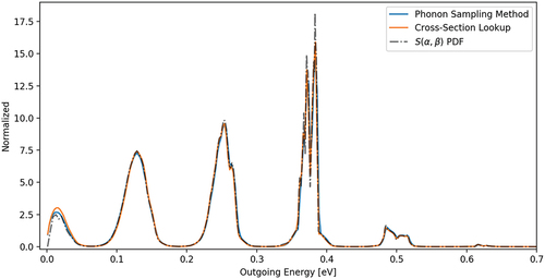
Crystalline graphite is a relatively simple material for the phonon sampling method to describe. Figure 1 shows that at 5.0 eV, graphite requires that only 60 to 70 phonon sum terms be used, meaning that the scattering behavior of crystalline graphite can be accurately represented by the phonon sampling method while using a relatively small amount of prepared memory. To illustrate the strong agreement between the phonon sampling method and standard methods, Fig. 2 shows the outgoing single-scatter energy distributions for 1.2 eV neutrons incident on crystalline graphite, as calculated using the three methods of interest: phonon sampling, cross section lookup, and $S(\alpha ,\beta )$ PDF. Figure 2 shows the phonon sampling method and the cross-section lookup method returning nearly identical single-scatter outgoing energy distributions. Note that there are small discontinuities in the $S(\alpha ,\beta )$ PDF near 0.73 and 0.82 eV, which are due to coarseness in the $\alpha$ grids used.

Fig. 2. Single-scatter energy distributions for 1.2 eV neutrons incident on crystalline graphite.

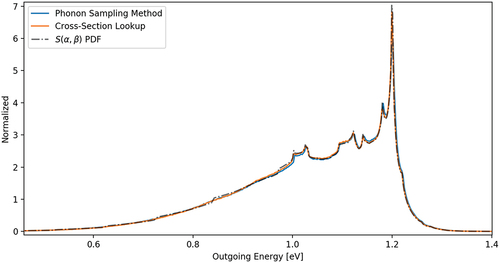
Note that an incoming neutron energy of 1.2 eV is relatively high for the thermal energy range. It is used as a validation point for the purposes of this paper because it allows for a sufficient amount of phonon structure to be clearly seen in the outgoing energy distribution.

One of the notable advantages of the phonon sampling method is that it allows for direct sampling of the angular distribution, given that $n$ and $\beta$ have already been selected. To highlight this benefit, the single-scattering angular distribution for 1 eV neutrons scattering off of graphite to energies between 0.905 and 0.910 eV is shown in Fig. 3. The phonon sampling method tallies are compared with the standard cross-section lookup tallies and plotted alongside the corresponding $\alpha$-PDF that was transformed to represent $\mu$.

Fig. 3. Single-scatter cosine distributions for 1.0 eV neutrons that scatter on crystalline graphite to energies between 0.905 and 0.910 eV. The α-PDF is transformed to represent μ values.

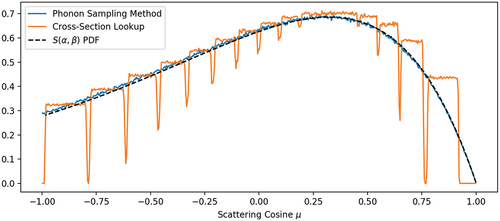
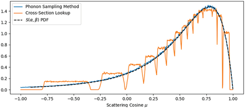
While the results of the phonon sampling method and the $S(\alpha ,\beta )$-PDF agree well, they both behave quite differently than the distribution obtained using the standard cross-section lookup method. The reason for this discrepancy is that the method currently used by OpenMC, and perhaps by other Monte Carlo sampling codes, is to sample an equiprobable cosine ${\mu }_i$, and then select a $\mu$ for a scattering event from a bin of width

(26) $\frac{1}{2}min[{\mu }_i-{\mu }_{i-1},{\mu }_{i+1}-{\mu }_i]$(26)

centered about ${\mu }_i$. Thus, single-scattering angular distributions can have steps and dips where the equiprobable bins do not have sufficient overlap. While the effects of this behavior are likely overshadowed by other factors in a larger-scale calculation, they are inaccuracies nonetheless and have the potential to cause misrepresentation in some structures.

IV.B. Hydrogen in YH₂

The phonon distribution for H in YH₂ is particularly interesting since it consists of one main peak near 0.125 eV. Because of this singular peak, the outgoing energy distributions from a single collision appear as equally spaced peaks, such that a peak at $E_{in}\pm a\times 0.125\mathrm{e}\mathrm{V}$ indicates the destruction/creation of $a$ phonons. This behavior is clearly seen in Fig. 4, which shows the outgoing energy distributions for 0.5 eV neutrons incident on H in YH₂. Note that 0.5 eV is in the prepared incoming energy list, meaning that interpolation across incoming energy is not required. All three cases considered show strong agreement.

Fig. 4. Single-scatter energy distributions for 0.5 eV neutrons incident on H in YH₂.

Additionally, it is worthwhile to consider the effects of energy interpolation on the scattering distribution. To show this, we have the outgoing energy distribution for 1.2 eV neutrons incident on H in YH₂, shown in Fig. 5, since 1.2 eV is not in the prepared list of incoming energies used for this paper. The cross-section lookup used by default in OpenMC does not perform interpolation for incoming energies, but rather uses the data of the nearest energy. This creates a noticeable shift in the locations of the peaks, and while this error is often overshadowed by other effects, it is worthwhile to take note of.

Fig. 5. Single-scatter energy distributions for 1.2 eV neutrons incident on H in YH₂. Since 1.2 eV is not in the prepared incoming energy list, interpolation was required.

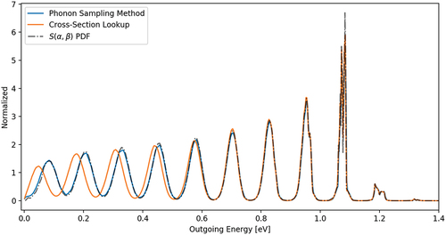
Note that, similar to the crystalline graphite outgoing energy comparison shown in Fig. 2, the Y in YH₂ distributions in Fig. 5 are compared for an incoming energy that is relatively high in the thermal spectrum. This energy was chosen to highlight the phonon structure resultant from multiple phonon excitations of the optical hydrogen peak, which manifests in the outgoing energy distribution as peaks spaced approximately 0.124 eV apart.

IV.C. Nitrogen in UN

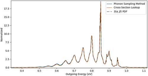
With the rise of interest in advanced nuclear fuels, attention has been paid to UN. The thermal scattering capabilities of N in UN have been considered, and are used as a validation case for the phonon sampling method. The outgoing energy distributions for 0.9 eV neutron single-scatter events are shown in Fig. 6. Note that the outgoing energy peaks, which indicate individual phonon events, agree in both shape and position between the three methods.

Fig. 6. Single-scatter energy distributions for 0.9 eV neutrons incident on N in UN.

The outgoing angular distributions can also be compared, as was done for the YH₂ comparison. For a beam of 0.9 eV neutrons that scattered to outgoing energies between 0.8518 and 0.8526 eV, the angular distributions were tallied. The resulting distribution is shown in Fig. 7. Note that the distribution obtained via the cross-section lookup method again exhibits plateaued behavior with significant dips due to the equiprobable $\mu$ sampling method. This behavior is avoided by the phonon sampling method due to the direct sampling of $\alpha$.

Fig. 7. Single-scatter cosine distributions for 0.9 eV neutrons incident on N in UN are considered. The scattering cosines for neutrons with outgoing energies between 0.8518 and 0.8526 eV are shown. The α-PDF corresponding to an outgoing energy of 0.8522 eV is plotted for comparison.

Close examination of the scattering distributions for the three chosen materials—carbon in crystalline graphite, hydrogen in YH₂, and nitrogen in UN—all indicate that the phonon sampling method is able to accurately return outgoing energy and angular distributions for thermal scattering events while avoiding currently accepted errors, such as interpolation errors and nonphysical behavior exhibited in sampled angular distributions.

V. MEMORY

To illustrate the benefits of the phonon sampling method, a memory usage comparison is provided between it and the cross-section lookup method that is currently implemented in OpenMC. Comparisons against the $S(\alpha ,\beta )$-CDF method are not provided since its memory requirements can vary greatly depending on the coarseness of the $\alpha ,\beta$ grids.

Phonon sampling input files were generated for the three materials of interest: graphite, H in YH₂, and N in UN. Coarsened $n$ grids and $p_n(E)$ grids were used when applicable to decrease the amount of required space. The number of required floating point values for each material is shown in Table II. Unless otherwise indicated, the columns indicate the total number of floating point values needed across all incoming and outgoing energies and that the incoming energies range from ${10}^{-5}$ to 4.9 eV. The approximate memory size is also provided, where double-precision floating point values are assumed for $p_n(E)$ and single precision is assumed for all other values.

TABLE II Number of Floating Point Values Required by the Phonon Sampling Method in Order to Describe the Thermal Scattering Behavior of Select Room Temperature Materials

	$E_{in}$	$T_1(\beta )$	$p_n(E)$	Rejection Sampling Parameters	Other	Total	Approximate Memory (kB)
Graphite	109	401	1431	4293	5	6239	29.9
H in YH2	109	265	1090	3597	5	5066	24.0
N in UN	109	229	1438	4314	5	6095	29.4

From the information in Table II, we find that graphite requires approximately 57 values per incoming energy, while H in YH₂ requires approximately 46 values and N in UN requires approximately 56. These memory requirements can be compared against typical storage requirements for the cross-section lookup method. The ENDF/B-VIII.0 HDF5 library generated for OpenMC available in Ref. 11 was used for the memory comparison. These HDF5 libraries, which store data for incoming energies, outgoing energies, and for each $E,E{ }^{\mathrm{\prime }}$ pairing, store a number of equiprobable $\mu$ values. A summary of these values is shown in Table III. Note that for every incoming energy, both an outgoing energy grid and a corresponding CDF are stored, meaning that since crystalline graphite stores a total of 88 336 outgoing energies, the total number of floating point values for energy selection is 176 672. For each incoming and outgoing energy pair, a set number of equiprobable scattering cosines is stored (typically 16).

TABLE III Number of Floating Point Values Stored in the HDF5 OpenMC Libraries to Describe the Thermal Scattering Behavior of Various Room-Temperature Materials

	$E_{in}$	Outgoing Energies	$\mu$	Total	Approximate Memory (kB)
Graphite	109	176 672	1 413 376	1 590 157	12 423
H in YH2	109	325 090	2 600 720	2 925 919	22 858
N in UN	109	284 918	2 279 344	2 564 371	20 034

VI. EFFICIENCY

VI.A. Pin Cell Geometries

Phonon sampling is a relatively new method being proposed, and in its current implementation is not expected to match the speed of standard sampling techniques, as it utilizes a rejection sampling routine and intermediate calculations. However, to illustrate its current performance, average run times for pin cell geometry calculations are compared.

Three pin cell geometries were considered, each testing the thermal scattering treatment for the materials of interest (graphite, YH₂, and UN). Each geometry consisted of infinite concentric cylinders placed in square lattices. The outer radii for the fuel, gap, and cladding were 0.39, 0.40, and 0.46 cm, respectively, and the moderator filled the remaining area. The uranium in the fuel was 3% ²³⁵U and 97% ²³⁸U, and the pin pitch was 2.0 cm. In order to test the graphite and YH₂ cases, UO₂ was set as the fuel, and thermal scattering effects were only considered for the moderator (C in crystalline graphite or H in YH₂). For the UN case, the moderator was set to be YH₂, and thermal scattering effects were only considered for N in UN. These three cases were modeled with OpenMC using 200 batches, 40 inactive batches, and 100 000 particles per batch. The resulting values for $k_{eff}$ and their standard deviations are given in Table IV.

TABLE IV $k_{eff}$ Values for the Pin Cell Calculations*

	C in Graphite	H in YH2	N in UN
Phonon sampling	$0.90113\pm 0.00022$	$0.88678\pm 0.00019$	$0.90300\pm 0.00021$
Standard treatment	$0.90139\pm 0.00022$	$0.88681\pm 0.00020$	$0.90327\pm 0.00018$
Absolute difference	$0.00026\pm 0.00031$	$0.00003\pm 0.00028$	$0.00027\pm 0.00028$

*±indicates one standard deviation.

In order to compare the timing statistics, the same three pin cell geometries were considered, and were run using the phonon sampling method and the standard OpenMC treatment. For each geometry, 10 runs using each method were performed in alternating sequence to ensure a fair comparison. For these calculations, 100 batches were used, with 20 inactive batches and 20 000 particles per batch. The total run times were summed over all 10 iterations and are shown in Table V.

TABLE V OpenMC Models of the Three Pin Cell Geometries Using Either the Phonon Sampling Method or the Standard Treatment*

	C in Graphite	H in YH2	N in UN
Phonon sampling	2949 s	1333 s	1028 s
Standard treatment	2595 s	959 s	1009 s
Relative slowdown	13.6%	38.9%	1.9%

*Ten runs of each were performed, and the total run time across these ten runs is summed and provided in seconds.

As can be seen by the timing efficiency comparisons provided in Table VI, use of the phonon sampling method can result in slowdowns ranging from approximately 2% to nearly 40%, depending on the moderating material being described. This variation in timing efficiency is largely due to the rejection sampling scheme used to select the energy exchange parameter $\beta$. Since the rejection envelopes used to initially select ${\beta }_{guess}$ values may vary in how well they match the actual behavior of $T_n(\beta )w_n(\beta )$, some materials may experience larger rejection rates than others.

TABLE VI $k_{eff}$ Values for the ICSBEP Criticality Benchmarks*

	heu-met-inter-006 Case 1	heu-sol-therm-001 Case 1
Phonon Sampling	$0.99450\pm 0.00009$	$0.98465\pm 0.00010$
Standard Treatment	$0.99461\pm 0.00009$	$0.98481\pm 0.00010$
Absolute difference	$0.00011\pm 0.00013$	$0.00016\pm 0.00014$

*±indicates one standard deviation.

VI.B. International Criticality Safety Benchmark Evaluation Project Geometries

Further accuracy and efficiency tests can be performed using critical reactor benchmarks, such as those outlined in the International Criticality Safety Benchmark Evaluation Project¹² (ICSBEP). Two ISCBEP benchmarks were selected: heu-met-inter-006 (case 1) and heu-sol-therm-001 (case 1), which were used to test the graphite and the uranium-nitrogen scattering behavior, respectively. heu-met-inter-006 is from the ZEUS Criticality Experiments, and heu-sol-therm-001 (case 1) is comprised of minimally reflected cylinders of uranyl nitrate.

Note that both of these ICSBEP benchmark models come with their limitations. For instance, the heu-met-inter-006 model lacks a strong thermal flux, which limits its applicability in illustrating the accuracy of the phonon sampling method. It is, however, an effective tool in demonstrating the sampling efficiency for a nonthermal reactor model in which thermal scattering models are still considered. Similarly, the heu-sol-therm-001 model contains uranyl nitrate as opposed to UN, meaning that applying the N in UN thermal scattering treatment is not an accurate physical representation. This benchmark is selected nonetheless so as to allow for the results of the OpenMC method to be compared against the phonon sampling method. Since it is recognized that the heu-sol-therm-001 model is being modeled with a thermal scattering treatment that is not physically representative, comparison against experimentally measured values is not provided.

Both cases were run in OpenMC for a total of 1100 batches (100 inactive), with 100 000 particles per batch. For each benchmark case, the phonon sampling method and the standard OpenMC method were used, and the resultant $k_{eff}$ values are displayed in Table VI. Note that since the phonon sampling method and the standard sampling method follow different trains of logic in their implementation, they were unable to match exactly for a given seed, and were instead prone to statistical uncertainty. With this possibility for statistical variation prevalent, the agreement in $k_{eff}$ values shown in Table VI is particularly strong, with the absolute difference between values being well within two standard deviations for both benchmark cases considered. Again, it is worth highlighting that minimal disagreement was expected for the heu-met-inter-006 model since its thermal flux is relatively weak.

The timing efficiency of the phonon sampling method can be further explored by comparing the total time required by each method for the two benchmark tests. The total amount of time required by the simulations is shown in Table VII.

TABLE VII Total Calculation Time for OpenMC Modeling of ICSBEP Geometries

	heu-met-inter-006 Case 1	heu-sol-therm-001 Case 1
Phonon sampling	4684.1 s	2731.6 s
Standard treatment	4662.7 s	2752.7 s

When comparing the timing results from the ICSBEP models (Table VII) with those from the pin cell runs (Table V), it becomes evident that use of the phonon sampling method can affect the simulation run time quite differently, depending on the material geometry and moderator composition. In a more complex simulated system where a variety of effects contribute to the run time, the effect of thermal scattering sampling on the run time can be more easily washed out, potentially reducing its effect significantly. This is especially true for the considered ICSBEP cases, where either the neutron flux is not highly thermal (heu-met-inter-006) or there are competing moderating nuclides that are not considered in the aforementioned comparison (heu-sol-therm-001).

VI.C. Transient Reactor Test Facility Model

In addition to the pin cell and ICSBEP geometries, a model from the Transient Reactor Test Facility (TREAT) was also used to study the effectiveness of the phonon sampling method. The TREAT reactor has been studied in a variety of configurations, one of which is referred to as the minimum critical mass configuration (MCM). Details of this configuration are available in Ref. 13. The TREAT reactor is surrounded by two types of graphite reflectors: a permanent graphite reflector surrounding the core and graphite plugs above and below the active fuel region. The fuel itself is uranium embedded in a graphite matrix. With this reflector and fuel composition, the TREAT reactor is heavily graphite moderated and has a strong thermal spectrum, thereby serving as a useful tool for illustrating the viability of the phonon sampling method for use in thermal reactor systems. The MCM core is simulated in an eigenvalue calculation for 150 batches (50 inactive) with 50 000 particles per batch. The resultant eigenvalues are shown in Table VIII. As can be seen in the results table, the absolute difference between the two $k_{eff}$ values is less than two standard deviations from each other, illustrating statistical similarity. Note that some differences between the accumulated results are to be expected due to effects, such as interpolation of incoming neutron energy, grid coarseness errors, and statistical variation, that may all contribute to minor disagreements.^a The timing comparison for the MCM TREAT reactor model is provided in Table IX.

TABLE VIII $k_{eff}$ Values of the MCM TREAT Reactor Model*

	MCM TREAT Model
Phonon sampling	$1.01080\pm 0.00038$
Standard treatment	$1.00971\pm 0.00044$
Absolute difference	$0.00109\pm 0.00058$

*±indicates one standard deviation.

TABLE IX Total Calculation Time for OpenMC Modeling of TREAT MCM Reactor Model

	MCM TREAT Model
Phonon sampling	67 198 s
Standard treatment	64 648 s

Note that use of the phonon sampling method increases the required run time by approximately 4%, which is significantly less than the 13.6% slowdown reported in Table V. This decrease in extra required run time is likely due to the fact that a full-core reactor calculation requires a significant number of additional calculations, which tends to wash out the additional costs associated with the phonon sampling method.

VII. CONCLUSION

In this discussion, the phonon sampling method was introduced as a lightweight alternative to standard sampling practices. The two most common sampling methods that are typically utilized have been denoted as the cross-section lookup method and the CDF method. The cross-section lookup method is a widely used sampling technique that prepares large scattering tables as a function of $E,E{ }^{\mathrm{\prime }},\mathrm{a}\mathrm{n}\mathrm{d}\mu$. Due to the large multidimensional tables required by this method, the $S(\alpha ,\beta )$-CDF sampling method was developed, where CDFs of $\alpha$ and $\beta$ (parameters representing unitless momentum and energy exchange, respectively) could be used to obtain scattering distributions. Since the CDF method effectively eliminated a dimension in the tables, it is notable for its significant reduction in required storage. However, both methods can suffer from grid coarseness errors in their stored data, where an increase in accuracy via grid refinement comes at the cost of increased memory usage. The phonon sampling method aims to circumvent this restriction by representing thermal scattering in a more physically meaningful way, by categorizing scattering events by the number of phonon modes excited/deexcited. Doing so allows for partial analytical representations of the momentum exchange, which can greatly alleviate grid coarseness errors.

The phonon sampling method has been shown to represent the scattering behavior for carbon in crystalline graphite, hydrogen in YH₂, and nitrogen in UN adequately. In its current implementation, the phonon sampling method can be considerably slower due to its internal rejection sampling routine. In order to better compete with more commonly used methods, the phonon sampling method will require more extensive testing in criticality calculations as well as validation with additional materials. Future improvements to the phonon sampling method may include an expansion to multiple temperatures, removal/acceleration of the rejection sampling requirement, and potentially an incorporation of the SCT approximation, which can be used to alleviate the burden of representing events that produce/destroy many phonons. In total, the phonon sampling method shows great promise in its ability to return accurate thermal neutron scattering distributions, while allowing for a relatively small amount of prepared data to be provided.

Acknowledgments

The authors would also like to thank Carl Haugen and Travis Labossiere Hickman for their work in developing the model of the MCM TREAT core.

Disclosure Statement

No potential conflict of interest was reported by the authors.

Additional information

Funding

This work was performed with support from the U.S. Department of Energy Naval Reactors Program Rickover Fellowship. Any opinions, findings, or conclusions expressed in this paper are those of the authors and do not necessarily reflect the views of the Naval Reactors Program.

Notes

^a The differences in incoming energy treatment, while not specifically emphasized in this work, can contribute to noticeable effects in the simulated behavior of a reactor system. The single-scatter outgoing energy distribution depicted in Fig. 5 illustrates how (for intermediate energy points for which data have not been explicitly prepared), the calculated scattered behavior can differ between the methods.

References

- G. PLACZEK and L. VAN HOVE, “Interference Effects in the Total Neutron Scattering Cross-Section of Crystals,” Il Nuovo Cimento (1955–1965), 1, 1, 233 (1955); https://doi.org/10.1007/BF02731767.
- M. M. R. WILLIAMS, The Slowing Down and Thermalization of Neutrons, North-Holland Publishing Company (1966).
- C. BALLINGER, “The Direct S (α, β) Method for Thermal Neutron Scattering.” Proc. Int. Conf. on Mathematics and Computation, Reactor Physics, and Environmental Analysis, Portland, OR, April 30 - May 4 (1995).
- A. T. PAVLOU and W. JI, “On-the-Fly Sampling of Temperature-Dependent Thermal Neutron Scattering Data for Monte Carlo Simulations,” Ann. Nucl. Energy, 71, 411 (2014); https://doi.org/10.1016/j.anucene.2014.04.028.
- B. FORGET and A. ALHAJRI, “Normalizing Flows for Thermal Scattering Sampling,” Ann. Nucl. Energy, 170, 108974 (2022); https://doi.org/10.1016/j.anucene.2022.108974.
- A. TRAINER and B. FORGET, “Development of a Phonon-Based Sampling Method for Thermal Neutron Scattering Data.” Proc. PHYSOR, Pittsburgh, PA, May 15-2 (2022).
- R. MACFARLANE et al., “The NJOY Nuclear Data Processing System, Version 2016,” LA-UR-17-20093, Los Alamos National Laboratory (2016).
- P. K. ROMANO et al., “OpenMC: A State-of-the-Art Monte Carlo Code for Research and Development,” Ann. Nucl. Energy, 82, 90 (2015); https://doi.org/10.1016/j.anucene.2014.07.048.
- R. MACFARLANE et al., “The NJOY Nuclear Data Processing System, Version 2016.” Technical Report, Los Alamos National Laboratory (2017).
- J. WORMALD, J. THOMPSON, and T. TRUMBULL, “Implementation of an Adaptive Energy Grid Routine in NDEX for the Processing of Thermal Neutron Scattering Cross Sections,” Ann. Nucl. Energy, 149, 107773 (2020); https://doi.org/10.1016/j.anucene.2020.107773.
- OPENMC DEVELOPMENT TEAM, “OpenMC Official Data Libraries,” (2015); https://openmc.org/official-data-libraries/.
- J. D. BESS et al., “The 2019 Edition of the ICSBEP Handbook,” Technical Report, Idaho National Laboratory (2019).
- J. D. BESS and M. D. DEHART, “Baseline Assessment of TREAT for Modeling and Analysis Needs,” Technical Report, Idaho National Laboratory (2015).