Physics-Informed Neural Network with Fourier Features for Radiation Transport in Heterogeneous Media

Abstract

Typical machine learning (ML) methods are difficult to apply to radiation transport due to the large computational cost associated with simulating problems to create training data. Physics-informed Neural Networks (PiNNs) are a ML method that train a neural network with the residual of a governing equation as the loss function. This allows PiNNs to be trained in a low-data regime in the absence of (experimental or synthetic) data. PiNNs also are trained on points sampled within the phase-space volume of the problem, which means they are not required to be evaluated on a mesh, providing a distinct advantage in solving the linear Boltzmann transport equation, which is difficult to discretize. We have applied PiNNs to solve the streaming and interaction terms of the linear Boltzmann transport equation to create an accurate ML model that is wrapped inside a traditional source iteration process. We present an application of Fourier Features to PiNNs that yields good performance on heterogeneous problems. We also introduce a sampling method based on heuristics that improves the performance of PiNN simulations. The results are presented in a suite of one-dimensional radiation transport problems where PiNNs show very good agreement when compared to fine-mesh answers from traditional discretization techniques.

Keywords:

• Physics-informed neural network
• radiation transport
• Fourier Features

I. INTRODUCTION

Often, machine learning (ML) processes are data driven and rely on the acquisition of a large amount of data in order to be trained. ML has been applied to many fields in science and engineering,^1,2 where these training data, be they empirical measurements or synthetic results generated from simulations, can be costly to obtain in terms of resources (human time and hardware/software costs). In addition, data-driven ML processes may not yet be fully generalizable or explainable, and purely data-driven methods may not extrapolate well due to observational biases.³ Therefore, there is a need for incorporating governing laws [e.g., partial differential equations (PDEs)] into the learning process in order to increase the robustness of ML techniques in low-data regimes and to improve their explainability. When concerned with the transport of radiation (neutrons, photons, etc.) through a background medium, one has to discretize a fairly high-dimensional phase-space in order to track particles with respect to their position, energy, and direction of motion.

In three-dimensional geometries, this results in a six-dimensional phase-space, making the discretization of the associated linear Boltzmann transport equation a challenging task, even on modern computer architectures.⁴ This potentially exacerbates the low-data regime issues mentioned above, as numerical solutions to the transport equation are costly to obtain.

In this work, we present the application of physics-informed neural networks (PiNNs) to the radiation transport equation. PiNNs can be categorized as a deep-learning technique based on (deep) feedforward neural networks. Typically, the input layer of a PiNN consists of one neuron per independent phase-space variable, followed by several hidden layers with a significant number of neurons per layer (which makes this a deep-learning approach), and finally an output layer consisting of one neuron (for scalar PDEs) or several neutrons (for vector PDEs). At the heart of a PiNN feedforward neural network is the mechanism by which the parameters (weights and biases) of the network are obtained. This is directly related to the definition of the neural network’s loss function. The loss function incorporates (1) the governing laws themselves (i.e., the PDE’s residual in the phase-space volume), thus making this a physics-informed approach; (2) boundary conditions; (3) initial conditions (for time-dependent problems); and (4) measurements (if any).

PiNNs were first proposed in Ref. 5 and utilize the automatic differentiation capabilities of the neural network to evaluate differential operators occurring in the PDE, hence enabling the construction of the loss function (i.e., residual) associated with the PDE. It must be noted that the differentiation is, therefore, taken with respect to the input layer variables (e.g., position and time, as needed) to build the residual of the PDE at selected phase-space points. The standard backpropagation algorithm is employed for this task. In order to optimize the network’s parameters, automatic differentiation is also employed with respect to the network’s parameters (this is the more commonly understood use of backpropagation in neural networks).

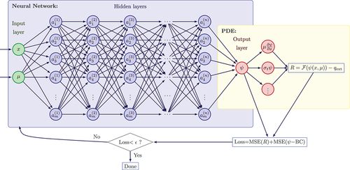
Parameter optimization (i.e., the training of the PiNN) relies on standard optimization algorithms in ML, specifically, Adam optimization⁶ and limited-memory BFGS (L-BFGS), a quasi-Newton gradient-based optimization algorithm.⁷ A typical PiNN architecture as well as elements of the process behind PiNNs are shown in Fig. 1. In this schematic, the neural network consists of two input neurons [a two-dimensional (2-D) phase-space described by independent variables $x$ and $\mu$]; this is followed by $n$ hidden layers, each with $m$ neurons, and an output layer for the scalar variable $\psi (x,\mu )$ that is the solution of the PDE $\mathcal{F}(\psi (x,\mu ))=q$. The residual of the PDE at sampled points in the phase-space volume is built, as well as the boundary residual. Both residuals are then used in the definition of a loss function whose minimization process trains the parameters of the neural network.

Fig. 1. PiNN example: The neural network consists of two input neurons (in the case of a 2-D phase-space), followed by $n$ hidden layers, each with $m$ neurons, and an output layer for the scalar variable, solution of the PDE $\mathcal{F}(\psi (x,\mu ))=q$. The residual of the PDE at sampled points in the phase-space volume is built, as well as the boundary residual. Both residuals are then in the definition of a loss function whose minimization process trains the parameters of the neural network.

Automatic differentiation is used at two instants: first, to evaluate the residual of the PDE (as governing laws often contain spatial derivatives of the solution variables) and second, to optimize the weights and biases of the network. Given that the PDE residual is evaluated at sampled points in the phase-space volume, a PiNN solution does not require meshing of the geometry, and hence, PiNN techniques to solve PDEs are often thought of as a family of meshless methods.

PiNNs have already been applied to a wide variety of disciplines in science and engineering; see, for instance, the recent review paper³ and the references therein. Despite early successes in using PiNNs to solve governing laws using ML, several limitations currently exist. For example, a solid mathematical explanation of PiNNs is still lacking, which precludes understanding why PiNNs can oftentimes fail. In addition, the large computational cost of training a neural network means that PiNNs currently are much slower than traditional PDE solvers. However, once trained, PiNNs evaluate solutions at any point within the phase-space much faster than traditional solvers.

In Ref. 8, it is noted that PiNNs can struggle to converge when the solution exhibits high frequencies or multiscale features (or simply highly heterogeneous material properties, per our own observations); the authors showed that fully connected PiNNs converge to Gaussian processes in the infinite width limit for linear PDEs. The convergence rate of the total training error of a PiNN model was analyzed in terms of the spectrum of its neural tangent kernel.

In Ref. 9, the authors employ Fourier Feature networks that use a simple Fourier Feature mapping to increase the ability of fully connected neural networks (fcNNs) to learn high-frequency functions (this approach was originally proposed in Ref. 10). For advection-dominated problems, additional techniques have been proposed to improve the accuracy of PiNNs. In Ref. 11 the authors argue that the parameter optimization that takes place in the PiNN learning process does not respect the space-time causality of physical systems where information propagates at a finite speed; to respect the physical causality during the learning process, they proposed to reformulate the definition of the loss function so that learning (and thus parameter optimization) accounts for physical causality.

In another study, the authors of Ref. 12 also note the failure of PiNNs to converge for “complicated” PDEs. They were able to overcome some of the challenges by developing adaptive sampling strategies used in training the PiNNs. They hypothesized that training of PINNs relies on a successful “propagation” of solution from initial and/or boundary condition points to interior points, and they subsequently proposed evolutionary sampling algorithms to incrementally add sampling points in the location of high residuals.

In Ref. 13, the governing laws are rewritten in a Lagrangian framework, so that the PiNNs now include two distinct branches: one that learns the low-dimensional characteristics curve and one that solves for the state variables along the characteristics. This approach, coined Lagrangian PiNNs, was shown to outperform the traditional PiNNs in the Eulerian framework for a wide class of convection-diffusion problems.

Finally, another approach developed to combat the lack of high-accuracy solutions of PiNNs consists of adding a discriminator network in addition to the PiNN. In this adversarial approach, called competitive PiNNs, the discriminator is trained (rewarded) for predicting mistakes the PiNN commits.

The remainder of this paper is as follows. In Sec. II, we review the radiation transport equation and provide some details related to the standard scattering source iteration (SI) solution process that is also employed within our PiNN definitions. In Sec. III, we provide details on the PiNNs (phase-space inputs, definition of loss function, and handling of scattering terms). We pay particular attention to improvements made to handle heterogeneous material via a combination of pass-through and Fourier Feature neurons after the input layer. Results are provided in Sec. IV for various one-dimensional (1-D) radiation transport benchmarks. Conclusions and outlook are proposed in Sec. V.

II. RADIATION TRANSPORT GOVERNING LAWS

The linear Boltzmann equation for neutral particles, in steady state, with isotropic scattering and external sources and single-speed formalism, is given by

(1a) $\begin{array}{rl}& \vec{\mathrm{\Omega }}\cdot \vec{\mathrm{\nabla }}\mathrm{\Psi }(\vec{r},\vec{\mathrm{\Omega }})+{\sigma }_t(\vec{r})\mathrm{\Psi }(\vec{r},\vec{\mathrm{\Omega }})=\frac{{\sigma }_s(\vec{r})}{4\pi }\mathrm{\Phi }(\vec{r})+\frac{Q(\vec{r})}{4\pi }\\ & \mathrm{\forall }\vec{r}\in \mathcal{D}\mathrm{a}\mathrm{n}\mathrm{d}\vec{\mathrm{\Omega }}\in {\mathcal{S}}^2,\end{array}$(1a)

supplemented with boundary conditions

(1b) $\begin{array}{rl}& \mathrm{\Psi }(\vec{r},\vec{\mathrm{\Omega }})={\mathrm{\Psi }}^{inc}(\vec{r},\vec{\mathrm{\Omega }})\\ & \mathrm{\forall }\vec{r}\in \mathrm{\partial }{\mathcal{D}}^{-}=\{\vec{r}\in \mathrm{\partial }\mathcal{D}\mathrm{s}\mathrm{u}\mathrm{c}\mathrm{h}\mathrm{t}\mathrm{h}\mathrm{a}\mathrm{t}\vec{\mathrm{\Omega }}\cdot \vec{n}(\vec{r})<0\},\end{array}$(1b)

where

$\mathrm{\Psi }(\vec{r},\vec{\mathrm{\Omega }})$	=	= angular flux solution of the transport equation
$\vec{r}$	=	=  spatial position
$\vec{\mathrm{\Omega }}$	=	=  direction of motion
${\sigma }_t,$ ${\sigma }_s$	=	= total and scattering macroscopic cross sections, respectively
$Q$	=	=  external volumetric source
${\mathrm{\Psi }}^{inc}$	=	=  incoming surface source
$\mathcal{D}$	=	=  spatial domain
${\mathcal{S}}^2$	=	=  unit sphere.

The scalar flux $\mathrm{\Phi }$ is the angular integral of the angular flux:

(2) $\mathrm{\Phi }(\vec{r})={\int }_{4\pi }d\mathrm{\Omega }\mathrm{\Psi }(\vec{r},\vec{\mathrm{\Omega }}).$(2)

In 1-D slab geometry, the streaming operator $\vec{\mathrm{\Omega }}\cdot \vec{\mathrm{\nabla }}$ devolves to $\mu \frac{\mathrm{\partial }}{\mathrm{\partial }x}$, with $\mu =\vec{\mathrm{\Omega }}\cdot {\vec{e}}_x$.

For classical discretization techniques, Eq. (1)(1a) $\begin{array}{rl}& \vec{\mathrm{\Omega }}\cdot \vec{\mathrm{\nabla }}\mathrm{\Psi }(\vec{r},\vec{\mathrm{\Omega }})+{\sigma }_t(\vec{r})\mathrm{\Psi }(\vec{r},\vec{\mathrm{\Omega }})=\frac{{\sigma }_s(\vec{r})}{4\pi }\mathrm{\Phi }(\vec{r})+\frac{Q(\vec{r})}{4\pi }\\ & \mathrm{\forall }\vec{r}\in \mathcal{D}\mathrm{a}\mathrm{n}\mathrm{d}\vec{\mathrm{\Omega }}\in {\mathcal{S}}^2,\end{array}$(1a) is discretized in space and angle. We recall briefly these discretization approaches here, although a PiNN solution process is meshless and does not require the notion of grid or meshes. For traditional techniques, an angular quadrature is often used to discretize the angular variable and to carry out angular integrations:

(3a) $\begin{array}{rl}& \left({\vec{\mathrm{\Omega }}}_d\cdot \vec{\mathrm{\nabla }}+{\sigma }_t(\vec{r})\right){\mathrm{\Psi }}_d(\vec{r})=\frac{{\sigma }_s(\vec{r})}{4\pi }\mathrm{\Phi }(\vec{r})+\frac{Q(\vec{r})}{4\pi }\\ & \mathrm{\forall }\vec{r}\in \mathcal{D}\mathrm{a}\mathrm{n}\mathrm{d}{\vec{\mathrm{\Omega }}}_d\in {\mathcal{S}}^2,\end{array}$(3a)

supplemented with boundary conditions:

$\begin{array}{rl}& {\mathrm{\Psi }}_d(\vec{r})={\mathrm{\Psi }}_{\mathrm{d}}^{\mathrm{i}\mathrm{n}\mathrm{c}}(\vec{r})\\ & \mathrm{\forall }\vec{r}\in \mathrm{\partial }{\mathcal{D}}^{-}=\{\vec{r}\in \mathrm{\partial }\mathcal{D}\mathrm{s}\mathrm{u}\mathrm{c}\mathrm{h}\mathrm{t}\mathrm{h}\mathrm{a}\mathrm{t}{\vec{\mathrm{\Omega }}}_d\cdot \vec{n}(\vec{r})<0\},(3\mathrm{b})\end{array}$

with the scalar flux being evaluated as

(3c) $\mathrm{\Phi }(\vec{r})=\sum _{d=1}^{N_{\mathrm{\Omega }}}{w}_d{\mathrm{\Psi }}_d(\vec{r}).$(3c)

The angular quadrature is given by the direction-weight pairs $({\vec{\mathrm{\Omega }}}_d,w_d)$ with $(1\le d\le N_{\mathrm{\Omega }}$), and the approach is referred to in the literature as a discrete ordinates angular discretization.¹⁴ Note that ${\mathrm{\Psi }}_d(\vec{r})\equiv \mathrm{\Psi }(\vec{r},{\vec{\mathrm{\Omega }}}_d)$. For spatial discretization, it is standard to use finite differencing (such as the diamond scheme, Ref. 15) or discontinuous finite elements.^16,17 We refer the reader to these references for additional spatial discretization details. In what follows, we will keep using the spatially undiscretized expressions of Eq. (3)(3a) $\begin{array}{rl}& \left({\vec{\mathrm{\Omega }}}_d\cdot \vec{\mathrm{\nabla }}+{\sigma }_t(\vec{r})\right){\mathrm{\Psi }}_d(\vec{r})=\frac{{\sigma }_s(\vec{r})}{4\pi }\mathrm{\Phi }(\vec{r})+\frac{Q(\vec{r})}{4\pi }\\ & \mathrm{\forall }\vec{r}\in \mathcal{D}\mathrm{a}\mathrm{n}\mathrm{d}{\vec{\mathrm{\Omega }}}_d\in {\mathcal{S}}^2,\end{array}$(3a) for brevity.

With regard to solution techniques, both the traditionally discretized transport equation and its PiNN equivalent will employ a standard Source Iteration (SI) approach. In SI, the scattering source is lagged at the previous iteration $\mathrm{\ell },$ and the solution process is as follows:

(1) Given old values for the scalar flux, obtain new angular fluxes:

(4a) $\begin{array}{rl}& \left({\vec{\mathrm{\Omega }}}_d\cdot \vec{\mathrm{\nabla }}+{\sigma }_t(\vec{r})\right){\mathrm{\Psi }}_d^{(\mathrm{\ell }+1)}(\vec{r})=\frac{{\sigma }_s(\vec{r})}{4\pi }{\mathrm{\Phi }}^{(\mathrm{\ell })}(\vec{r})+\frac{Q(\vec{r})}{4\pi }\\ & \mathrm{\forall }\vec{r}\in \mathcal{D}\mathrm{a}\mathrm{n}\mathrm{d}{\vec{\mathrm{\Omega }}}_d\in {\mathcal{S}}^2,\end{array}$(4a)

for $1\le d\le N_{\mathrm{\Omega }}$.

(2) Update the scalar flux:

(4b) ${\mathrm{\Phi }}^{(\mathrm{\ell }+1)}(\vec{r})=\sum _{d=1}^{N_{\mathrm{\Omega }}}{w}_d{\mathrm{\Psi }}_d^{(\mathrm{\ell }+1)}(\vec{r}).$(4b)

III. PiNNs: DEFINITIONS AND ADVANCED FEATURES

In this section, we detail the specifics of our application of PiNNs to radiation transport. In Sec. III.A, we describe our implementation of PiNN for each angular direction and how the angular flux estimates for each PiNN are used to update the scalar flux through SIs. In Sec. III.B, we give a brief overview of fully connected neural network architecture. In Sec. III.C, we detail our specific application of Fourier Features to improve PiNN performance in heterogeneous problems. In Sec. III.D, we give a description of the training of neural networks as well as how PiNNs differ from traditional supervised neural networks. In Sec. III.E, we explain how PiNNs leverage automatic differentiation to calculate the partial derivatives in the governing equation (here, the radiation transport equation). Finally, in Sec. III.F, we explain our sampling methods that lead to better training performance in heterogeneous problems. These specific methods allow for PiNNs to be applied to the more difficult heterogeneous problems that a vanilla implementation of PiNNs struggles to solve effectively, if at all.

III.A. Source Iteration and PiNNs

As is described in Sec. II, SI is often employed to solve radiation transport problems. In order to easily solve for the scalar flux, a PiNN for each direction in the angular quadrature is devised. Specifically, the PiNN is substituted for the inversion of the left-hand side operator of Eq. (4a)(4a) $\begin{array}{rl}& \left({\vec{\mathrm{\Omega }}}_d\cdot \vec{\mathrm{\nabla }}+{\sigma }_t(\vec{r})\right){\mathrm{\Psi }}_d^{(\mathrm{\ell }+1)}(\vec{r})=\frac{{\sigma }_s(\vec{r})}{4\pi }{\mathrm{\Phi }}^{(\mathrm{\ell })}(\vec{r})+\frac{Q(\vec{r})}{4\pi }\\ & \mathrm{\forall }\vec{r}\in \mathcal{D}\mathrm{a}\mathrm{n}\mathrm{d}{\vec{\mathrm{\Omega }}}_d\in {\mathcal{S}}^2,\end{array}$(4a) ; this is shown in Eq. (5)$\begin{array}{rl}& \mathrm{P}\mathrm{i}\mathrm{N}{\mathrm{N}}_d:\mathrm{C}\mathrm{o}\mathrm{m}\mathrm{p}\mathrm{u}\mathrm{t}\mathrm{e}{\mathrm{\Psi }}_d^{(\mathrm{\ell }+1)}\mathrm{g}\mathrm{i}\mathrm{v}\mathrm{e}\mathrm{n}\left\{\frac{{\sigma }_s(\vec{r})}{4\pi }{\mathrm{\Phi }}^{(\mathrm{\ell })}(\vec{r})+\frac{Q(\vec{r})}{4\pi }\right\}\\ & \mathrm{f}\mathrm{o}\mathrm{r}d\in [1,N_{\mathrm{\Omega }}],(5)\end{array}$:

$\begin{array}{rl}& \mathrm{P}\mathrm{i}\mathrm{N}{\mathrm{N}}_d:\mathrm{C}\mathrm{o}\mathrm{m}\mathrm{p}\mathrm{u}\mathrm{t}\mathrm{e}{\mathrm{\Psi }}_d^{(\mathrm{\ell }+1)}\mathrm{g}\mathrm{i}\mathrm{v}\mathrm{e}\mathrm{n}\left\{\frac{{\sigma }_s(\vec{r})}{4\pi }{\mathrm{\Phi }}^{(\mathrm{\ell })}(\vec{r})+\frac{Q(\vec{r})}{4\pi }\right\}\\ & \mathrm{f}\mathrm{o}\mathrm{r}d\in [1,N_{\mathrm{\Omega }}],(5)\end{array}$

where the left-hand side of the equation represents the output of the PiNN trained while being driven by the current total (i.e., extraneous + scattering) source evaluated using the lagged scalar flux ${\mathrm{\Phi }}^{(\mathrm{\ell })}$. Once all angular fluxes ${\mathrm{\Psi }}_d^{(\mathrm{\ell }+1)}$ have been obtained by training $N_{\mathrm{\Omega }}$ different PiNNs, we can update the scalar flux by using Eq. (4b)(4b) ${\mathrm{\Phi }}^{(\mathrm{\ell }+1)}(\vec{r})=\sum _{d=1}^{N_{\mathrm{\Omega }}}{w}_d{\mathrm{\Psi }}_d^{(\mathrm{\ell }+1)}(\vec{r}).$(4b) as before. The scalar flux is then used to update the right-hand side of the governing equation, as traditionally done in SIs. Hence, in our scheme, the SIs are wrapped around the classical transport sweeps; however, PiNNs are used and trained in order to obtain those angular fluxes (one PiNN per angular direction). Note that between each update of the angular flux, the PiNN is not initialized again but instead uses the final state of the previous SI. Because of this, both the SI error and training error are reduced together instead of needing to fully retrain each PiNN at each SI. This also means that the number of epochs required to fully train each PiNN decreases with each SI, as will be illustrated in our numerical results.

III.B. Neural Network Architecture

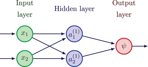
As shown in Fig. 1, fcNNs are composed of an input layer, hidden layers, and an output layer. A fcNN can have any number of inputs and outputs, and in general, both can be normalized or scaled. There will be one neuron for each input and output, and each hidden layer can contain any number of neurons. Between hidden layers $l-1$ and $l$, there will be a set of weights $W^{(l)}\in {\mathbb{R}}^{(m_{l-1}\times m_l)}$, where $m_l$ is the number of neurons in layer $l$. The weights are used to generate a linear combination of the previous layer’s output. This linear combination will form the input for the next layer. In addition, each neuron in layer $l$ also has a bias, i.e., $b^{(l)}\in {\mathbb{R}}^{m_l}$. Nonlinear activation functions $a$ (typically, sigmoid, tanh, and ReLU) transform the input of each neuron. Hence, the output of a given layer in a network from the output of the previous layer is given in Eq. (6)(6) $z^{(l)}=a(W^{(l)}{z}^{(l-1)}+b^{(l)}),$(6) :

(6) $z^{(l)}=a(W^{(l)}{z}^{(l-1)}+b^{(l)}),$(6)

with $z^{(l)}\in {\mathbb{R}}^{m_l}$. Given a total of $n$ hidden layers, the fully connected network of Fig. 1 can be mathematically described as

$f:{\mathbb{R}}^{di{m}_i}\to {\mathbb{R}}^{di{m}_o}$

$f(x)=g_o\circ z^{(n)}\circ z^{(n-1)}\dots \circ z^{(1)}\circ g_i,$

with $di{m}_i$ and $di{m}_o$ the dimension of the input and output layers (in Fig. 1, these are 2 and 1), and the input/output layer functions $g_i=W^{(i)}x+b^{(i)}$ and $g_o=W^{(o)}{z}^{(n)}+b^{(o)}$. Once trained (i.e., all weights and biases are optimized), the computation of this expression can be done very quickly, even for large networks. The main issue in utilizing a fcNN comes in the determination of the weights and biases, which form the set of trainable variables, hereinafter denoted as $\theta$. This determination is achieved through training, which is explained in Sec. III.D.

III.C. Fourier Features

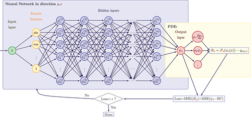
The benefit of Fourier Features to improve PiNNs’ representation of high-frequency functions or problems with multiscale features is presented in Ref. 9. Drastically heterogeneous problems are generally difficult for PiNNs to represent, and Fourier Features promise to alleviate this issue. The general architecture for a neural network with Fourier Features is shown in Fig. 2, where Fourier Features project the neural network input by applying sines and cosines of various frequencies as shown in Eq. (7)(7) $f(x)=[sin({\omega }_{i}x)cos({\omega }_{i}x)],$(7) :

(7) $f(x)=[sin({\omega }_{i}x)cos({\omega }_{i}x)],$(7)

Fig. 2. Radiation transport PiNN in direction ${\mu }_d$ with Fourier Features added.

where ${\omega }_i$ is the $i$’th randomly sampled frequency sampled from the Gaussian distribution $\mathcal{N}(0,{\sigma }^2),$ where $\sigma$ is a hyperparameter of the network. In some implementations of Fourier Features, ${\omega }_i$ are trained alongside the weights and biases of the network; however, in this paper they will be kept fixed at the sampled values.

A further modification to the Fourier Feature algorithm proposed is the addition of bypass neurons to the Fourier Feature layer of the network. These neurons will simply pass the input directly as is, instead of projecting in sine or cosine functions. The addition of bypass neurons leads to $2\times N_{FF}+N_{BN}$ total neurons in the Fourier Feature layer, where $N_{FF}$ is the number of Fourier Feature pairs and $N_{BN}$ is the number of bypass neurons.

III.D. Neural Network Training

Neural networks are trained by optimizers that adjust the weights and biases in order to find an optimal version of the network. This optimal version is determined by the minimization of a loss function. In supervised fcNNs, the loss function is classically an error metric compared to a known or desired solution. However, for PiNNs, the loss function instead is based on the residual of the PDE under consideration. The method by which PiNNs are able to evaluate this residual is given later, in Sec. III.E. For now, it suffices to consider that the PiNN loss function is given by the sum of an interior residual and a boundary residual, as shown in Eq. (8)(8) $\mathcal{L}(\theta )=R_{int}+R_{BC},$(8) :

(8) $\mathcal{L}(\theta )=R_{int}+R_{BC},$(8)

where $R_{int}$ and $R_{BC}$ are the internal and boundary residuals, evaluated at the sampled internal points and the boundaries, respectively, and $\theta$ is the set of trainable parameters, as described in Sec. III.B. This choice of loss function is what differentiates PiNNs from traditional fcNNs. Each contribution to the loss function is evaluated at points sampled from the domain. The sampling of the domain is further described in Sec. III.F. Once this loss function is evaluated, the weights and biases of the neural network must be updated by the optimizer function. The two main optimizers used for neural networks are the first-order Adam optimizer and the second-order LBFGS optimizer. The goal of optimizers can be described as finding $\theta { }^{\mathrm{\prime }}$ such that

(9) $\theta { }^{\mathrm{\prime }}=\underset{\theta \in \mathrm{\Theta }}{argmin}\mathcal{L}(\theta ),$(9)

with $\mathrm{\Theta }$ being the set of all possible values of the trainable parameters. Both optimizers attempt to find $\theta { }^{\mathrm{\prime }}$ by using descent directions ${\mathrm{\partial }}_{\theta }\mathcal{L}$ in order to calculate the update to the trainable parameters. The evaluation of the sensitivity of the loss to each parameter (${\mathrm{\partial }}_{\theta }\mathcal{L}$) is achieved via backpropagation.

III.E. PDE Residual Calculation

PiNNs require a method for calculating the residual of the PDEs under consideration. To do so, PiNNs leverage automatic differentiation to calculate the partial derivatives found in the expression of the PDE. Automatic differentiation is also used in the training of traditional data-driven feedforward networks. This section will give a brief view of automatic differentiation; see Ref. 18 for additional details. The specific type of automatic differentiation used is reverse accumulation, which is composed of two steps: forward pass and backpropagation. The forward pass is simply an evaluation of the neural network where values for each neuron are saved to be used in the second step. When evaluating the forward pass for PiNNs, the values of the input must be saved as well. Once all of the relevant values are saved, it is then possible to perform a backpropagation stage.

Backpropagation allows the derivative of the output to be calculated with respect to any value within the network by leveraging the chain rule. While it is common to see backpropagation used with respect to parameters, we describe below how the derivative of the network’s output (the angular flux in direction $d$ in our case) with respect to input variables is computed. For example, to calculate $\frac{\mathrm{\partial }\psi }{\mathrm{\partial }{x}_1}$ from Fig. 3, the first application of the chain rule is shown in Eq. (10)(10) $\frac{\mathrm{\partial }\psi }{\mathrm{\partial }{x}_1}=\sum _{i=1}^2\frac{\mathrm{\partial }\psi }{\mathrm{\partial }{a}_i^{(1)}}\frac{\mathrm{\partial }{a}_i^{(1)}}{\mathrm{\partial }{x}_1}.$(10) :

(10) $\frac{\mathrm{\partial }\psi }{\mathrm{\partial }{x}_1}=\sum _{i=1}^2\frac{\mathrm{\partial }\psi }{\mathrm{\partial }{a}_i^{(1)}}\frac{\mathrm{\partial }{a}_i^{(1)}}{\mathrm{\partial }{x}_1}.$(10)

Fig. 3. Small example of a neural network.

This equation can be further expanded using the chain rule again, yielding

(11) $\frac{\mathrm{\partial }\psi }{\mathrm{\partial }{x}_1}=\sum _{i=1}^2\frac{\mathrm{\partial }\psi }{\mathrm{\partial }{a}_i^{(1)}}\frac{\mathrm{\partial }{a}_i^{(1)}}{\mathrm{\partial }{z}_i}\frac{\mathrm{\partial }{z}_i}{\mathrm{\partial }{x}_1},$(11)

where $z_i$ is the value of neuron $i$ before the activation function is applied. It is then possible to analytically calculate $\frac{\mathrm{\partial }{a}_i^{(1)}}{\mathrm{\partial }{z}_i}$ for a given activation function $a_i$. It can then be very easily found that the other two terms simply are the weights $W^{(l)}$ for their respective layer $l$. This yields the final formula for $\frac{\mathrm{\partial }\psi }{\mathrm{\partial }{x}_1}$, shown in Eq. (12)(12) $\frac{\mathrm{\partial }\psi }{\mathrm{\partial }{x}_1}=\sum _{i=1}^2{W}_i^{(0)}\sigma { }^{\mathrm{\prime }}(z_i)W_i^{(1)}.$(12) , where the total contribution of each individual contribution is summed:

(12) $\frac{\mathrm{\partial }\psi }{\mathrm{\partial }{x}_1}=\sum _{i=1}^2{W}_i^{(0)}\sigma { }^{\mathrm{\prime }}(z_i)W_i^{(1)}.$(12)

Here, this approach is used in PiNNs in order to calculate the term containing $\frac{\mathrm{\partial }\mathrm{\Psi }}{\mathrm{\partial }x}$ in the formula for $R_{int}$. Then, it is simple to sum the contribution from each term appearing in the PDE, yielding a complete method to compute the residual of said PDE:

(13) $R_{int,d}=\sum _{i=0}^{N_{int}}{\left({\mu }_d\frac{\mathrm{\partial }{\mathrm{\Psi }}_{d,i}}{\mathrm{\partial }x}+{\sigma }_t{\mathrm{\Psi }}_{d,i}-\frac{{\sigma }_s}{4\pi }{\mathrm{\Phi }}_i-\frac{Q_i}{4\pi }\right)}^2,$(13)

where ${\mathrm{\Psi }}_{d,i}$ and ${\mathrm{\Phi }}_i$ are the angular flux in direction $d$ and the scalar flux, both evaluated at internal point $x_i$ ${\mathrm{\Psi }}_{d,i}$ is the output of the PiNN for direction $d$. Next, for the complete evaluation of the loss $\mathcal{L}(\theta )$, the boundary residual $R_{BC}$ is computed as follows:

(14) $R_{BC,d}=\sum _{j=0}^{N_{BC}}({\mathrm{\Psi }}_{BC,d,j}-{\mathrm{\Psi }}_{d,j}{)}^2,$(14)

where ${\mathrm{\Psi }}_{BC,d,j}$ and ${\mathrm{\Psi }}_{d,j}$ are the boundary condition and the angular flux (in direction $d$) evaluated at the boundary point $x_j$. Again, ${\mathrm{\Psi }}_{d,j}$ is the output of the PiNN for direction $d$. The sampling of the internal and boundary points is described in the next section.

III.F. Point Sampling

Point sampling is necessary to evaluate the loss function, and the sampling points are divided into boundary points and internal points. In this section, the different sampling approaches used in this paper are discussed. Boundary points are simply divided evenly between the two boundaries (left/right) of the 1-D problems considered in this paper. They will not be discussed further. The simplest sampling approach for internal points is a random uniform sampling of a given number of points $N_i$ inside each material zone $i$ in the problem domain. This method has advantages in its simplicity, but it usually does not perform as well at material interfaces, especially for highly heterogeneous configurations. As a first attempt to improve the performance of PiNNs, sampling is done such that there is a sufficient density of training points, given the mean-free-path thickness of each material zone $i$.

Equation (15)(15) $N_{i,mfp}=max\left(\alpha \frac{h_i{\mathrm{\Sigma }}_{t,i}}{{\mu }_{min}},N_i\right),$(15) shows the formula for $N_{i,mfp}$, the number of points in material zone $i$ that ensures a density in each mean free path of material:

(15) $N_{i,mfp}=max\left(\alpha \frac{h_i{\mathrm{\Sigma }}_{t,i}}{{\mu }_{min}},N_i\right),$(15)

where ${\mu }_{min}$ is the smallest positive cosine of the angular directions, $h_i$ is the width of zone $i$, and $\alpha$ is a parameter that determines how many points will be sampled per mean free path. This sampling method ensures that each part of the domain is sampled enough to resolve any material boundaries or other heterogeneities. However, in problems where there is a large difference in material properties, there can still be difficulties in converging the solution well for all regions. We propose a heuristic, whereby the number of samples per region obtained from mean-free-path considerations is modified as follows. The number of points sampled is further increased in certain regions according to their influence, denoted ${\gamma }_i$, on the loss function. The influence ${\gamma }_i$ is calculated with Eq. (16)(16) ${\gamma }_i=max\left(\frac{1}{{\mathrm{\Sigma }}_{t,i}},ϵ\right)+max\left(\frac{{\mu }_{min}}{h_i},ϵ\right),$(16) :

(16) ${\gamma }_i=max\left(\frac{1}{{\mathrm{\Sigma }}_{t,i}},ϵ\right)+max\left(\frac{{\mu }_{min}}{h_i},ϵ\right),$(16)

where $ϵ$ is a parameter that ensures that the number of points sampled will not become too large in spatially thin, optically thin, or void zones of the problem. The number of points to be sampled in each zone can be calculated using the zonal influences, as is shown in Eq. (17)(17) $N_{i,is}=\frac{{\gamma }_{max}}{{\gamma }_i}\times N_{i,mfp},$(17) :

(17) $N_{i,is}=\frac{{\gamma }_{max}}{{\gamma }_i}\times N_{i,mfp},$(17)

with ${\gamma }_{max}={max}_i({\gamma }_i)$. Heuristically, this zonal influence-based sampling ensures that the loss for an error in any zone would be roughly equivalent. This property ensures that the error in each zone will be minimized at the same rate leading the problem to converge similarly in all zones.

IV. RESULTS

In this section, we present numerical results for our PiNN implementation applied to a set of five radiation benchmark problems taken from Ref. 19. The traditional Reed problem²⁰ is Problem 5 in our suite of test cases. All problems are evaluated with an $S_8$ quadrature except for Problem 3 and Problem 4’, which are only evaluated with an $S_2$ quadrature (we used a lower-order angular quadrature in order to illustrate the effects of Fourier Features on the angular flux in Problem 3; the same conclusions hold, of course, for an $S_8$ angular quadrature as well). All problems use vacuum boundary conditions.

All of the PiNNs used to solve these problems employ the same architecture. They all start with a Fourier Feature projection layer followed by five fully connected layers. Each of the fully connected layers contains 64 neurons, and the Fourier Feature layers have 10 bypass neurons, 64 sine projection neurons, and 64 cosine projection neurons, for a total of 138 neurons in the Fourier layer. Each of the fully connected layers uses the swish activation function, and the inputs are normalized between zero and one before the Fourier Feature projection layer. Each PiNN was also trained using a combination of the Adam and LBFGS optimizers.

For each problem, the extent of each material spatial zone and the material properties of that zone (absorption and isotropic scattering macroscopic cross sections) will be given in a table. The flux solutions of the PiNNs are compared against a fine-mesh finite difference (FD) solution (here, we employed diamond-differencing with a fine enough mesh).

In terms of computing time, the FD traditional solvers yield the answer in a mere few seconds at most; training a PiNN on a single CPU on a modern desktop computer takes on the order of 60 min; with GPU acceleration, the training time is on the order of 20 min. These sample timing results were produced using the free version of the Google Colaboratory run-time environment for consistency in our comparisons. We note that the large factor in compute times between neural network methods and traditional solvers is consistent with observations reported elsewhere; see, for instance, Ref. 21.

IV.A. Problem 1

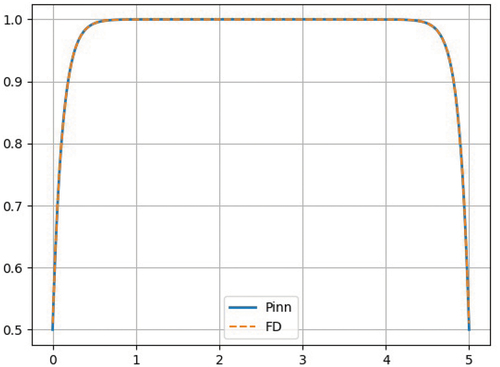
Problem 1 is a homogeneous slab containing a pure absorber. The extent of each spatial zone and the material properties are given in Table I. The results of the PiNNs compared to the results of a FD solution are shown in Fig. 4, where we observe excellent agreement between the two solutions. Homogeneous problems like this one are fairly easy to converge (even without using Fourier Features). The remainder of the test cases includes problems with more variations in the solution where the benefit of Fourier Features will become obvious.

TABLE I Problem 1 Definition

$x$	${\mathrm{\Sigma }}_a$	${\mathrm{\Sigma }}_s$	$q$
[0,5]	5	0	5

Fig. 4. Scalar flux for Problem 1: PiNN and FD solutions.

IV.B. Problem 2

This test case includes the presence of scattering and is still a homogeneous material; however, the source is present in only one of the two material zones. The extent of each spatial zone and the material properties are given in Table II. The presence of scattering requires SIs to solve the problem. The results of the PiNNs compared to the results of a FD solution are shown in Fig. 5. There is good agreement between these two solutions. This problem proves that our approach of wrapping the SI around the PiNN solution is appropriate.

TABLE II Problem 2 Definition

$x$	${\mathrm{\Sigma }}_a$	${\mathrm{\Sigma }}_s$	$q$
[0,0.5]	2.5	2.5	5
[0.5,1]	2.5	2.5	0

Fig. 5. Scalar flux for Problem 2: PiNN and FD solutions.

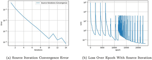
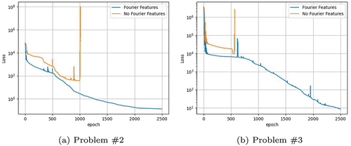
In Fig. 6a, we show the SI convergence (measured as the successive differences in scalar flux estimates). In Fig. 6b, we show a plot of the loss value versus epochs while training one of the neural networks (for one of the directions in the $S_N$ quadrature); in this graph, the sharp increase in the loss corresponds to a new scattering source provided from the SI process; between these SI updates, the loss decreases rapidly. Because the loss-versus-epochs graph (Fig. 6b) shows the loss for only one of the PiNNs, the loss error displayed does not directly correlate to the scalar flux error of Fig. 6a. As SIs continue, the number of epochs required for this error to decrease to its previous value (before the scattering source update) decreases until the scattering source converges.

Fig. 6. Training error with scattering.

IV.C. Problem 3

This problem and Problem 4 are both heterogeneous problems that will be employed to demonstrate the strengths and weaknesses of our neural network implementation. The extent of each spatial zone and the material properties are given in Table III.

TABLE III Problem 3 Definition

$x$	${\mathrm{\Sigma }}_a$	${\mathrm{\Sigma }}_s$	$q$
[0,1]	50	0	5
[1,5]	1	0	0

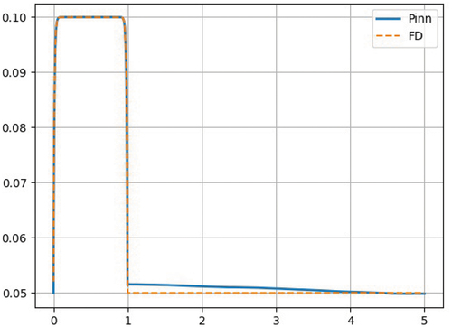
Because of how heterogeneous this problem is, it is a good test case to illustrate the strength of the Fourier Features approach used in our neural network. The scalar flux solution for the PiNN with Fourier Features is shown in Fig. 7a. This can be compared to the scalar flux solution obtained without Fourier Features, shown in Fig. 8a. This discrepancy in the solution can be explained by Fig. 8b, where the PiNN solution is more diffusive than the FD solution. PiNNs without Fourier Features fail to represent the more heterogeneous problems because the networks return diffusive answers. This shows the strong advantage of PiNNs including Fourier Features especially when the problem is strongly heterogeneous.

Fig. 7. Problem 3 with Fourier Features: PiNN and FD solutions.

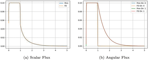
Fig. 8. Problem 3 without Fourier Features: PiNN and FD solutions.

Another undesirable behavior present in the PiNNs without Fourier Features is shown in Fig. 9. This graph compares the PiNN loss with and without Fourier Features in Problem 2 and Problem 3. In the Problem 3 case, there is a sharp increase in error, and the LBFGS optimizer stops the training. However, in the Problem 2 case, the error without Fourier Features diverges completely. This would lead to the neural network being unable to give any answer to Problem 2 without the use of Fourier Features.

Fig. 9. Single PiNN loss with and without Fourier Features.

Another aspect of our modifications to the general PiNN algorithm will be demonstrated in this problem. Figure 10a shows the angular flux result of our PiNNs with 1000 residual points equally sampled through the entire domain. It can be seen that in the optically thin region ($x\in [1,5]$), the solution of the neural network is somewhat poor. In order to improve performance, we sample points to ensure a certain point density within each mean free path in the domain.

Fig. 10. Internal sampled point approaches.

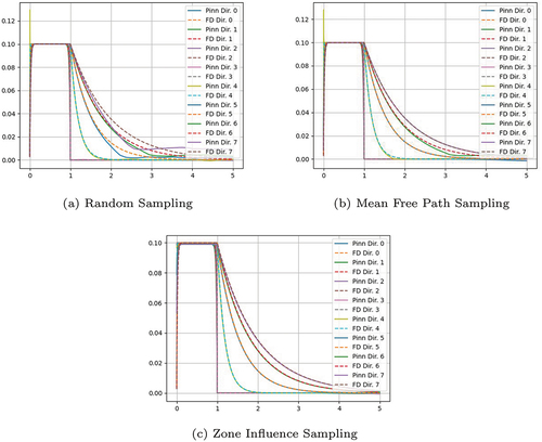
The results of this sampling technique are shown in Fig. 10b, where improvement is evident in the optically thin region. However, some error is still noticeable. To reduce it, we take into account the relative influence caused by an error in the different regions of the problem. For example, an error in the optically thick ($x\in [0,1]$) region would contribute roughly 50 times more to the loss than the same error in the optically thin region would. To counteract this, we sample more heavily in the optically thin region, so the residuals are both able to be reduced at the same rate, as described in Sec. III.F. The results of the zone-influence sampling are shown in Fig. 10c, where the aggregation of these sampling heuristics is used, leading to good agreement between the PiNNs and the FD solutions.

IV.D. Problem 4

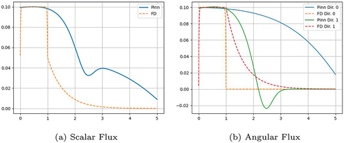
This problem is one of the more difficult to represent with a neural network due to the large void present on the right side of the domain. The void in this problem differs from the void in Problem 5 due to the length of the void region compared to the nonvoid one being much larger in this problem. The extent of each spatial zone and the material properties are given in Table IV. The scalar flux of the PiNN solution and FD solution are shown in Fig. 11. In this problem, the angular direction that starts in the void region should stay at zero for a long length before entering the region with a source on the left side of the domain. As there is no source or absorber in the void region, the residual in this void region is merely given by the streaming term. Hence, training errors propagate downstream from right to left before entering the absorber and source region on the left side of the domain. Additionally, since the error in this left side of the domain is nonzero due to the source and absorber in that region, the streaming error in the void region is approximately neglected in the training residual of the neural network. This causes a poor representation of the neutron flux in the void part of the domain.

TABLE IV Problem 4 Definition

$x$	${\mathrm{\Sigma }}_a$	${\mathrm{\Sigma }}_s$	$q$
[0,1]	50	0	5
[1,5]	0	0	0

Fig. 11. Scalar flux Problem 4: PiNN and FD solutions.

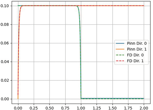
In order to demonstrate that the length of void is what makes this problem challenging to learn and causes error buildup due to streaming, we present the results of a modified problem with a reduced length of void. The modified problem is described in Table V. The angular flux of the PiNN solution and FD solution are shown in Fig. 12. In this graph, there is good agreement between the solutions leading credence to the hypothesis that the large region of void is what causes the failure of the PiNN in the unmodified Problem 4.

TABLE V Problem 4’ Definition

$x$	${\mathrm{\Sigma }}_a$	${\mathrm{\Sigma }}_s$	$q$
[0,1]	50	0	5
[1,2]	0	0	0

Fig. 12. Angular flux Problem 4’: PiNN and FD solutions.

IV.E. Problem 5

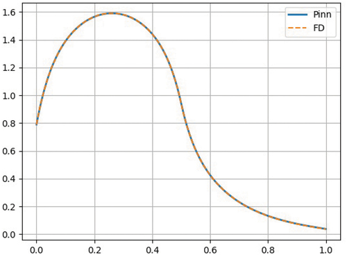
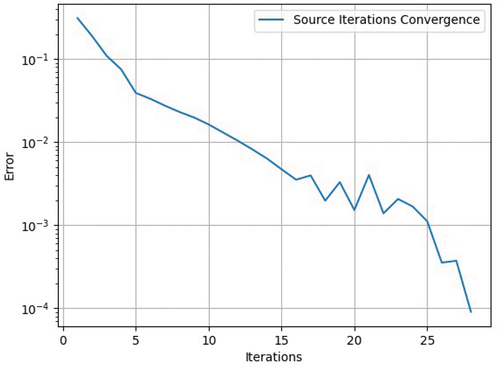
This heterogeneous problem is a fairly standard benchmark for 1-D transport solvers. A description of the problem is given in Table VI. The results of the PiNNs compared to the results of a FD solution are shown in Fig. 13. There is good agreement between these two solutions. This problem again proves that our PiNN implementation, with Fourier Features, wrapped inside a SI, leads to very good agreement when compared to a fine-mesh FD solution. In Fig. 14, we present the SI error. This error was calculated by the L-2 relative error between the new and old scalar fluxes.

TABLE VI Reed’s Problem Definition (Problem 5)

$x$	${\mathrm{\Sigma }}_a$	${\mathrm{\Sigma }}_s$	$q$
[0,2]	50	0	50
[2,3]	5	0	0
[3,5]	0	0	0
[5,6]	0.1	0.9	1
[6,8]	0.1	0.9	0

Fig. 13. Scalar flux Problem 5: PiNN and FD solutions.

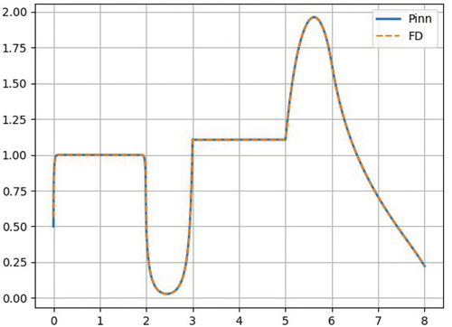
Fig. 14. Source iteration convergence error Problem 5.

V. CONCLUSIONS

In this paper, we described and employed PiNNs to solve the radiation transport equation. PiNNs are a type of neural network that uses the residual of a governing equation to train without requiring pregenerated training data. We applied PiNNs to transport problems in heterogeneous 1-D slabs. The standard SI technique was wrapped around the training of the PiNN. We observed that PiNNs can yield poor solutions in heterogeneous problems, and we showed how Fourier Features and improved point-sampling methods can lead to better PiNN performance in those problems. Fourier Features generally improve the PiNN accuracy for heterogeneous problems, and the sampling methods further increased this performance at material interfaces and in problems with very different material properties.

There is a large amount of potential future research into PiNNs applied to radiation transport. First, the integration of scattering into the residual could allow for only a single PiNN to simulate an entire problem with direction as an input. Second, the PiNN algorithm should be tested for radiation problems in higher spatial dimensions. Third, another unique application of this PiNN algorithm is having multiple angular quadratures for a single problem. This is not possible with traditional numerical methods, but PiNNs could be adapted fairly seamlessly such that different spatial regions of the problem have varying levels of angular requirement. Fourth, an investigation into parameterized PiNNs, where material properties become additional inputs to the neural network, would be beneficial. This could reduce the issue of the large computational cost associated with training a PiNN by making the trained PiNN able to very quickly solve a wide range of problems. Fifth, the last potential area of research for PiNNs applied to radiation transport is enforcing causality during training (see, for instance, Ref. 11); this is of interest for radiation transport due to its similarity with the transport-sweep solution technique used in traditional $S^N$ transport solvers.

Disclosure Statement

No potential conflict of interest was reported by the author(s).

Additional information

Funding

This work was performed under the auspices of the U.S. Department of Energy. Lawrence Livermore National Laboratory is operated by Lawrence Livermore National Security, LLC, for the U.S. Department of Energy, National Nuclear Security Administration under Contract DE-AC52-07NA27344. This research was funded by LLNS under research subcontract B640889.

References

- O. SIMEONE, “A Brief Introduction to Machine Learning for Engineers”; https://arxiv.org/abs/1709.02840 (2017).
- A. LINDHOLM et al., Machine Learning: A First Course for Engineers and Scientists, Cambridge University Press (2022).
- G. E. KARNIADAKIS et al., “Physics-Informed Machine Learning,” Nat. Rev. Phys., 3, 422 (2021).
- J. I. C. VERMAAK et al., “Massively Parallel Transport Sweeps on Meshes with Cyclic Dependencies,” J. Comput. Phys., 425, 109892 (2021); https://doi.org/10.1016/j.jcp.2020.109892.
- M. RAISSI, P. PERDIKARIS, and G. E. KARNIADAKIS, “Physics-Informed Neural Networks: A Deep Learning Framework for Solving Forward and Inverse Problems Involving Nonlinear Partial Differential Equations,” J. Comput. Phys., 378, 686 (2019); https://doi.org/10.1016/j.jcp.2018.10.045.
- D. P. KINGMA and J. BA, “Adam: A Method for Stochastic Optimization”; https://arxiv.org/abs/1412.6980 (2015).
- D. C. LIU and J. NOCEDAL, “On the Limited Memory BFGS Method for Large Scale Optimization,” Math. Program., 45, 503 (1989); https://doi.org/10.1007/BF01589116.
- S. WANG, X. YU, and P. PERDIKARIS, “When and Why PINNs Fail to Train: A Neural Tangent Kernel Perspective,” J. Comput. Phys., 449, 110768 (2022); https://doi.org/10.1016/j.jcp.2021.110768.
- S. WANG, H. WANG, and P. PERDIKARIS, “On the Eigenvector Bias of Fourier Feature Networks: From Regression to Solving Multi-Scale PDEs with Physics-Informed Neural Networks,” Comput. Methods Appl. Mech. Eng., 384, 113938 (2021); https://doi.org/10.1016/j.cma.2021.113938.
- M. TANCIK et al., “Fourier Features Let Networks Learn High Frequency Functions in Low Dimensional Domains”; https://arxiv.org/abs/2006.10739 (2020).
- S. WANG, S. SANKARAN, and P. PERDIKARIS, “Respecting Causality Is All You Need for Training Physics-Informed Neural Networks”; https://arxiv.org/abs/2203.07404 (2022).
- A. DAW et al., “Mitigating Propagation Failures in PINNs Using Evolutionary Sampling”; https://arxiv.org/abs/2207.02338 (2022).
- R. MOJGANI, M. BALAJEWICZ, and P. HASSANZADEH, “Lagrangian PINNs: A Causality-Conforming Solution to Failure Modes of Physics-Informed Neural Networks”; https://arxiv.org/abs/2205.02902 (2022).
- E. E. LEWIS and W. F. MILLER, Computational Methods of Neutron Transport, p. 1, Wiley (1984).
- T. R. HILL, “ONETRAN: A Discrete Ordinates Finite Element Code for the Solution of the One-Dimensional Multigroup Transport Equation,” LA-5990-MS, p. 6, Los Alamos National Laboratory (1975).
- T. A. WAREING et al., “Discontinuous Finite Element SN Methods on Three-Dimensional Unstructured Grids,” Nucl. Sci. Eng., 138, 3, 256 (2001); https://doi.org/10.13182/NSE138-256.
- M. W. HACKEMACK and J. C. RAGUSA, “Quadratic Serendipity Discontinuous Finite Element Discretization for Sn Transport on Arbitrary Polygonal Grids,” J. Comput. Phys., 374, 188 (2018); https://doi.org/10.1016/j.jcp.2018.05.032.
- A. G. BAYDIN et al., “Automatic Differentiation in Machine Learning: A Survey,” J. Mach. Learn. Res., 18, 1 (2018).
- M. M. POZULP et al., “Heterogeneity, Hyperparameters, and GPUs: Towards Useful Transport Calculations Using Neural Networks,” LLNL-PROC-819671, Lawrence Livermore National Laboratory (2021).
- W. H. REED, “New Difference Schemes for the Neutron Transport Equation,” Nucl. Sci. Eng., 46, 2, 309 (1971); https://doi.org/10.13182/NSE46-309.
- T. G. GROSSMANN et al., “Can physics-informed neural networks beat the finite element method?” arXiv.2302.04107, 2023.