?Mathematical formulae have been encoded as MathML and are displayed in this HTML version using MathJax in order to improve their display. Uncheck the box to turn MathJax off. This feature requires Javascript. Click on a formula to zoom.
Abstract
A new method for directly sampling the resonance upscattering effect is presented. Alternatives have relied on inefficient rejection sampling techniques or large tabular storage of relative velocities. None of these approaches, which require pointwise energy data, are particularly well suited to the windowed multipole cross-section representation. The new method, called multipole analytic resonance scattering, overcomes these limitations by inverse transform sampling from the target relative velocity distribution where the cross section is expressed in the multipole formalism. The closed-form relative speed distribution contains a novel special function we deem the incomplete Faddeeva function, and we present the first results on its efficient numerical evaluation.
Keywords:
I. INTRODUCTION
Early continuous-energy Monte Carlo neutron transport programs sampled scattering from nuclei in thermal motion assuming that the scattering cross section is effectively constant within the scattering kernel.[Citation1] However, as Refs. [Citation2,Citation3] detail, the resulting scattering kernel implied by the constant cross-section approximation may be far from the actual double-differential cross section near a scattering resonance. As shown in Refs. [Citation4,Citation5], the resulting error tends to cause a worst-case 11% underestimation of the Doppler feedback coefficient in a pressurized water reactor (PWR), with even larger discrepancies in high-temperature gas-cooled reactor problems.
As exhibited by the Power Reactor Analysis using GPU-based Monte Carlo Algorithm (PRAGMA) project,[Citation6,Citation7] the conventional methods for treating this effect leave something to be desired on graphics processing unit (GPU) architectures, which constitute the majority of computational power on most leading supercomputers. Due to the unique architecture of the GPU, algorithmic modifications to standard Monte Carlo algorithms for neutron tracking can tangibly accelerate computation.[Citation7] In the same direction, we herein present a GPU-friendly method for handling resonance upscattering when the windowed multipole (WMP)[Citation8] formalism is employed to represent cross sections. In particular, the heuristic for fast GPU code is to avoid rejection sampling and accesses to distantly spaced places in memory, which the new method achieves. To give context to the new method, we first recall some of the conventional methods for modeling resonance upscattering.
The Doppler Broadening Rejection Correction (DBRC)[Citation9] was one of the early proposed techniques to treat the effect of strong variations of the interaction cross section within the energetic vicinity of a scattering neutron, whereas tables had been used prior.[Citation10] The method has since been implemented in numerous continuous-energy Monte Carlo neutron transport programs[Citation9,Citation11–13] and has been shown to successfully model the resonance upscattering effect. However, DBRC suffers from rejection probabilities as high as 99.995%[Citation14] for neutron energies in the vicinity of a resonance.
The weight correction method (WCM)[Citation4] also successfully models the effect of resonances on the double-differential cross section of nuclei in thermal motion. This method adjusts the weight of particles to provide numerically correct results even when the constant cross-section double-differential free gas distribution is employed. WCM carries the same benefit as our newly proposed method of not requiring an additional rejection loop or tables; however, adjustments to the particle weights introduce substantial variance to the overall Monte Carlo simulation, thus degrading estimates on quantities of interest.[Citation6]
Another technique known as target motion sampling[Citation15] can be used to model the resonance upscattering effect. However, this method is only applicable to Monte Carlo neutron transport programs employing the delta tracking technique. Unfortunately, the performance of delta tracking appears to be lackluster on GPUs.[Citation16]
The relative velocity sampling (RVS) method[Citation14,Citation17] was created to ameliorate the high rejection rates characteristic of the rejection algorithms used to model resonance upscattering. These schemes, in essence, sample probability distributions proportional to , where
is a distribution and
. One then samples from
and accepts the sample with probability
. The RVS method moves the direct sampling from the thermal motion term to the cross-section term, thus worsening the average case rejection rate but massively improving the worst-case rejection rate.
The relative speed tabulation (RST) method[Citation6] was developed to address the rejection sampling performance impact on GPUs. RST is the first resonance upscattering modeling technique not requiring a rejection loop or bivariate scattering distribution tables. The key observation underlying RST is that the target velocity distribution can be factorized into a marginal relative speed distribution encapsulating the information about the resonances and a simple distribution of the target polar angle conditioned on the target relative speed. Consequently, the univariate relative speed cumulative distribution function (CDF) can be tabulated in select areas of the pointwise cross section, and the conditional polar angle distribution is then directly sampled without requiring any additional data or rejection step.
Despite its simplicity and efficacy on GPUs, the RST method comes with some clear disadvantages. Gigabytes of additional memory are used to store the relative speed CDFs at each energy point and temperature on a pointwise cross-section representation if all nuclides have the resonance upscattering effect treated. The resonance influence on the double-differential cross section is thus restricted for practical reasons to a select few nuclides in the problem to avoid extreme memory usage. Moreover, the method introduces some discretization errors in temperature, although this has been shown to be a reasonable approximation.
If one could avoid pretabulated relative speed distributions, this could substantially reduce the memory needs and avoid costly divergent memory accesses. Reducing serialized memory accesses on GPUs typically leads to significant speedups.
We propose a new method that does just that, and achieves this using the WMP cross-section representation.[Citation8] Our new method introduces a novel special function we have deemed the incomplete Faddeeva function, which encodes the behavior of the temperature-dependent influence of resonances on the double-differential scattering distribution. It relies on the numerical inversion of the analytic representation of the relative speed distribution under the WMP formalism and polar angle sampling in the same manner as the RST method, but without any precomputed tables.
This contrasts the WMP-based target velocity sampling technique presented in Ref. [Citation18], which is similar in nature to the newly presented method in this work. However, the method in Ref. [Citation18] relies on the separation of the target velocity distribution into a zero-kelvin cross-section component and a Maxwell-Boltzmann component. This method thus requires a numerical inversion step of the integrated scattering cross-section function wrapped in a rejection loop, similar to Ref. [Citation14], but instead using a functional representation of the integrated cross section rather than tabular.
The algorithm presented in Ref. [Citation19] shows how the relative speed can be sampled in the WMP framework similarly to our work. However, Ref. [Citation19] relies on fitting a sum of Gaussian to replace the multipole expansion, thus representing the zero-kelvin scattering cross section in the form
While it remains to be seen that Gaussians can be used to approximate all poles appearing in a WMP library, this proposed approximation introduces a considerable number of degrees of freedom to the problem, with 18 unknowns for each pole. The optimization problem thus encountered is highly nonlinear and nonconvex, leading to fitting difficulties. Additionally, scattering kernels in the formalism in Ref. [Citation19] cannot be straightforwardly differentiated with respect to WMP parameters, which would be needed to perform sensitivity analyses.
Our new method, multipole analytic resonance scattering (MARS), only requires the same WMP data as would be used in a calculation without any treatment of the resonance upscattering effect, thus avoiding the need for additional tables or fitting steps. We demonstrate the new method’s negligible performance overhead compared to other methods for sampling the resonance upscattering effect on CPU architectures, with future work exploring its optimized implementation on GPUs.
II. THEORY
Rothenstein and Dagan[Citation2] expound on the rigorous Doppler-broadened double-differential cross section. Since the exact expression for the lab frame scattering distribution is quite complicated, authors presenting algorithms to model it typically choose to forgo the lab frame expression and instead reason in terms of joint distributions of the target velocity and direction cosine relative to the direction of projectile motion. After sampling the target speed and direction cosine, standard two-body collision kinematics for elastic scattering are employed, where the center of the mass angular distribution comes from the nuclear data file. The resulting physics matches the complicated expressions of Ref. [Citation2].
Similarly, considering the distribution of collision target velocities, this joint distribution is
where is the Maxwell-Boltzmann distribution of target speeds
the variable with units of inverse velocity parameterizes the target velocities, and the distribution
is a uniform distribution between −1 and 1. The other variables are
, the distribution’s normalizing constant;
, the relative speed of the neutron with respect to the target;
, the zero-kelvin scattering cross section;
, the target mass;
, the Boltzmann constant;
, the absolute temperature; and
, the target speed.
Classically, the approximation that is constant has been employed. However, it was shown in Refs. [Citation3,Citation4] that this approximation is incorrect in the vicinity of resonances, where
varies over a few orders of magnitude, preferentially causing scattering with targets of relative velocity more closely matching the scattering resonance peaks. The various aforementioned techniques are all just methods for sampling from the distribution of EquationEq. (2)
(2)
(2) with arbitrary forms of the function
.
More specific knowledge about the form of can be employed. It has been shown extensively[Citation20,Citation21] at this point that the cross section is accurately represented as a sum of poles in addition to a low-order Laurent expansion
, namely,
In fact, for the purposes of sampling the resonance upscattering effect, we claim and later numerically demonstrate that the narrow range of attainable leads the zero-kelvin cross section to be accurately represented as a single pole and a linear term over a sufficiently narrow range of energies:
The and
terms are calculated through a linearization process to avoid some complexities with higher-order polynomial fitting. An algorithm for finding the best values of
and
is presented in Sec. II.D.
With this approximation, we use the technique developed in Ref. [Citation6]. Rather than attempting to sample the target speed and direction cosine
, one instead samples first the relative velocity
, and then samples
from the distribution of
conditioned on
. The distribution in this form for projectile speed
is thus[Citation6]
Next, as previously shown for the Doppler-broadening of the WMP format[Citation8] and the original full multipole format,[Citation22] we note the term to be negligible and use the following:
At this point, we write the multipole cross section in terms of the relative velocity rather than in terms of energy. The formula to use is
If we define the auxiliary variables and
, and insert EquationEq. (8)
(8)
(8) into the marginal target collision rate distribution in terms of relative speed [EquationEq. (7)
(7)
(7) ], some algebra reveals that
where , which represents a dimensionless measure of the energy gap between the center of the Maxwell-Boltzmann distribution and the location of the resonance.
At this point, we can consider the CDF for the random variable (dimensionless target velocity) conditioned on
(dimensionless projectile velocity). Integrating EquationEq. (9)
(9)
(9) yields
where is the normalizing constant. After distributing the integral and interchanging the
operator with integration, we obtain
where the normalizing constant for the distribution is
which we point out is nothing more than the Doppler-broadened scattering cross section at temperature under the single pole approximation.
The new special function we deem the incomplete Faddeeva function is defined as
It can easily be seen that , as per the definition of the Faddeeva function for
:
Indeed, for this application, and we maintain this assumption going forward. A specialized root finder has been developed to quickly invert this CDF and consequently sample the relative velocity. This thus constitutes a method to sample target velocities without rejection sampling or extensive tables.
The novelty in our approach lies entirely in the treatment of the zero-kelvin cross section and analytical representation of the relative speed CDF. After sampling from the relative speed distribution, we must sample the target polar angle distribution conditioned on the relative speed, as done in Ref. [Citation6]. For completeness, we conclude with the CDF of the target speed
for which Ref. [Citation6] provides a straightforward sampling technique. The remaining work is purely numerical, particularly in requiring an efficient, reasonably accurate algorithm for the incomplete Faddeeva function .
II.A. Incomplete Faddeeva Function
The forthcoming discussion explores the properties of the incomplete Faddeeva function, with a particular focus on properties that can be leveraged to obtain efficient numerical approximations to it. We advise the reader that absorbing this section in depth is not necessary to grasp the claims and algorithms made herein.
The incomplete Faddeeva function, as defined by EquationEq. (13)(13)
(13) is
. This section attempts to build some intuition as to how this function behaves as
and
individually vary. In resonance upscattering treatment,
parametrizes the location, height, and width of the resonance with respect to the Maxwell-Boltzmann distributed velocities. Values of
correspond to scattering resonances exactly situated at the mean component of relative speed along the neutron’s line of flight predicted by the Maxwell-Boltzmann distribution. Values of
correspond to resonances at higher energies than the particle’s energy, and therefore induce preferential scattering with relative velocities higher than the incident velocity, and vice-versa for
.
parametrizes the dimensionless target relative speed. Small values of
imply tall, narrow resonances, with a limit of
being a singularity representing a resonance of infinite cross section. Large values of
model wider, weaker resonances.
plots the incomplete Faddeeva function as a function of for a few values of
, and shows the behavior of its real part in
for a few values of
. Both illustrate the rapidly varying behavior of this function for small values of
when
, where a sharp peak follows the value of
near the real line. particularly shows the approach to the familiarly shaped
as
. The figures also show that
is an increasing function in
, as would be expected of a CDF. This behavior is explained by the following asymptotic analysis.
Fig. 1. for a few values of
. The height represents the magnitude and the coloring is done by phase.
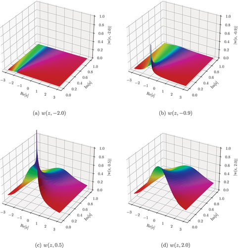
Fig. 2. for a few values of
. The legend is the imaginary number added to the real part specified in each figure’s caption. The plotted quantity is normalized by
so all lines tend to unity as
grows.
![Fig. 2. ℜ[w(z,x)] for a few values of z. The legend is the imaginary number added to the real part specified in each figure’s caption. The plotted quantity is normalized by ℜ[w(z)] so all lines tend to unity as x grows.](/cms/asset/913b823d-3554-4c18-91f1-769c32a45a9f/unse_a_2204810_f0002_oc.jpg)
Humliĉek[Citation23] provides the following asymptotic formula for the Faddeeva function without derivation:
Considering the definition of the Faddeeva function once more in EquationEq. (14)(14)
(14) , this approximation results from supposing that if
is large, and that only values of
near zero contribute to the integral, we can approximate
as
which immediately yields the asymptotic estimate of EquationEq. (16)(16)
(16) . Proceeding with the same approximation in the context of the incomplete Faddeeva function, we thus obtain
suggesting a close connection between the incomplete Faddeeva function’s behavior in and the error function. In fact, this hunch is confirmed by the following identity, which connects the incomplete Faddeeva to the standard Faddeeva function:
Proof of this relation is provided in Appendix A.
An even more accurate asymptotic estimate can be obtained for large , approximating the pole term as
This matches the value, slope, and curvature with respect to of the pole about
. Substituting this back to EquationEq. (13)
(13)
(13) and adjusting the expression such that
is strictly increasing [as suggested by EquationEq. (18)
(18)
(18) ], and matching the asymptotic value of
as suggested by EquationEq. (19)
(19)
(19) , results in
EquationEquation (21)(21)
(21) is sufficiently accurate to be used in practical computations, as shown by .
Fig. 3. Accuracy of the approximation for
. An unshifted error function is shown for comparison, representing a more naive asymptotic approximation to
.
![Fig. 3. Accuracy of the w(z,x) approximation for |ℜ[z]|>5. An unshifted error function is shown for comparison, representing a more naive asymptotic approximation to w(z,x).](/cms/asset/b467b9cb-f91f-4f90-af0b-28cfd08e9915/unse_a_2204810_f0003_b.gif)
In the context of resonance scattering, EquationEq. (21)(21)
(21) shows that the relative speed distribution gets shifted forward by a nondimensionalized factor of
with its influence scaling by
times the resonance’s residue, as suggested by EquationEq. (11)
(11)
(11) .
Another useful property of the incomplete Faddeeva function is a simple connection between its derivative in the complex plane and its value. This is similar in nature to the derivative of the Faddeeva function[Citation24]:
The relation we have obtained generalizes this as
which clearly maintains consistency with EquationEq. (22)(22)
(22) as
. This fairly simple connection between the derivative of
and its value can be utilized for efficient sensitivity analyses of the scattering kernel with respect to WMP parameters.
The forthcoming discussion presents some further concepts in the direction of the efficient numerical evaluation of the incomplete Faddeeva function. Going forward, we denote the second integral appearing in EquationEq. (19)(19)
(19) as
where . While it may seem that a half-range Gauss-Hermite quadrature might work well to efficiently approximate EquationEq. (24
(24)
(24) ), this is not the case. First, complex exponentials would have to be calculated at each quadrature point. Second, as the real part of
grows, the integrand oscillates more. In practice, values of
are frequently encountered, and low-degree quadratures would not capture the oscillation. Additionally, given that the value of
is small, the denominator becomes nearly singular when
. In fact, when
,
becomes a discontinuous function in
when interpreted as a principal value integral.
EquationEquation (24)(24)
(24) is equivalent to the incomplete Goodwin-Staton integral, referred to in Ref. [Citation25]. However, to our knowledge, only asymptotic analysis has been performed on this type of integral before, without any development of numerical routines. Recent work in the field of finance[Citation26] presents results for computing what the authors define as the extended incomplete Goodwin-Staton integral, for which the
case is of interest in the present discussion. Unfortunately, the authors’ numerical method works for all cases except
, suggesting EquationEq. (24)
(24)
(24) to be of a fundamentally different nature.
In our experience, the difficulty with large cannot be ameliorated by a stationary phase technique,[Citation27] as these tend to accentuate the pole behavior and remain of similar difficulty for half-range Gauss-Hermite quadratures.
In the WMP method, is near zero, as shown in . Therefore, we can expect to frequently encounter nearly singular integrands in EquationEq. (24)
(24)
(24) . An efficient numerical technique that explicitly treats this behavior can be devised by first noticing that
satisfies this differential equation in the complex plane
Fig. 4. Distribution of the imaginary part of the poles in the WMP method. These were collected from every nuclide in the OpenMC regression testing data set based on ENDFVII.1.
This can be used to connect the value at a point
to another point
. The integrating factor technique shows that
If the distance between and
is small, the exponential in the numerator of EquationEq. (26)
(26)
(26) can be Taylor expanded about
to yield an efficient numerical scheme.
We have found that the imaginary part of can be calculated with a closed-form, discontinuous-in-
formula. Because the nearly discontinuous behavior of
in
is the main source of difficulty here, EquationEq. (26)
(26)
(26) can be used to resolve this behavior accurately after calculating the value of
. The real part of
is continuous in
but is not available in terms of elementary functions; however, it is readily amenable to numerical approximation. In conclusion, the real and imaginary part of
contrast with each other: the former is readily numerically approximated by series or similar methods, whereas the latter is discontinuous and therefore not amenable to series or rational function approximation, and fortunately has an exact formula.
The first goal at hand is to calculate for real values of
. This can be written as
The linearity of integration can be distributed over both trigonometric terms. Each of the resulting integrals can be found as respective sine and cosine transform integrals, which are listed in Ref. [Citation28]. Combining the results from the sine and cosine transform tables yields
Next, we can find an approximation for the real part of :
This expression can neither be written in terms of elementary nor special functions to our knowledge. In order to manipulate it to obtain a numerical expression, consider the auxiliary function
which again, of course, cannot be represented in terms of elementary or special functions. This pinpoints the difficulty in calculating the real part of because
We thus seek a straightforwardly differentiable approximation to . The intuition behind our forthcoming numerical approximation to
comes from the fact that for
,
is negligible in the denominator compared to
over the range where the
weighting is large, hence
Where is the Dawson F function.[Citation24] By standard asymptotic analysis, matching the
derivative at
and the
asymptote for the Dawson F function results in the improved estimate
which is accurate to within about 5% across the full range of values. However, this level of accuracy is not appropriate for engineering calculations.
To build more intuition for , its close relation to the Dawson F function is evinced by considering the Maclaurin series in
for both
and
which further highlight the utility of maintaining the consistency of with its asymptotic sister
. The series are the same, but with the addition of the exponential integral multiplying factors in
.
In order to find such a numerical relation that maintains this consistency in the asymptotic case, EquationEq. (30)(30)
(30) can be transformed via the interchange of differentiation and integration. Consider the generalized function
Differentiating reveals that
The fundamental theorem of calculus then applies:
Using the fact that and doing a change of variables, EquationEq. (30)
(30)
(30) becomes
which confirms our hunch about the close relation of to
; it is an infinite superposition of stretched and scaled Dawson F functions.
We have found success in inserting an approximation for into EquationEq. (39)
(39)
(39) . Well-known approximations to
based on rational expressions and other elementary functions[Citation29,Citation30] do not result in numerically useful expressions. However, noting that
it can be seen that approximations to in the form of a power series can be computationally efficient in light of the recursion relation for exponential integrals:
Careful attention must be paid to the floating point properties of this relation.[Citation31] The magnification of computational errors grows arbitrarily large, and we later present a specialized numerical algorithm guaranteeing floating point stability.
In order to thus obtain a simple, efficient approximation to , we employ the Chebyshev expansion valid for
presented in Ref. [Citation32]. The results of our method could be improved by using a finer piecewise division for the Chebyshev expansion of
as in Ref. [Citation33], but we have used the present approach for simplicity of implementation. Thus, if the truncated Chebyshev expansion of
is converted to the power series basis
we obtain approximations of the form
III. NUMERICAL IMPLEMENTATION
III.A. Stable, Efficient Calculation of an  Sequence
The magnification of error in the forward recurrence relation for exponential integrals from Ref. [Citation31] is
Notably, the error magnification of the reverse recurrence relation is the reciprocal of this quantity. Moreover, is a function increasing from 1, reaching a maximum and monotonically descending below 1.[Citation31] As a consequence, a critical index
exists such that iterating outward from it results in a numerically stable recursion algorithm. In terms of evaluating EquationEq. (43)
(43)
(43) , this means splitting the polynomial in
into parts above the index
and those below. After computing
, Horner’s method is used in the reverse recurring relation down to the term of order
, and forward recursion is employed to evaluate the polynomial of degree leading from
up to
.
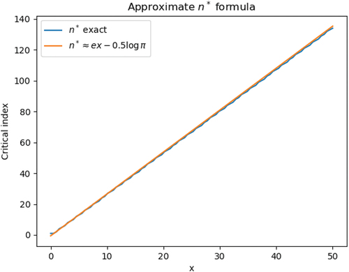
A simple result we have obtained is that the smallest value of , such that
is well approximated by
Appendix B shows how this can be obtained. illustrates the accuracy of EquationEq. (46)(46)
(46) . Using this information, explicitly states the procedure to calculate
and its derivative with respect to
. While the use of a power-basis polynomial is suboptimal, numerically speaking, the main source of numerical error in this scenario originates from the recursive exponential integral formula. The specification of the algorithm assumes that an accurate method for computing
has been provided, which is well documented in many other works. We have employed a C++ adaptation of the continued fraction approximation employed by the Cephes library,[Citation34] which is documented in Ref. [Citation24].
Fig. 5. Approximate solution to finding the first value of such that
.
Table
III.A.1. Jump Integral
After computing the value of , the differential equation of EquationEq. (25)
(25)
(25) , which
follows, can be used to calculate
. We calculate
in this manner due to the nearly discontinuous behavior of
; it has a jump discontinuity about
if
. Because the imaginary part of
is small in WMP libraries, the resulting behavior is nearly discontinuous, and hence is not captured efficiently by general approximation techniques; finely resolved tables or high polynomial orders would be required. Our approach thus resolves the discontinuous component exactly with the piecewise function [EquationEq. (28)
(28)
(28) ]. The nontrivial part of EquationEq. (26)
(26)
(26) is the transcendental integral
We have deemed this term the jump integral because it allows for jumping from values of on the real line to values above the real line in the complex plane. While it seems that our issue of approximating the transcendental integral
has seemingly not been heretofore ameliorated due to the appearance of yet another transcendental integral [EquationEq. (47)
(47)
(47) ], a change of variables puts it into a form suitable for numerical approximation,
where again, . Because
is small as, shown by , the argument to the exponential term is similarly small. Where this integral is well defined (
), the exponential term can be expanded in its Maclaurin series and integrated term by term
It is verified that the coefficients satisfy the two-term recurrence
Next, the term-by-term integrals appear in the form
where is the incomplete beta function, defined as
A recursion formula derived as a special case of formulas in Ref. [Citation24] efficiently calculates these incomplete beta function values of higher in sequence:
In combination with the fact that
this yields an efficient numerical scheme for evaluating an integral of the truncated Maclaurin series of the exponential of EquationEq. (48)(48)
(48) .
details the combination of all of these facts for an efficient approximation to . This approximation works very well for problems with
, which easily covers the range of scattering events where resonances appreciably affect the double differential at temperature. Outside of that range, the integral becomes increasingly oscillatory, so an asymptotic approximation is employed for
. This approximation is documented in Appendix D.
Table
Last, gives the overall algorithm to compute efficiently. It relies on access to some implementation of calculating
, e.g., the Johnson’s permissively licensed library,[Citation35] which implements a variety of approximations to achieve high accuracy, or one of the various rational approximations[Citation23,Citation36,Citation37] when higher error is permitted. Regardless of the chosen
implementation, our algorithm maintains asymptotic consistency such that
. This work leverages a recent approximation tailored for WMP.[Citation38]
Table
III.B. Pole Sampling Approximation
A key approximation of our technique that enables its computational efficiency is viewing the multipole cross section in the relative speed distribution as a mixture distribution. The theoretical justification is that if poles are present and sufficiently close to the incident neutron energy ( specifically), the relative speed probability density function (PDF) is well approximated by ignoring the polynomial contribution
This expression is not employed to actually sample the scattering distribution. Rather, it is best viewed as a mixture distribution in which each pole contributes a probability proportional to
which defines a discrete distribution. In order to avoid the need for auxiliary storage and the calculation of a normalizing constant to this distribution, we recommend finding the maximum of , where
are uniform random numbers differing for each pole. The
corresponding to the maximum of this expression follows the desired discrete distribution. We also note that the quantity
is exactly the Doppler-broadened contribution to the integrated scattering cross section, so this sampling procedure incurs no additional Faddeeva function evaluation overhead if this is done in tandem with a WMP cross-section lookup operation.
Finally, we emphasize that the pole sampling approximation is not precisely consistent with the original multipole cross-section representation. Instead, it uses the fact that polynomial contributions to the cross section negligibly affect the scattering kernel, while poles do so substantially.
III.C. Finding the Values of and
While it may seem that the polynomial contribution to EquationEq. (5)(5)
(5) could come as the first terms from the polynomials defined within the windows, as Ref. [Citation19] used, we have found in practice that this choice is inconsistent with the approximation of the pole sampling technique and leads to negative cross-section values.
To remedy this issue, we use the heuristic that the relative error of the cross section local approximation is minimized by matching polynomial values in the vicinity of the dip of the resonance. The location of the scattering resonance trough is calculated as
where
At this point, the window index of is calculated.Footnotea
This may be a different window from the incident neutron energy’s window. The WMP cross section of EquationEq. (4)
(4)
(4) is then evaluated at
but excluding the sampled pole
, i.e.,
From there, is calculated at the same point, this time only including contributions from the polynomial expansion but not from any poles. This linearization technique has been found to improve the accuracy of our method when considering nuclides with tightly spaced resonances such as 235U. For complete clarity, the resulting expression is
Finally, a linearization of the cross section in space has been obtained. For use with the root finder, the nondimensional variable
is preferable, so
is appropriately shifted and
appropriately scaled.
III.D. Inverting the Relative Speed CDF
To sample from the relative speed PDF, we employ the CDF inversion technique. A naive attempt at this would be a few bisection root-finding steps followed by a handful of Newton-like iterations. In practice, we have found that five bisection iterations followed by three Halley-Newton iterations resolves the root to within an acceptable tolerance; however, a far more efficient root finder has been developed that takes a maximum of four iterations total, only requiring more work for unusual edge cases.
The bootstrapping step, as we call it, is essential to an efficient implementation of MARS. The bootstrapping step cheaply obtains an initial guess to the solution of the CDF inversion problem, from which a small number of Newton-like iterations improve the solution.
The key to doing so lies in finding a cheap approximation to the inverse of the CDF with general pole parameters. In order to do so, we first move from the root-finding space of to the nonlinearly mapped variable
. The intuition behind using this modified space is that as the resonances become weak and the incident neutron energy becomes high, it can be shown that the CDF is simply equal to
, which ranges between zero and one. Resonances and low-energy free gas effects simply act as perturbations to this linear function, which enables a good starting point for approximating the root location.
The next step in improving the CDF model in the mapped space is to observe that the contribution of collision probability from the resonance largely does not depend on its imaginary part. Increasing the imaginary part of the resonance broadens it and decreases its height. Therefore, the magnitude of the jump in when
is near
quantifies the probability that the neutron experiences a collision near the peak of the resonance. The jump in
for small
about
is approximately
, and therefore the probability contribution due to the resonance is approximately
where is the normalizing constant given by EquationEq. (12)
(12)
(12) . Because this is an approximation, the probability of EquationEq. (65)
(65)
(65) may not be bounded between zero and one, so we threshold it to that range. In practice, the estimate provided here is accurate. We have found that this probability tends to be added into the CDF about
over the interval
. This estimate could obviously be tuned for greater accuracy.
One final tool we employ to bootstrap the root-finding process pertains to the values of the CDF about . In this case, numerous instances of functions occurring in its expression, such as
and
, take on easily calculated values. On top of that, the incomplete Faddeeva function has a closed-form expression when
of
Because is already computed and cached for the CDF inversion, the calculation of a complex exponential integral is the only difficulty. This is much easier and computationally cheaper to do than the more involved
evaluation, so any off-the-shelf approximation of
can be employed here.
Additionally, the derivatives of the CDF with respect to about
are also easily obtainable, which we use to further improve our root-finding guess. So far, we have only incorporated information from the first derivative, which has proven sufficient.
This leaves us with the following pieces of information from which the root estimate is extracted: the probability due to the resonance, its width, the value and slope of the CDF about , i.e.,
, and the known endpoint values of the CDF at 0 and 1. We therefore construct a function that is piecewise quadratic on the left and right of
. This quadratic interval ranges to either the endpoints
or
, or the resonance’s upper or lower range of probability gain, estimated here as x
. Note that this interval has to be mapped to an interval in
space. Because the interval of the resonance is small, the Jacobian of the transformation
, which is proportional to
(a quantity already computed), can be used to calculate the range in
space.
With this knowledge, the CDF can be approximated somewhat accurately in space. Despite the apparent complexity of what was just described, the inversion of the function in the previous paragraph can be done using simple branching logic, and at worst, the solution of a quadratic equation. Because translating the inverse of the previous function into code can take nontrivial effort, C++ code to achieve this has been provided in Appendix E. shows two examples of how this can be a quite satisfactory approximation of the CDF in
space when resonances are influencing the scattering distribution.
Fig. 6. The bootstrapping CDF provides a fairly accurate, easily invertible approximation to the true relative speed CDF to kickstart the root-finding process. The pairs of lines, moving from top to bottom, represent 35.25-eV, 36.25-eV, 38.25-eV, and 66.25-eV incident neutron energies.
IV. RESULTS
IV.A. Calculation of
In order to test the accuracy of Algorithm 3, we have computed reference values of using the scipy[Citation39] adaptive quadrature routine, scipy.integrate.quad, to evaluate the integral formulation [EquationEq. (13)
(13)
(13) ]. In the approximation of the jump integral [EquationEq. (47)
(47)
(47) ], only the first five terms in the series are retained. Where functions such as
or
appear, C++ standard library implementations have been employed. The implementation of
from Ref. [Citation35] has been employed. This results in the error profiles exhibited by , where we have plotted the real part of
). Because only the real part is of interest in resonance upscattering calculations, results on the error of the imaginary component are omitted.
Fig. 7. Error of for a few values of
. The legend is the imaginary number added to the real part specified in each figure’s caption. The plotted error
is normalized by
to match the scaling of . Where the scipy numerical integration routine returned NaNs, the lines disappear.
![Fig. 7. Error of ℜ[w(z,x)] for a few values of z. The legend is the imaginary number added to the real part specified in each figure’s caption. The plotted error wapprox(z,x)−w(z,x) is normalized by ℜ[w(z)] to match the scaling of Fig. 2. Where the scipy numerical integration routine returned NaNs, the lines disappear.](/cms/asset/e4f61aa3-6e1c-4836-869a-51ba96341ee9/unse_a_2204810_f0007_oc.jpg)
IV.B. Single Energy Testing
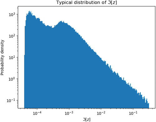
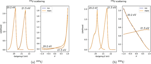
We first present in the relative speed distribution of 238U for two different energies and a few temperatures as calculated both by numerical integration and the MARS analytic CDF. The energies correspond to being in the trough and near the peak of a scattering resonance. These plots clearly show the influence of the resonances on the double-differential cross section; a nuclide with a constant cross section has a relative speed distribution that is very nearly an error function at epithermal energies. The relative speed distribution near resonances has a jumping effect that is governed by . They bear a resemblance to the
behavior depicted by .
Fig. 8. The MARS analytic CDF matches the numerically integrated relative speed CDFs. Some errors can be observed for the 1500-K case at 35.25 eV; scattering in the resonance dip is fortunately an extremely rare event.
If the relative speed distribution is correct, the resultant double-differential scattering distribution is also correct. shows this is the case for our method when compared to the RVS method of Ref. [Citation14]. These results were obtained from our modified version of OpenMC.Footnoteb It also shows that the pole sampling technique successfully works for 235U and its tightly spaced resonances.
Fig. 9. Scattering at 1200 K matches results from the RVS method well at two different energies. These energies interact with resonances for both nuclides.
IV.C. Pin Cell Reactivity Feedback
The 2.4%-enriched PWR pin cell example from the OpenMC suite of example problems was used to calculate Doppler reactivity feedback effects with four different models. The first and second used pointwise cross sections that were interpolated between 300 K, 600 K, 900 K, 1200 K, and 2500 K. The model was run at temperatures ranging from 300 to 1800 K in increments of 20 K. Of the two using pointwise cross sections, one used the historical constant cross-section (CXS) free gas scattering approximation and the second used the RVS method. The second two cases both used WMP cross sections, one using RVS and the second MARS. The ENDFB-VII.1 nuclear data set was employed. shows how these cases compare. Two hundred cycles with 10 inactive were employed, using 200 000 particles per cycle. The mean error of keff was thus converged to 20 pcm for each case.
Fig. 10. MARS matches the eigenvalue of the RVS method on a 2.4%-enriched fresh PWR pin cell problem. Line width represents estimated standard deviation of the mean.
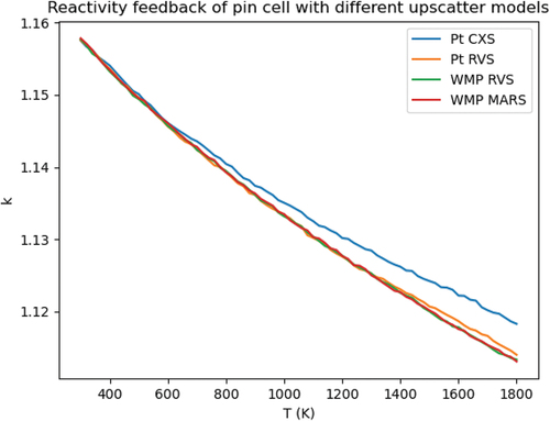
It can be seen that the pointwise cross-section representation incurs some interpolation error between 1200 and 1800 K. The MARS method matches the RVS results where multipole cross sections were employed. We can thus conclude that the new method works correctly across the range of energies where resonances influence the double-differential cross section at temperature for nuclides of both strong, distantly spaced resonances (238U) and closely spaced weak resonances (235U).
IV.D. Influence on Tracking Rate
Finally, in order to determine the computational efficiency of the new method, tracking rate comparisons were carried out on the same PWR pin cell example problem. The computational performance of both inactive and active cycles was assessed. For the active cycles, a 100 × 100 Cartesian mesh tallied flux, fission rates, and neutron production rates using track-length estimators. In addition, a spatially homogenized energy spectrum tally consisting of 500 equal-lethargy bins was applied.
An Intel Xeon W-2133 with six physical cores carried out the calculations and obtained the results depicted in . The results clearly demonstrate the computational efficiency of MARS compared to the RVS and DBRC methods. While it does not outperform RVS in this scenario, future work will explore its performance on vector computer architectures where we expect it to outperform.
TABLE I Tracking Rate Obtained by the Constant Cross-Section Treatment for Three Resonance Upscattering Models Showing MARS Is Comparable in Speed to Widely Accepted Techniques*
The computational expense incurred by tallying tends to render the performance impact of our new method particularly negligible. Collision estimators could be used on the mesh tally to improve the tracking rate, but we arbitrarily opted for track-length estimators. Due to subtle hardware-related effects, such as cache utilization or branch prediction, the tracking rates of the three resonance upscattering handling methods have different relative performances when comparing active and inactive cycles. Future work will explore detailed performance results on a variety of architectures.
V. CONCLUSION
Multipole formalism carries a variety of advantages compared to pointwise cross sections. Aside from its potential gains in computational efficiency on modern compute architectures, it enables accurate Doppler broadening without a library-size tradeoff,[Citation8] offers elegant sensitivity quantification, and narrows the gap between R matrix theory and the cross-section representation.[Citation21] This work develops yet another advantage to the WMP formalism: closed-form resonance upscattering treatment.
We have demonstrated that the new method matches the results obtained by other resonance upscattering techniques. To achieve this, we derived an expression for the target relative speed distribution and identified a novel special function that universally arises in this application. Novel numerical techniques that balance efficiency and accuracy were derived, implemented, and tested. The overall scheme was shown to achieve the same tracking rate as other resonance upscattering modeling methods.
The new method, MARS, overcomes the storage requirements of the RST method[Citation7] and avoids rejection sampling as employed by other common approaches. Without the need to access intermediate storage, the accesses to global memory can be reduced on GPU architectures. On top of that, the work discrepancy between threads incurred by rejection sampling on GPUs is similarly overcome. Future work will explore the implementation and optimization of this method on GPUs.
Acknowledgments
Any opinions, findings, conclusions, or recommendations expressed in this paper are those of the authors and do not necessarily reflect the views of the U.S. Department of Energy (DOE) Office of Nuclear Energy.
Disclosure Statement
No potential conflict of interest was reported by the authors.
Additional information
Funding
Notes
a The term under the square root in EquationEq. (57)(57)
(57) can sometimes be negative in the vicinity of nonphysical poles, which are artifacts of the fitting process, and dealing with imaginary quantities in this case is undesirable. Therefore, our calculation uses a linearization of the nonpole cross section at the incident energy instead in this case.
b The modified version of OpenMC is available at github.com/gridley/openmc/tree/mars.
References
- E. M. GELBARD, “Epithermal Scattering in VIM,” FRA-TM-123, Argonne National Laboratory (1979).
- W. ROTHENSTEIN and R. DAGAN, “Two-Body Kinetics Treatment for Neutron Scattering from a Heavy Maxwellian Gas,” Ann. Nucl. Energy, 22, 11, 723 (1995); https://doi.org/10.1016/0306-4549(95)00002-A.
- M. OUISLOUMEN and R. SANCHEZ, “A Model for Neutron Scattering off Heavy Isotopes that Accounts for Thermal Agitation Effects,” Nucl. Sci. Eng., 107, 3, 189 (1991); https://doi.org/10.13182/NSE89-186.
- D. LEE, K. SMITH, and J. RHODES, “The Impact of 238U Resonance Elastic Scattering Approximations on Thermal Reactor Doppler Reactivity,” Ann. Nucl. Energy, 36, 3, 274 (2009); https://doi.org/10.1016/j.anucene.2008.11.026.
- T. MORI and Y. NAGAYA, “Comparison of Resonance Elastic Scattering Models Newly Implemented in MVP Continuous-Energy Monte Carlo Code,” J. Nucl. Sci. Technol., 46, 8, 793 (2009); https://doi.org/10.1080/18811248.2007.9711587.
- N. CHOI and H. G. JOO, “Relative Speed Tabulation Method for Efficient Treatment of Resonance Scattering in GPU-Based Monte Carlo Neutron Transport Calculation,” Nucl. Sci. Eng., 195, 9, 954 (2021); https://doi.org/10.1080/00295639.2021.1887701.
- N. CHOI, K. M. KIM, and H. G. JOO, “Optimization of Neutron Tracking Algorithms for GPU-Based Continuous Energy Monte Carlo Calculation,” Ann. Nucl. Energy, 162, 108508 (2021); https://doi.org/10.1016/j.anucene.2021.108508.
- C. JOSEY et al., “Windowed Multipole for Cross Section Doppler Broadening,” J. Comput. Phys., 307, 715 (2016); https://doi.org/10.1016/j.jcp.2015.08.013.
- B. BECKER, R. DAGAN, and G. LOHNERT, “Proof and Implementation of the Stochastic Formula for Ideal Gas, Energy Dependent Scattering Kernel,” Ann. Nucl. Energy, 36, 4, 470 (2009); https://doi.org/10.1016/j.anucene.2008.12.001.
- R. DAGAN, “On the Use of S(α, β) Tables for Nuclides with Well Pronounced Resonances,” Ann. Nucl. Energy, 32, 4, 367 (2005); https://doi.org/10.1016/j.anucene.2004.11.003.
- A. ZOIA et al., “Doppler Broadening of Neutron Elastic Scattering Kernel in Tripoli-4®,” Ann. Nucl. Energy, 54, 218 (2013); https://doi.org/10.1016/j.anucene.2012.11.023.
- T. H. TRUMBULL and T. E. FIENO, “Effects of Applying the Doppler Broadened Rejection Correction Method for LEU and MOX Pin Cell Depletion Calculations,” Ann. Nucl. Energy, 62, 184 (2013); https://doi.org/10.1016/j.anucene.2013.06.013.
- S. HART et al., “Implementation of the Doppler Broadening Rejection Correction in Keno,” Trans. Am. Nucl. Soc., 108, 423 (2013).
- P. ROMANO and J. WALSH, “An Improved Target Velocity Sampling Algorithm for Free Gas Elastic Scattering,” Ann. Nucl. Energy, 114, 318 (2018); https://doi.org/10.1016/j.anucene.2017.12.044.
- T. VIITANEN and J. LEPPÄNEN, “Explicit Treatment of Thermal Motion in Continuous-Energy Monte Carlo Tracking Routines,” Nucl. Sci. Eng., 171, 2, 165 (2012); https://doi.org/10.13182/NSE11-36.
- K. ROWLAND et al., “Delta-Tracking in the GPU-Accelerated WARP Monte Carlo Neutron Transport Code,” presented at the Int. Conf. on Mathematics & Computational Methods Applied to Nuclear Science & Engineering, Jeju, South Korea (2017).
- J. A. WALSH, B. FORGET, and K. S. SMITH, “Accelerated Sampling of the Free Gas Resonance Elastic Scattering Kernel,” Ann. Nucl. Energy, 69, 116 (2014); https://doi.org/10.1016/j.anucene.2014.01.017.
- J. LIANG, P. DUCRU, and B. FORGET, “Target Velocity Sampling for Resonance Elastic Scattering Using Windowed Multipole Cross Section Data,” Trans. Am. Nucl. Soc., 119, 1163 (2018).
- E. BIONDO et al., “Algorithm for Free Gas Elastic Scattering Without Rejection Sampling,” presented at the Int. Conf. on Mathematics and Computational Methods Applied to Nuclear Science and Engineering, Raleigh, North Carolina (2021); https://doi.org/10.13182/M&C21-33659.
- S. LIU et al., “Generation of the Windowed Multipole Resonance Data Using Vector Fitting Technique,” Ann. Nucl. Energy, 112, 30 (2018); https://doi.org/10.1016/j.anucene.2017.09.042.
- P. DUCRU et al., “Windowed Multipole Representation of R-Matrix Cross Sections,” Phys. Rev. C, 103, 6, 064610 (2021); https://doi.org/10.1103/PhysRevC.103.064610.
- R. N. HWANG, “A Rigorous Pole Representation of Multilevel Cross Sections and Its Practical Applications,” Nucl. Sci. Eng., 96, 3, 192 (1987); https://doi.org/10.13182/NSE87-A16381.
- J. HUMLÍČEK, “An Efficient Method for Evaluation of the Complex Probability Function: The Voigt Function and Its Derivatives,” J. Quant. Spectrosc. Radiat. Transfer, 21, 4, 309 (1979); https://doi.org/10.1016/0022-4073(79)90062-1.
- Handbook of Mathematical Functions: With Formulas, Graphs, and Mathematical Tables, M. ABRAMOWITZ and I. A. STEGUN, Eds., Dover Publications, New York (1965).
- A. DEAÑO and N. M. TEMME, “Analytical and Numerical Aspects of a Generalization of the Complementary Error Function,” Appl. Math. Comput., 216, 12, 3680 (2010); https://doi.org/10.1016/j.amc.2010.05.025.
- R. AÏD, L. CAMPI, and N. LANGRENÉ, “A Structural Risk-Neutral Model for Pricing and Hedging Power Derivatives,” Math. Finance, 23, 3, 387 (2012); https://doi.org/10.1111/j.1467-9965.2011.00507.x.
- C. M. BENDER and S. A. ORSZAG, Advanced Mathematical Methods for Scientists and Engineers I: Asymptotic Methods and Perturbation Theory, Springer (2010).
- H. BATEMAN, Tables of Integral Transforms Volume 1, McGraw-Hill Book Company (1954).
- F. G. LETHER, “Constrained Near-Minimax Rational Approximations to Dawson’s Integral,” Appl. Math. Comput., 88, 2, 267 (1997); https://doi.org/10.1016/S0096-3003(96)00330-X.
- F. G. LETHER and P. R. WENSTON, “Elementary Approximations for Dawson’s Integral,” J. Quant. Spectrosc. Radiat. Transfer, 46, 4, 343 (1991); https://doi.org/10.1016/0022-4073(91)90099-C.
- W. GAUTSCHI, “Recursive Computation of Certain Integrals,” J. ACM, 8, 1, 21 (1961); https://doi.org/10.1145/321052.321054.
- D. G. HUMMER, “Expansions of Dawson’s Function in a Series of Chebyshev Polynomials,” Math. Comput., 18, 86, 317 (1964); https://doi.org/10.2307/2003311.
- W. J. CODY, K. A. PACIOREK, and H. C. THACHER, “Chebyshev Approximations for Dawson’s Integral,” Math. Comput., 24, 109, 171 (1970); https://doi.org/10.2307/2004886.
- “Cephes,” netlib; https://netlib.org/cephes/.
- S. JOHNSON, “Faddeeva Package,” MIT; http://ab-initio.mit.edu/wiki/index.php/Faddeeva_Package.
- F. SCHREIER, “The Voigt and Complex Error Function: Humlíček’s Rational Approximation Generalized,” Monthly Notices of the Royal Astronomical Society, 479, 3, 3068 (2018); https://doi.org/10.1093/mnras/sty1680.
- S. M. ABRAROV and B. M. QUINE, “Efficient Algorithmic Implementation of the Voigt/Complex Error Function Based on Exponential Series Approximation,” Appl. Math. Comput., 218, 5, 1894 (2011); https://doi.org/10.1016/j.amc.2011.06.072.
- B. FORGET, J. YU, and G. RIDLEY, “Performance Improvements of the Windowed Multipole Formalism Using a Rational Fraction Approximation of the Faddeeva Function,” presented at the Int. Conf. on Physics of Reactors 2022, Pittsburg, Pennsylvania (2022).
- P. VIRTANEN et al., “SciPy 1.0: Fundamental Algorithms for Scientific Computing in Python,” Nat. Methods, 17, 3, 261 (2020); https://doi.org/10.1038/s41592-019-0686-2.
APPENDIX A
DERIVATION OF EquationEquation (19)(19) (19)
The forthcoming discussion has not been made mathematically rigorous for the sake of brevity and the context of a nuclear engineering journal. We begin by defining the auxiliary complex function F(z),
The complex line integral theorem can then be applied when :
Computing and inserting then reveals
where the linearity of integration has been employed and the interchange of differentiation and integration has also been used. The innermost integrals can now be computed exactly, carrying the through to the integral defining the incomplete Faddeeva function. This results in
Recalling that the Faddeeva function can be defined as
we can identify as the trailing term of EquationEq. (A.4)
(A.4)
(A.4) . The term
must be interpreted in a principal value sense, which results in a contribution in the form of a Heaviside function. The following expression then results:
This result could perhaps be used for the numerical calculations of . However, it suffers the shortcoming that the exponential integral term goes to infinity for
, which is canceled out by the integral term. However,
is well defined at
, and the addition of branching logic to numerical routines to handle this case would be cumbersome. The expression can be made more amenable to numerical approximation with some further simplification.
The integral term goes from 0 to , and the integrand encloses no poles of the following path whenever
. As such, a change of integration path is employed; the contour of results in a convenient cancellation of terms. The top leg of the contour is zero from the
term, resulting in
Fig. A.1. Modified contour used to cancel the exponential integral EquationEq. (A.6)(A.6)
(A.6) . The contribution from the top line is zero.
A little bit of algebra shows that
The sign function term ends up canceling out the Heaviside term upon substitution of EquationEq. (A.7)(A.7)
(A.7) back to EquationEq. (A.6)
(A.6)
(A.6) . The second term in EquationEq. (A.7)
(A.7)
(A.7) easily can be transformed via the change of variables
to the integral in EquationEq. (19)
(19)
(19) , thus yielding EquationEq. (19)
(19)
(19) .
APPENDIX B
DERIVATION OF EquationEQUATION (46)(46) (46)
The goal is to find the smallest such that
The variation of the left side function of EquationEq. (B.1)(B.1)
(B.1) as
increases, for a constant value of
, has been shown to be first increasing from one, reaching a maximum, and monotonically decreasing from that point, never becoming negative.[Citation31] First, the exponential integrals are replaced with the equivalent upper incomplete gamma function
so the equation becomes
Using the asymptotic formula for the upper incomplete gamma function gives this approximation to solve
which can be solved approximately by first inserting Stirling’s formula,
Taking the n’th root results in
where the second term on the right can be approximated by expanding the exponential for large :
This can be solved exactly in terms of the Lambert W function:
The asymptotic property of the Lambert W function that is then used to obtain EquationEq. (46)
(46)
(46) .
APPENDIX C
ASYMPTOTIC APPROXIMATION FOR OF EquationEQUATION (30)(30) (30)
An efficient approximation can be found by grouping the integrand as
where
Integrating the rightmost expression in EquationEq. (C.1)(C.1)
(C.1) by parts repeatedly results in a divergent series approximation of the form
where denotes the n’th derivative of
with respect to
. Some of the subsequent values evaluated about
are
While seemingly progressing without a clear pattern, after a considerable amount of staring at these expressions a simple recursive formula can be obtained to compute these values: prime for computer implementation. Consider the sequences defined by
and
Using this, one can show that . This allows for easy evaluation of the asymptotic series of EquationEq. (C.2)
(C.2)
(C.2) . Numerical experimentation has shown this to be an excellent approximation with a maximum error around
when
and
, retaining only five terms. The error rapidly falls from there as
and
.
APPENDIX D
ASYMPTOTIC APPROXIMATION FOR OF EquationEQUATION (47)(47) (47)
Compared to the asymptotic approximation for the integral, a clean expression for simple computer code is not available to our knowledge. Obtaining an asymptotic expression thus relies on access to a computer algebra system. Finding this starts by applying a simple change of variables to EquationEq. (47)
(47)
(47) to find
where it becomes clear that the numerical difficulty from expanding the exponential term originates from the modulation. This is the term to isolate to obtain the correct asymptotic behavior as the integrand becomes increasingly oscillatory. The standard repeated integration by parts procedure can then be applied. This is pure tedium, so we simply report the C++ code that evaluates five terms as follows:
APPENDIX E
ROOT-FINDING BOOTSTRAP FUNCTION
Given the approximate CDF of the relative speed at x = 0, its derivative, the probability associated with the resonance, and the resonance parameters , this function quickly approximates the relative speed quantile function.