Linear Source Approximation in MPACT for Efficient and Robust Multiphysics Whole-Core Simulations

Abstract

This work seeks to improve upon an existing formulation of the Method of Characteristics (MOC) with a Linear Source Approximation (LSA) for problems that use nonconstant cross sections like multiphysics feedback and the two-dimensional/one-dimensional (2D/1D) formulation. The previous LSA formulation for lattice physics calculations uses precomputed coefficients that are dependent on the multigroup total or transport cross sections, and the method can be demonstrated to lack robustness when there are negative sources. In this paper, the method is reformulated to eliminate the cross-section dependence of the precomputed coefficients without adding additional operations, and a more robust formulation is also developed to prevent the calculation of negative sources. Thus, the method has increased efficiency and robustness in multiphysics and 2D/1D simulations. The new method is implemented in the MPACT code and tested on several light water reactor problems. The numerical results show that with the new Linear Source formulation, the number of mesh elements can be significantly reduced while maintaining accuracy, resulting in reduced run time and memory usage. Furthermore, our results demonstrate improved efficiency for cases with depletion, thermal-hydraulic feedback, and in three-dimensional (2D/1D) calculations without any robustness issues.

Keywords:

• Method of Characteristics
• Linear Source
• multiphysics
• 2D/1D
• MPACT

I. INTRODUCTION

The Method of Characteristics (MOC)^[1] is commonly used in production neutron transport codes such as MPACT,^[2,3] which is used in this work. For most MOC codes, the Flat Source Approximation (FSA) has typically been used, though Linear Source (LS) MOC approximations have been used more recently.^[4–10] The general justification for LS MOC methods is that by using a higher-order source approximation within each cell, a coarser spatial mesh can be used while achieving similar accuracy. While the Linear Source Approximation (LSA) calculation is more expensive, the reduction in spatial mesh typically leads to an overall reduction in run time and memory usage.

The first instance of the LSA was the gradient source approximation introduced by Halsall.^[11] This early LS MOC was based on averaging the angular flux gradient along the tracks and was implemented in the WIMS^[11] and PEACH^[6] MOC transport codes. These averaged gradients were then used as estimates of the gradient of the scalar flux and used to compute the source shape as spatially linear.

Petkov and Takeda^[4] and Petkov et al.^[12] devised a LSA that estimated the gradient of the scalar flux based on the P₁ approximation in the MARIKO code.^[4,12] In this approximation, the gradient of the scalar flux is computed from the neutron current, the total cross section, and the linearly anisotropic scattering matrix.

A similar approach, using the diffusion approximation to compute the scalar flux gradient, was used in the so called “quasi-linear” source implemented by Rabiti et al.^[7] In this approach, the P₁ scattering matrix is diagonalized, effectively converting the P₁ approximation into the diffusion approximation. Because of this basis on the P₁ and diffusion approximations, these early LSAs are inaccurate in situations where more transport-like effects are present. It can be shown, even in simple cases, that this approximation can predict the opposite direction for the scalar flux gradient.

Santandrea et al.^[5] introduced the positive linear and nonlinear surface characteristics scheme, which constructed a LS by interpolating between source values on the surfaces of cell regions. Various improvements have been made to this surface characteristics scheme for conservation^[13] as well as coupling to adjacent regions in APOLLO2.^[5]

Le Tellier and Hébert^[14] introduced a simplification to the linear characteristics scheme for conservation by using a diamond-differencing scheme. This work was extended by Hébert to include higher-order diamond difference schemes as well as to allow for acceleration.^[8]

The most recent LSA method examined in this work was introduced as a general high-order two-dimensional (2D) method for unstructured meshes by Masiello et al.^[15] The approximation uses track-based integration in order to compute spatial moments of the angular flux. This LSA was shown to reduce memory and computation times in three-dimensional (3D) MOC calculations.^[16] The general method was simplified in the case of the isotropic and anisotropic LS by Ferrer and Rhodes.^[9] Ferrer and Rhodes implemented their form of the LS MOC in CASMO5,^[9] which relied on computing track-based spatial moments of the angular flux to compute the linear expansion coefficients of the source in each computational cell. This method is compatible with coarse mesh finite difference (CMFD) acceleration^[17] because it preserves the neutron surface current across CMFD cells. The method also allows for the treatment of anisotropic sources.^[9] The method was implemented in the 3D MOC^[10] and the 2D/3D MOC/Diamond Difference method^[18] with appropriate modifications, respectively.

Ferrer and Rhodes also introduced the LS-P0 method in which the isotropic source is spatially linear but the anisotropic source components are spatially flat within each cell. They have indicated that the LS-P0 method is sufficient in practical light water reactor (LWR) applications. The LS-P0 scattering source will be referred to as the Linear Isotropic, Flat Anisotropic (LIFA) source approximation in the rest of this paper since LIFA may describe the method more clearly.

In this work, we propose an improved LSA formulation for the multiphysics and the 2D/one-dimensional (1D) calculations. The improved LSA is based on the method developed by Ferrer and Rhodes but includes some different algebraic manipulations to arrive at more suitable equations for these problems. In the original method,^[9] computation of the linear expansion coefficients relies on precomputed coefficients that are cell and cross section dependent. The target application of the method is single-physics 2D MOC calculations where the cross sections do not change during each state calculation. However, in multiphysics calculations for the simulation of reactors at hot full power (HFP), the cross sections change every coupled iteration (usually every transport sweep). Additionally, in the 2D/1D method, transverse leakage (TL) splitting is often used to increase stability,^[19] and because TL splitting relies on the current estimate of the solution, it means that the cross sections change every source iteration. The precomputed coefficients must be recomputed whenever the cross sections of the problem change, leading to inefficiency in the LS MOC equations of Ferrer and Rhodes. The time it takes to perform this calculation can be significant; thus, it is negligible only when amortized over several transport sweeps. This work reformulates this LS MOC method in an equivalent manner to eliminate the cross-section dependence of the precomputed coefficients, leading to improved efficiency in cases with nonconstant cross sections.

We have also developed additional constraints to improve robustness of the LSA particularly when it would lead to a negative source. One of the issues of the LSA method that has not received much attention is that it does not guarantee the positivity of the solution. The accuracy and positivity (or stability) in the spatial differencing are inevitable trade-offs, and this issue is one of the long-standing problems in the numerical analysis of neutron transport.^[20] The LSA may calculate a negative source or flux for a few reasons that include a steep gradient of LS in the 2D MOC and the TL splitting in the 2D/1D method. The negative sources and flux in solution processes can be tolerated in many cases because they occur in a small number of regions or unimportant regions to a global solution. In an increasing number of situations, however, the negative fluxes interfere with the numerical solution process, leading to slow convergence rates of iterative processes and sometimes divergence of solution. In addition, the negative flux may interact poorly with low-order acceleration schemes such as the CMFD.^[21]

In multiphysics calculations, the nonphysical quantity such as negative power can be propagated to other physics, causing computations of another nonphysical quantity (i.e., negative temperature). This situation may also degrade the stability of numerical algorithms. Thus, additional constraints are necessary to resolve the emergence of negative fluxes in the problem. The requirements for the method are summarized as follows. (1) The method should be as accurate as the original LSA. (2) The method should be simple and computationally inexpensive to not increase the run time or memory significantly. (3) The method should guarantee nonnegative flux and source. (4) The method should be compatible with existing acceleration methods and transport methods.

This paper presents a complete description and several important details about the LSA in MPACT based on previous work.^[22–24] The remainder of this paper is organized as follows. First, the details of the new formulation of the LSA equations are given along with how the exponential tables are defined and the overall iterative solution algorithm. Section III presents numerical results of the method described in Sec. II for several problems that vary in complexity. Last, some discussion is given in Sec. IV, and conclusions are presented in Sec. V.

II. LSA IN MPACT

This section describes an improved LSA developed in MPACT. The improved LSA has been derived from the moment-based LSA of Ferrer and Rhodes, but the improved LSA distinguishes itself in that the method is more efficient and robust for multiphysics and 2D/1D applications.

As stated in Sec. I, the original derivation of the moment-based LSA faced inefficiencies in problems with nonconstant cross sections.^[9] Several intermediate coefficients for the LS moment calculation are precomputed at the beginning of the eigenvalue iterations and then used every transport sweep to calculate the spatial flux moments assuming the cross sections and the coefficients are constant during the eigenvalue iterations that normally require 10 to 20 transport sweeps when using CMFD acceleration. The method may be the most efficient way for the lattice physics calculation since the group constant generation does not require thermal-hydraulic (TH) feedback and the cross sections do not change during the eigenvalue iteration. However, in multiphysics calculations, such as with TH feedback, cross sections typically change every iteration so that it is necessary to recompute the coefficients every iteration. The same issue arises in the 2D/1D method with TL splitting as the cross section may change every iteration. The computation of these coefficients is approximately 10% to 20% of the run-time cost of a MOC sweep.^[25] This may lead to significant overhead from recomputing these terms if the method is used as it is.

Section II.A describes an equivalent formulation that eliminates the need to recompute these terms if cross sections change without incurring additional operations along each track. As mentioned in Sec. I, Ferrer and Rhodes indicated the LIFA source is sufficient for practical LWR analysis. MPACT has two different LS transport solvers for the isotropic source and anisotropic scattering source, respectively. The anisotropic solver also uses the LIFA method. The LIFA source and P₀ LS have many similarities in their respective derivations, so Sec. II.A describes the LSA based on the LIFA, and then several equations are further simplified for the P₀ case.

Section II.B describes additional derivations for a more robust form of the LSA. The LSA can have a negative source when the LS gradient is very steep or TL splitting is used. The presence of a negative source generally degrades the stability of convergence. A more detailed description how the negative source arises is presented at the beginning of Sec. II.B. Section II.B.2 describes additional constraints to mitigate the emergence of a negative source.

Our final remark at this point is that all derivations in this paper are based on the 2D MOC, which may be used for both 2D and 3D calculations with the 2D MOC and the 2D/1D method, respectively. However, the methods may be easily extended to 3D MOC with a little effort.

II.A. LSA for Multiphysics and 2D/1D Calculations

In the LSA, MOC track-based spatial moments over source regions are calculated to obtain the LS expansion coefficients of the scalar flux. The differential form of the transport equation along a MOC segment is written as follows:

(1) $\frac{d{\psi }_{mki}^g(\mathit{t})}{\mathit{dt}}+{\mathrm{\Sigma }}_{t,i}^g{\psi }_{mki}^g(\mathit{t})=q_{mki}^g(\mathit{t}),$(1)

where $\mathit{m}$ = direction index combining the azimuthal $\mathit{a}$ and polar $\mathit{p}$ direction indexes, namely, $\mathit{m}=(\mathit{a},\mathit{p})$; $\mathit{k}$ = segment index; $\mathit{g}$ = energy group index; $\mathit{i}$ = cell index; $\mathit{t}$ = distance along the MOC segment, and the range is $0\le \mathit{t}\le t_{\mathit{mki}}$, where $t_{\mathit{mki}}$ is the renormalized MOC segment length; ${\psi }_{mki}^g$ = angular flux; ${\mathrm{\Sigma }}_{t,i}^g$ = total cross section, which is assumed constant in a cell; $q_{mki}^g$ = total source.

Before explaining the detailed derivation of the LSA, we introduce some additional notation for direction, coordinates, and integration. We define direction vectors ${\mathbf{\Omega }}_{\mathit{xyz},\mathit{m}}$ and ${\mathbf{\Omega }}_{\mathit{xy},\mathit{m}}$ as depicted in Fig. 1, and they are defined as

(2) $\left\{\begin{array}{c}{\mathbf{\Omega }}_{\mathit{xyz},\mathit{m}}={\left[cos{\theta }_{a}sin{\theta }_{p}sin{\theta }_{a}sin{\theta }_{p}cos{\theta }_p\right]}^{\mathit{T}}\\ {\mathbf{\Omega }}_{\mathit{xy},\mathit{m}}={\left[cos{\theta }_{a}sin{\theta }_{p}sin{\theta }_{a}sin{\theta }_p\right]}^{\mathit{T}}\end{array}\right.,$(2)

Fig. 1. Depiction of the spatial and directional coordinate system used in the neutron transport equation.

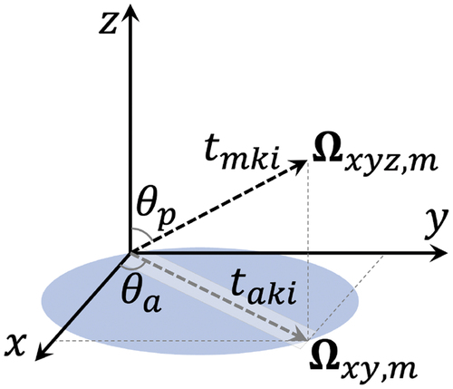
where ${\theta }_a$ = azimuthal angle and ${\theta }_p$ = polar angle. Note that the subscript $\mathit{a}$ of $t_{\mathit{aki}}$ denotes the variable is projected onto the $\mathit{x}-\mathit{y}$ plane. Also, note that the direction vector ${\mathbf{\Omega }}_{\mathit{xy},\mathit{m}}$ has information for the polar direction since it has $sin{\theta }_p$ in the $\mathit{x}$ and $\mathit{y}$ components. For the integration of an arbitrary variable $\mathit{f}$, the integral can be numerically evaluated from the tracking data generated by the ray-tracing procedure:

(3) $\left\{\begin{array}{c}{⟨\mathit{f}⟩}_i={\sum }_m{\omega }_m{⟨\mathit{f}⟩}_{\mathit{mi}}\\ {⟨\mathit{f}⟩}_{\mathit{mi}}=\frac{1}{V_i}{\sum }_k\mathit{\delta }{A}_{a}sin{\theta }_p{t}_{\mathit{mki}}{⟨\mathit{f}⟩}_{\mathit{mki}}\\ {⟨\mathit{f}⟩}_{\mathit{mki}}=\frac{1}{{\mathit{t}}_{\mathit{mki}}}{\int }_0^{{\mathit{t}}_{\mathit{mki}}}\mathit{f}(\mathit{t}{ }^{\mathrm{\prime }})\mathit{dt}{ }^{\mathrm{\prime }}\end{array}\right.,$(3)

where ${\omega }_m$ = quadrature weight for the discrete direction $\mathit{m}$ and is defined to be ${\sum }_m{\omega }_m=4\mathit{\pi }$; ${\theta }_p$ = polar angle between the segment and $\mathit{z}$-axis; $\mathit{\delta }{A}_a$ = width of the segment; $V_i$ = analytically calculated area of cell $\mathit{i}$.

As mentioned earlier, $t_{\mathit{mki}}$ is the renormalized MOC segment length defined as

(4) $t_{\mathit{mki}}={\xi }_{\mathit{ai}}{s}_{\mathit{mki}},$(4)

where $s_{\mathit{mki}}$ = MOC geometric segment length, which is numerically calculated by the ray tracing; ${\xi }_{\mathit{ai}}$ = renormalization factor to conserve the analytic volume of cell $\mathit{i}$. Note that the renormalization factor is determined in a direction-dependent way as follows:

(5) ${\xi }_{\mathit{ai}}=\frac{V_i}{{\sum }_k\mathit{\delta }{A}_a{s}_{\mathit{mki}}}.$(5)

We define $\mathbf{X}$ as the position variable in the global coordinate system. In the case of 2D geometry, $\mathbf{X}$ = ${\left[\mathit{X}\mathit{Y}\right]}^T$. Then, the local coordinates $\mathbf{x}$ (i.e., position relative to the centroid of a cell) are defined as

(6) $\mathbf{x}={\left[\mathit{x}\mathit{y}\right]}^T=\mathbf{X}-{\mathbf{X}}_{ai}^c,$(6)

where ${\mathbf{X}}_{ai}^c$ = numerical centroid of cell $\mathit{i}$ and is defined as ${\left[X_{ai}^c{Y}_{ai}^c\right]}^{\mathit{T}}$. The numerical centroid is calculated in a direction-dependent way by

(7) ${\mathbf{X}}_{ai}^c={⟨\mathbf{X}⟩}_{\mathit{mi}}.$(7)

The spatial coordinate $\mathbf{X}$ is related to $\mathit{t}$ by

(8) $\mathbf{X}={\mathbf{X}}_{aki}^{\mathrm{i}\mathrm{n}}+{\mathbf{\Omega }}_{\mathit{xy},\mathit{m}}\mathit{t}/{\xi }_{\mathit{ai}},$(8)

where ${\mathbf{X}}_{aki}^{\mathrm{i}\mathrm{n}}$ = starting location of the segment and is defined as ${\left[X_{aki}^{\mathrm{i}\mathrm{n}}{Y}_{aki}^{\mathrm{i}\mathrm{n}}\right]}^{\mathit{T}};$ $\mathit{t}$ = position along the length of the MOC segment with the range $0\le \mathit{t}\le t_{\mathit{mki}}$.

The moment-based LSA assumes that the shape of the source is spatially linear within each cell $\mathit{i}$. With the LIFA source, the source at position $\mathbf{x}$ in the direction $\mathit{m}$ can be expressed as

(9) $q_{mi}^g(\mathbf{x})={\bar{q}}_{\mathit{mi}}^{\mathit{g}}+\mathbf{x}\cdot {\hat{\mathbf{q}}}_{\mathit{i}}^{\mathit{g}},$(9)

where ${\bar{q}}_{\mathit{mi}}^{\mathit{g}}$ = flat portion of the source; ${\hat{\mathbf{q}}}_{\mathit{i}}^{\mathit{g}}$ = LS coefficient vector containing $\mathit{x}$ and $\mathit{y}$ components such that ${\hat{\mathbf{q}}}_{\mathit{i}}^{\mathit{g}}={\left[{\hat{q}}_{\mathit{x},\mathit{i}}^{\mathit{g}}{\hat{q}}_{\mathit{y},\mathit{i}}^{\mathit{g}}\right]}^{\mathit{T}}$. The flat portion of the source is expressed as

(10) ${\bar{q}}_{\mathit{mi}}^{\mathit{g}}=\frac{1}{4\mathit{\pi }}\left[\sum _{\mathit{l}=0}^L\sum _{\mathit{r}=-\mathit{l}}^l{R}_{lm}^r\sum _{\mathit{g}{\mathit{ }}^{\mathrm{\prime }}}{\mathrm{\Sigma }}_{\mathit{s},\mathit{li}}^{\mathit{g}{\mathit{ }}^{\mathrm{\prime }}\to \mathit{g}}{\bar{\varphi }}_{\mathit{li}}^{\mathit{rg}{ }^{\mathrm{\prime }}}+\frac{{\chi }_i^g}{k_{\mathrm{eff}}}\sum _{\mathit{g}{\mathit{ }}^{\mathrm{\prime }}}\mathit{\nu }{\mathrm{\Sigma }}_{\mathit{f},\mathit{i}}^{\mathit{g}{\mathit{ }}^{\mathrm{\prime }}}{\bar{\varphi }}_{\mathit{i}}^{\mathit{g}{ }^{\mathrm{\prime }}}\right],$(10)

where ${\mathrm{\Sigma }}_{\mathit{s},\mathit{li}}^{\mathit{g}{\mathit{ }}^{\mathrm{\prime }}\to \mathit{g}}$ = $\mathit{l}$’th order scattering matrix from group $\mathit{g}{ }^{\mathrm{\prime }}$ to $\mathit{g}$; $R_{lm}^r$ = real spherical harmonic in the direction ${\mathbf{\Omega }}_{\mathit{xyz},\mathit{m}}$^[26]; ${\bar{\varphi }}_{\mathit{li}}^{\mathit{rg}}$ = spatially flat angular flux moment and is defined as

(11) ${\bar{\varphi }}_{\mathit{li}}^{\mathit{rg}}={⟨R_{lm}^r{\psi }_{mki}^g(\mathit{t})⟩}_{\mathit{i}},$(11)

${\bar{\varphi }}_{\mathit{i}}^{\mathit{g}}$ = zeroth-order flux moment for brevity (${\bar{\varphi }}_{\mathit{i}}^{\mathit{g}}={\bar{\varphi }}_{0\mathit{i}}^{0\mathit{g}}$). The LS coefficients have only an isotropic component expressed as

(12) ${\hat{\mathbf{q}}}_{\mathit{i}}^{\mathit{g}}=\frac{1}{4\mathit{\pi }}\left[\sum _{\mathit{g}{\mathit{ }}^{\mathrm{\prime }}}{\mathrm{\Sigma }}_{\mathit{s},\mathit{i}}^{\mathit{g}{\mathit{ }}^{\mathrm{\prime }}\to \mathit{g}}{\widehat{\text{phii}}}_{\mathit{i}}^{\mathit{g}{ }^{\mathrm{\prime }}}+\frac{{\chi }_i^g}{k_{\mathrm{eff}}}\sum _{\mathit{g}{\mathit{ }}^{\mathrm{\prime }}}\mathit{\nu }{\mathrm{\Sigma }}_{\mathit{f},\mathit{i}}^{\mathit{g}{\mathit{ }}^{\mathrm{\prime }}}{\widehat{\text{phii}}}_{\mathit{i}}^{\mathit{g}{ }^{\mathrm{\prime }}}\right],$(12)

where ${\mathrm{\Sigma }}_{\mathit{s},\mathit{i}}^{\mathit{g}{\mathit{ }}^{\mathrm{\prime }}\to \mathit{g}}={\mathrm{\Sigma }}_{\mathit{s},0\mathit{i}}^{\mathit{g}{\mathit{ }}^{\mathrm{\prime }}\to \mathit{g}}$; ${\widehat{\text{phii}}}_{\mathit{i}}^{\mathit{g}}$ = linear flux moment coefficient vector containing $\mathit{x}$ and $\mathit{y}$ components such that ${\widehat{\text{phii}}}_{\mathit{i}}^{\mathit{g}}={\left[{\hat{\varphi }}_{\mathit{x},\mathit{i}}^{\mathit{g}}{\hat{\varphi }}_{\mathit{y},\mathit{i}}^{\mathit{g}}\right]}^{\mathit{T}}$. With this coefficient, the angular moments of the flux at position $\mathbf{x}$ are written as

(13) ${\varphi }_{li}^{rg}(\mathbf{x})={\bar{\varphi }}_{\mathit{li}}^{\mathit{rg}}+\mathbf{x}\cdot {\widehat{\text{phii}}}_{\mathit{i}}^{\mathit{g}}{\delta }_{0\mathit{l}},$(13)

where ${\delta }_{0\mathit{l}}$ = Kronecker delta. To determine the spatial expansion coefficients, Eq. (13)(13) ${\varphi }_{li}^{rg}(\mathbf{x})={\bar{\varphi }}_{\mathit{li}}^{\mathit{rg}}+\mathbf{x}\cdot {\widehat{\text{phii}}}_{\mathit{i}}^{\mathit{g}}{\delta }_{0\mathit{l}},$(13) is operated on by ${⟨\mathbf{x}(\cdot )⟩}_i$ for $\mathit{l}=0$. Recognizing that $\frac{1}{4\mathit{\pi }}{⟨\mathbf{x}{\varphi }_i^g(\mathbf{x})⟩}_{\mathit{i}}={⟨\mathbf{x}{\psi }_{mki}^g(\mathit{t})⟩}_{\mathit{i}}$, a system of equations is found:

(14) ${\mathbf{M}}_i{\widehat{\text{phii}}}_{\mathit{i}}^{\mathit{g}}={⟨\mathbf{x}{\psi }_{mki}^g(\mathit{t})⟩}_{\mathit{i}},$(14)

where

(15) $\begin{array}{rl}& {\mathbf{M}}_i=\frac{1}{4\mathit{\pi }}{⟨\mathbf{x}{\mathbf{x}}^T⟩}_{\mathit{i}}=\frac{1}{4\pi V_i}\sum _m{\omega }_m\sum _k\mathit{\delta }{A}_{a}sin{\theta }_p{t}_{\mathit{mki}}\\ & {⟨\left({\mathbf{x}}_{aki}^{\mathrm{i}\mathrm{n}}+{\mathbf{\Omega }}_{\mathit{xy},\mathit{m}}\mathit{t}/{\xi }_{\mathit{ai}}\right){\left({\mathbf{x}}_{aki}^{\mathrm{i}\mathrm{n}}+{\mathbf{\Omega }}_{\mathit{xy},\mathit{m}}\mathit{t}/{\xi }_{\mathit{ai}}\right)}^{\mathit{T}}⟩}_{\mathit{mki}}\\ & =\frac{1}{4\pi V_i}\sum _m{\omega }_m\sum _k\mathit{\delta }{A}_{a}sin{\theta }_p{t}_{\mathit{mki}}\\ & \left[{\mathbf{x}}_{aki}^c{\left({\mathbf{x}}_{aki}^c\right)}^{\mathit{T}}+\frac{{{\mathit{t}}_{\mathit{mki}}}^2}{12{{\mathit{\xi }}_{\mathit{ai}}}^2}{\mathbf{\Omega }}_{\mathit{xy},\mathit{m}}{{\mathbf{\Omega }}_{\mathit{xy},\mathit{m}}}^{\mathit{T}}\right],& (15)\end{array}$(15)

(16) $\mathbf{x}={\mathbf{x}}_{aki}^{\mathrm{i}\mathrm{n}}+{\mathbf{\Omega }}_{\mathit{xy},\mathit{m}}\mathit{t}/{\xi }_{\mathit{ai}},$(16)

with ${\mathbf{x}}_{aki}^{\mathrm{i}\mathrm{n}}$ as the starting point of the segment in the local coordinate. This is defined as ${\mathbf{x}}_{aki}^{\mathrm{i}\mathrm{n}}={\mathbf{X}}_{aki}^{\mathrm{i}\mathrm{n}}-{\mathbf{X}}_{ai}^c$. The value ${\mathbf{x}}_{aki}^c$ is the segment midpoint coordinates in the local coordinate system, and the relation to ${\mathbf{x}}_{aki}^{\mathrm{i}\mathrm{n}}$ is

(17) ${\mathbf{x}}_{aki}^c={\mathbf{x}}_{aki}^{\mathrm{i}\mathrm{n}}+{\mathbf{\Omega }}_{\mathit{xy},\mathit{m}}{t}_{\mathit{mki}}/\left(2{\xi }_{\mathit{ai}}\right).$(17)

Note that ${\mathbf{M}}_i$ in Eq. (15)(15) $\begin{array}{rl}& {\mathbf{M}}_i=\frac{1}{4\mathit{\pi }}{⟨\mathbf{x}{\mathbf{x}}^T⟩}_{\mathit{i}}=\frac{1}{4\pi V_i}\sum _m{\omega }_m\sum _k\mathit{\delta }{A}_{a}sin{\theta }_p{t}_{\mathit{mki}}\\ & {⟨\left({\mathbf{x}}_{aki}^{\mathrm{i}\mathrm{n}}+{\mathbf{\Omega }}_{\mathit{xy},\mathit{m}}\mathit{t}/{\xi }_{\mathit{ai}}\right){\left({\mathbf{x}}_{aki}^{\mathrm{i}\mathrm{n}}+{\mathbf{\Omega }}_{\mathit{xy},\mathit{m}}\mathit{t}/{\xi }_{\mathit{ai}}\right)}^{\mathit{T}}⟩}_{\mathit{mki}}\\ & =\frac{1}{4\pi V_i}\sum _m{\omega }_m\sum _k\mathit{\delta }{A}_{a}sin{\theta }_p{t}_{\mathit{mki}}\\ & \left[{\mathbf{x}}_{aki}^c{\left({\mathbf{x}}_{aki}^c\right)}^{\mathit{T}}+\frac{{{\mathit{t}}_{\mathit{mki}}}^2}{12{{\mathit{\xi }}_{\mathit{ai}}}^2}{\mathbf{\Omega }}_{\mathit{xy},\mathit{m}}{{\mathbf{\Omega }}_{\mathit{xy},\mathit{m}}}^{\mathit{T}}\right],& (15)\end{array}$(15) is the 2$\times$2 matrix for the 2D MOC and 2D/1D methods. The flux coefficients in ${\widehat{\text{phii}}}_{\mathit{i}}^{\mathit{g}}$ are solved by inverting Eq. (14)(14) ${\mathbf{M}}_i{\widehat{\text{phii}}}_{\mathit{i}}^{\mathit{g}}={⟨\mathbf{x}{\psi }_{mki}^g(\mathit{t})⟩}_{\mathit{i}},$(14) . The detailed expression for ${⟨\mathbf{x}{\psi }_{mki}^g⟩}_{\mathit{i}}$ in Eq. (14)(14) ${\mathbf{M}}_i{\widehat{\text{phii}}}_{\mathit{i}}^{\mathit{g}}={⟨\mathbf{x}{\psi }_{mki}^g(\mathit{t})⟩}_{\mathit{i}},$(14) is defined later.

With the assumed shape of the source in Eq. (9)(9) $q_{mi}^g(\mathbf{x})={\bar{q}}_{\mathit{mi}}^{\mathit{g}}+\mathbf{x}\cdot {\hat{\mathbf{q}}}_{\mathit{i}}^{\mathit{g}},$(9) , the LS along a MOC segment is

(18) $q_{mki}^g(\mathit{t})={\bar{q}}_{\mathit{mki}}^{\mathit{g}}+{\hat{q}}_{\mathit{mi}}^{\mathit{g}}\left(\mathit{t}-\frac{{\mathit{t}}_{\mathit{mki}}}{2}\right),$(18)

where

(19) ${\bar{q}}_{\mathit{mki}}^{\mathit{g}}={\bar{q}}_{\mathit{mi}}^{\mathit{g}}+{\mathbf{x}}_{aki}^c\cdot {\hat{\mathbf{q}}}_{\mathit{i}}^{\mathit{g}},$(19)

(20) ${\hat{q}}_{\mathit{mi}}^{\mathit{g}}={\mathbf{\Omega }}_{\mathit{xy},\mathit{m}}\cdot {\hat{\mathbf{q}}}_{\mathit{i}}^{\mathit{g}}/{\xi }_{\mathit{ai}}.$(20)

The LS coefficient ${\hat{\mathbf{q}}}_{\mathit{i}}^{\mathit{g}}$ is defined later. Using the expression for the source in Eq. (18)(18) $q_{mki}^g(\mathit{t})={\bar{q}}_{\mathit{mki}}^{\mathit{g}}+{\hat{q}}_{\mathit{mi}}^{\mathit{g}}\left(\mathit{t}-\frac{{\mathit{t}}_{\mathit{mki}}}{2}\right),$(18) , the characteristic transport equation becomes

(21) $\frac{d{\psi }_{mki}^g(\mathit{t})}{\mathit{dt}}+{\mathrm{\Sigma }}_{t,i}^g{\psi }_{mki}^g(\mathit{t})={\bar{q}}_{\mathit{mki}}^{\mathit{g}}+{\hat{q}}_{\mathit{mi}}^{\mathit{g}}\left(\mathit{t}-\frac{{\mathit{t}}_{\mathit{mki}}}{2}\right).$(21)

The solution of Eq. (21)(21) $\frac{d{\psi }_{mki}^g(\mathit{t})}{\mathit{dt}}+{\mathrm{\Sigma }}_{t,i}^g{\psi }_{mki}^g(\mathit{t})={\bar{q}}_{\mathit{mki}}^{\mathit{g}}+{\hat{q}}_{\mathit{mi}}^{\mathit{g}}\left(\mathit{t}-\frac{{\mathit{t}}_{\mathit{mki}}}{2}\right).$(21) is

(22) ${\psi }_{mki}^g(\mathit{t})={\psi }_{mki}^{g,\mathrm{i}\mathrm{n}}+\left(\frac{{\bar{q}}_{\mathit{mki}}^{\mathit{g}}}{{\mathrm{\Sigma }}_{t,i}^g}-{\psi }_{mki}^{g,\mathrm{i}\mathrm{n}}\right)F_1(\mathit{\tau })+\frac{{\hat{q}}_{\mathit{mi}}^{\mathit{g}}}{2{\mathrm{\Sigma }}_{t,i}^g}\frac{F_2(\mathit{\tau })}{{\mathrm{\Sigma }}_{t,i}^g},$(22)

where we have defined

(23) $F_1(\mathit{\tau })=1-e^{-\mathit{\tau }},$(23)

(24) $F_2(\mathit{\tau })=2\left[\mathit{\tau }-F_1(\mathit{\tau })\right]-{\tau }_{mki}^g{F}_1(\mathit{\tau }),$(24)

$\mathit{\tau }$ = optical thickness defined as ${\mathrm{\Sigma }}_{t,i}^g\mathit{t}$; ${\tau }_{mki}^g={\mathrm{\Sigma }}_{t,i}^g{t}_{\mathit{mki}}$; ${\psi }_{mki}^{g,\mathrm{i}\mathrm{n}}$ = incoming angular flux and is equivalent to ${\psi }_{mki}^g(0)$.

The track-averaged angular flux is determined by operating ${⟨\left(\cdot \right)⟩}_{\mathit{mki}}$ on Eq. (21)(21) $\frac{d{\psi }_{mki}^g(\mathit{t})}{\mathit{dt}}+{\mathrm{\Sigma }}_{t,i}^g{\psi }_{mki}^g(\mathit{t})={\bar{q}}_{\mathit{mki}}^{\mathit{g}}+{\hat{q}}_{\mathit{mi}}^{\mathit{g}}\left(\mathit{t}-\frac{{\mathit{t}}_{\mathit{mki}}}{2}\right).$(21) , yielding

(25) $\begin{array}{rl}& {\bar{\psi }}_{\mathit{mki}}^{\mathit{g}}={⟨{\psi }_{mki}^g(\mathit{t})⟩}_{\mathit{mki}}\\ & =\frac{{\bar{q}}_{\mathit{mki}}^{\mathit{g}}}{{\mathrm{\Sigma }}_{t,i}^g}+\frac{\mathrm{\Delta }{\psi }_{mki}^g}{{\tau }_{mki}^g},& (25)\end{array}$(25)

where $\mathrm{\Delta }{\psi }_{mki}^g$ = difference between the incoming angular flux and outgoing angular flux, namely, $\mathrm{\Delta }{\psi }_{mki}^g={\psi }_{mki}^{g,\mathrm{i}\mathrm{n}}-{\psi }_{mki}^{g,\mathrm{o}\mathrm{u}\mathrm{t}}$; ${\psi }_{mki}^{g,\mathrm{o}\mathrm{u}\mathrm{t}}$ = outgoing angular flux and is equivalent to ${\psi }_{mki}^g(t_{\mathit{mki}})$. The first spatial moment of the angular flux is found by operating ${⟨\mathit{t}\left(\cdot \right)⟩}_{\mathit{mki}}$ on Eq. (21)(21) $\frac{d{\psi }_{mki}^g(\mathit{t})}{\mathit{dt}}+{\mathrm{\Sigma }}_{t,i}^g{\psi }_{mki}^g(\mathit{t})={\bar{q}}_{\mathit{mki}}^{\mathit{g}}+{\hat{q}}_{\mathit{mi}}^{\mathit{g}}\left(\mathit{t}-\frac{{\mathit{t}}_{\mathit{mki}}}{2}\right).$(21) , yielding

(26) $\begin{array}{rl}{\hat{\psi }}_{\mathit{mki}}^{\mathit{g}}& ={⟨t{\psi }_{mki}^g(\mathit{t})⟩}_{\mathit{mki}}\\ \mathit{\hspace{0.17em}}& =\frac{{\bar{\psi }}_{\mathit{mki}}^{\mathit{g}}-{\psi }_{mki}^{g,\mathrm{o}\mathrm{u}\mathrm{t}}}{{\mathrm{\Sigma }}_{t,i}^g}+\frac{{\mathit{t}}_{\mathit{mki}}}{2}\left[\frac{{\bar{q}}_{\mathit{mki}}^{\mathit{g}}}{{\mathrm{\Sigma }}_{t,i}^g}+\frac{{\hat{q}}_{\mathit{mi}}^{\mathit{g}}}{{\mathrm{\Sigma }}_{t,i}^g}\frac{{\mathit{t}}_{\mathit{mki}}}{6}\right].\end{array}$(26)

Note that no new exponential function has been introduced. The value ${\hat{\psi }}_{\mathit{mki}}^{\mathit{g}}$ is used to derive ${⟨\mathbf{x}{\psi }_{mki}^g(\mathit{t})⟩}_{\mathit{i}}$ later. Next, we define the new quantity

(27) $\mathit{\psi }{{\mathit{ }}^{\mathrm{\prime }}}_{\mathit{mki}}^{\mathit{g}}=\mathrm{\Delta }{\psi }_{mki}^g/{\tau }_{mki}^g,$(27)

where $\mathit{\psi }{{\mathit{ }}^{\mathrm{\prime }}}_{\mathit{mki}}^{\mathit{g}}$ will be used in the calculations of region average flux and flux moments. The value $\mathit{\psi }{{\mathit{ }}^{\mathrm{\prime }}}_{\mathit{mki}}^{\mathit{g}}$ is computed during the transmission calculation with the following formulation:

(28) $\mathit{\psi }{{\mathit{ }}^{\mathrm{\prime }}}_{\mathit{mki}}^{\mathit{g}}=\left({\psi }_{mki}^{g,in}-\frac{{\bar{q}}_{\mathit{mki}}^{\mathit{g}}}{{\mathrm{\Sigma }}_{t,i}^g}\right)E_1({\tau }_{mki}^g)-\frac{{\mathit{t}}_{\mathit{mki}}}{2}\frac{{\hat{q}}_{\mathit{mi}}^{\mathit{g}}}{{\mathrm{\Sigma }}_{t,i}^g}{E}_2({\tau }_{mki}^g),$(28)

where

(29) $E_1({\tau }_{mki}^g)=\frac{F_1({\tau }_{mki}^g)}{{\tau }_{mki}^g}=\frac{1-e^{-{\tau }_{mki}^g}}{{\tau }_{mki}^g},$(29)

(30) $E_2({\tau }_{mki}^g)=2E_3({\tau }_{mki}^g)-E_1({\tau }_{mki}^g),$(30)

and

(31) $E_3({\tau }_{mki}^g)=\frac{1-E_1({\tau }_{mki}^g)}{{\tau }_{mki}^g}.$(31)

Here, $E_3(\mathit{\tau })$ is defined as an intermediate function that has smaller derivative terms than $F_1(\mathit{\tau })$, meaning higher accuracy with fewer interpolation intervals. Only the $E_3(\mathit{\tau })$ function needs to be tabulated. Then, it can be used to compute the other two exponential functions, $E_1(\mathit{\tau })$ and $E_2(\mathit{\tau })$. More detailed information about usage of $E_3(\mathit{\tau })$ is described in Sec. II.A.1.

In the actual calculation, it is beneficial to compute $\mathit{\psi }{{\mathit{ }}^{\mathrm{\prime }}}_{\mathit{mki}}^{\mathit{g}}$ directly for numerical stability rather than calculating $\mathrm{\Delta }{\psi }_{mki}^g$ and performing division. Given this formulation, the outgoing angular flux can be evaluated as

(32) ${\psi }_{mki}^{g,\mathrm{o}\mathrm{u}\mathrm{t}}={\psi }_{mki}^{g,\mathrm{i}\mathrm{n}}-{\tau }_{mki}^g\mathit{\psi }{{\mathit{ }}^{\mathrm{\prime }}}_{\mathit{mki}}^{\mathit{g}}.$(32)

Using Eqs. (16)(16) $\mathbf{x}={\mathbf{x}}_{aki}^{\mathrm{i}\mathrm{n}}+{\mathbf{\Omega }}_{\mathit{xy},\mathit{m}}\mathit{t}/{\xi }_{\mathit{ai}},$(16) and (26)(26) $\begin{array}{rl}{\hat{\psi }}_{\mathit{mki}}^{\mathit{g}}& ={⟨t{\psi }_{mki}^g(\mathit{t})⟩}_{\mathit{mki}}\\ \mathit{\hspace{0.17em}}& =\frac{{\bar{\psi }}_{\mathit{mki}}^{\mathit{g}}-{\psi }_{mki}^{g,\mathrm{o}\mathrm{u}\mathrm{t}}}{{\mathrm{\Sigma }}_{t,i}^g}+\frac{{\mathit{t}}_{\mathit{mki}}}{2}\left[\frac{{\bar{q}}_{\mathit{mki}}^{\mathit{g}}}{{\mathrm{\Sigma }}_{t,i}^g}+\frac{{\hat{q}}_{\mathit{mi}}^{\mathit{g}}}{{\mathrm{\Sigma }}_{t,i}^g}\frac{{\mathit{t}}_{\mathit{mki}}}{6}\right].\end{array}$(26) , the flux moment is then written as

(33) $\begin{array}{rl}& {⟨\mathbf{x}{\psi }_{mki}^g(\mathit{t})⟩}_{\mathit{i}}=\frac{4\mathit{\pi }{\mathbf{M}}_i{\hat{\mathbf{q}}}_{\mathit{i}}^{\mathit{g}}}{{\mathrm{\Sigma }}_{t,i}^g}+\frac{1}{{\mathrm{\Sigma }}_{t,i}^g{V}_i}\sum _m{\omega }_m\sum _k\mathit{\delta }{A}_{a}sin{\theta }_p\\ & [{\mathbf{x}}_{aki}^{\mathrm{i}\mathrm{n}}{\tau }_{mki}^g\mathit{\psi }{{\mathit{ }}^{\mathrm{\prime }}}_{\mathit{mki}}^{\mathit{g}}+{\mathbf{\Omega }}_{\mathit{xy},\mathit{m}}\frac{{\mathit{t}}_{\mathit{mki}}}{{\xi }_{\mathit{ai}}}\\ & \left.\left(\frac{{\bar{q}}_{\mathit{mi}}^{\mathit{g}}}{{\mathrm{\Sigma }}_{t,i}^g}+\mathit{\psi }{{\mathit{ }}^{\mathrm{\prime }}}_{\mathit{mki}}^{\mathit{g}}-{\psi }_{mki}^{g,\mathrm{o}\mathrm{u}\mathrm{t}}\right)\right].& (33)\end{array}$(33)

The scalar flux in Eq. (11)(11) ${\bar{\varphi }}_{\mathit{li}}^{\mathit{rg}}={⟨R_{lm}^r{\psi }_{mki}^g(\mathit{t})⟩}_{\mathit{i}},$(11) is now expanded to

(34) $\begin{array}{rl}& {\bar{\varphi }}_{\mathit{li}}^{\mathit{rg}}=\frac{1}{{\mathrm{\Sigma }}_{t,i}^g}\sum _m{\omega }_m{R}_{lm}^r{\bar{q}}_{\mathit{mi}}^{\mathit{g}}+\frac{1}{V_i{\mathrm{\Sigma }}_{t,i}^g}\sum _m{\omega }_m{R}_{lm}^r\\ & \sum _k\mathit{\delta }{A}_{a}sin{\theta }_p{\tau }_{mki}^g\mathit{\psi }{{\mathit{ }}^{\mathrm{\prime }}}_{\mathit{mki}}^{\mathit{g}}.& (34)\end{array}$(34)

If P₀ or Transport-Corrected P₀ (TCP₀) isotropic scattering approximations are used, then several equations can be simplified.

The region average source ${\bar{q}}_{\mathit{mi}}^{\mathit{g}}$ in Eq. (10)(10) ${\bar{q}}_{\mathit{mi}}^{\mathit{g}}=\frac{1}{4\mathit{\pi }}\left[\sum _{\mathit{l}=0}^L\sum _{\mathit{r}=-\mathit{l}}^l{R}_{lm}^r\sum _{\mathit{g}{\mathit{ }}^{\mathrm{\prime }}}{\mathrm{\Sigma }}_{\mathit{s},\mathit{li}}^{\mathit{g}{\mathit{ }}^{\mathrm{\prime }}\to \mathit{g}}{\bar{\varphi }}_{\mathit{li}}^{\mathit{rg}{ }^{\mathrm{\prime }}}+\frac{{\chi }_i^g}{k_{\mathrm{eff}}}\sum _{\mathit{g}{\mathit{ }}^{\mathrm{\prime }}}\mathit{\nu }{\mathrm{\Sigma }}_{\mathit{f},\mathit{i}}^{\mathit{g}{\mathit{ }}^{\mathrm{\prime }}}{\bar{\varphi }}_{\mathit{i}}^{\mathit{g}{ }^{\mathrm{\prime }}}\right],$(10) does not have angle dependency in the case of P₀, and it is rewritten as follows:

(35) ${\bar{q}}_{\mathit{i}}^{\mathit{g}}=\frac{1}{4\mathit{\pi }}\left[\sum _{\mathit{g}{\mathit{ }}^{\mathrm{\prime }}}{\mathrm{\Sigma }}_{\mathit{s},\mathit{i}}^{\mathit{g}{\mathit{ }}^{\mathrm{\prime }}\to \mathit{g}}{\bar{\varphi }}_{\mathit{i}}^{\mathit{g}{ }^{\mathrm{\prime }}}+\frac{{\chi }_i^g}{k_{\mathit{eff}}}\sum _{\mathit{g}{\mathit{ }}^{\mathrm{\prime }}}\mathit{\nu }{\mathrm{\Sigma }}_{\mathit{f},\mathit{i}}^{\mathit{g}{\mathit{ }}^{\mathrm{\prime }}}{\bar{\varphi }}_{\mathit{i}}^{\mathit{g}{ }^{\mathrm{\prime }}}\right],$(35)

where ${\bar{q}}_{\mathit{i}}^{\mathit{g}}$ is the same as ${\bar{q}}_{\mathit{mi}}^{\mathit{g}}$ defined in Eq. (10)(10) ${\bar{q}}_{\mathit{mi}}^{\mathit{g}}=\frac{1}{4\mathit{\pi }}\left[\sum _{\mathit{l}=0}^L\sum _{\mathit{r}=-\mathit{l}}^l{R}_{lm}^r\sum _{\mathit{g}{\mathit{ }}^{\mathrm{\prime }}}{\mathrm{\Sigma }}_{\mathit{s},\mathit{li}}^{\mathit{g}{\mathit{ }}^{\mathrm{\prime }}\to \mathit{g}}{\bar{\varphi }}_{\mathit{li}}^{\mathit{rg}{ }^{\mathrm{\prime }}}+\frac{{\chi }_i^g}{k_{\mathrm{eff}}}\sum _{\mathit{g}{\mathit{ }}^{\mathrm{\prime }}}\mathit{\nu }{\mathrm{\Sigma }}_{\mathit{f},\mathit{i}}^{\mathit{g}{\mathit{ }}^{\mathrm{\prime }}}{\bar{\varphi }}_{\mathit{i}}^{\mathit{g}{ }^{\mathrm{\prime }}}\right],$(10) but it is a special case for $\mathit{L}=0$. Since ${\bar{q}}_{\mathit{i}}^{\mathit{g}}$ does not have angle dependency, the segment average source ${\bar{q}}_{\mathit{mki}}^{\mathit{g}}$ is also simplified to ${\bar{q}}_{\mathit{aki}}^{\mathit{g}}$ to have only azimuthal angle dependency instead of both azimuthal and polar angles:

(36) ${\bar{q}}_{\mathit{aki}}^{\mathit{g}}={\bar{q}}_{\mathit{i}}^{\mathit{g}}+{\mathbf{x}}_{aki}^{\mathrm{c}}\cdot {\hat{\mathbf{q}}}_{\mathit{i}}^{\mathit{g}}.$(36)

The value ${\bar{q}}_{\mathit{mki}}^{\mathit{g}}$ in Eq. (28)(28) $\mathit{\psi }{{\mathit{ }}^{\mathrm{\prime }}}_{\mathit{mki}}^{\mathit{g}}=\left({\psi }_{mki}^{g,in}-\frac{{\bar{q}}_{\mathit{mki}}^{\mathit{g}}}{{\mathrm{\Sigma }}_{t,i}^g}\right)E_1({\tau }_{mki}^g)-\frac{{\mathit{t}}_{\mathit{mki}}}{2}\frac{{\hat{q}}_{\mathit{mi}}^{\mathit{g}}}{{\mathrm{\Sigma }}_{t,i}^g}{E}_2({\tau }_{mki}^g),$(28) is replaced by this ${\bar{q}}_{\mathit{aki}}^{\mathit{g}}$ for the calculation of $\mathit{\psi }{{\mathit{ }}^{\mathrm{\prime }}}_{\mathit{mki}}^{\mathit{g}}$. ${⟨\mathbf{x}{\psi }_{mki}^g(\mathit{t})⟩}_{\mathit{i}}$ is simplified as

(37) $\begin{array}{rl}& {⟨\mathbf{x}{\psi }_{mki}^g(\mathit{t})⟩}_{\mathit{i}}=\frac{4\mathit{\pi }{\mathbf{M}}_i{\hat{\mathbf{q}}}_{\mathit{i}}^{\mathit{g}}}{{\mathrm{\Sigma }}_{t,i}^g}+\frac{1}{{\mathrm{\Sigma }}_{t,i}^g{V}_i}\sum _m{\omega }_m\\ & \sum _k\mathit{\delta }{A}_{a}sin{\theta }_p[{\mathbf{x}}_{aki}^{\mathrm{i}\mathrm{n}}\mathrm{\Delta }{\psi }_{mki}^g\\ & \left.+{\mathbf{\Omega }}_{\mathit{xy},\mathit{m}}\frac{{\mathit{t}}_{\mathit{mki}}}{{\xi }_{\mathit{ai}}}\left(\mathit{\psi }{{\mathit{ }}^{\mathrm{\prime }}}_{\mathit{mki}}^{\mathit{g}}-{\psi }_{mki}^{g,\mathrm{o}\mathrm{u}\mathrm{t}}\right)\right].& (37)\end{array}$(37)

The scalar flux is also simplified to

(38) $\begin{array}{rl}& {\bar{\varphi }}_{\mathit{i}}^{\mathit{g}}=\frac{1}{{\mathrm{\Sigma }}_{t,i}^g}\sum _m{\omega }_m{\bar{q}}_{\mathit{i}}^{\mathit{g}}+\frac{1}{V_i{\mathrm{\Sigma }}_{t,i}^g}\sum _m{\omega }_m\\ & \sum _k\mathit{\delta }{A}_{a}sin{\theta }_p{\tau }_{mki}^g\mathit{\psi }{{\mathit{ }}^{\mathrm{\prime }}}_{\mathit{mki}}^{\mathit{g}}.& (38)\end{array}$(38)

Equations (10)(10) ${\bar{q}}_{\mathit{mi}}^{\mathit{g}}=\frac{1}{4\mathit{\pi }}\left[\sum _{\mathit{l}=0}^L\sum _{\mathit{r}=-\mathit{l}}^l{R}_{lm}^r\sum _{\mathit{g}{\mathit{ }}^{\mathrm{\prime }}}{\mathrm{\Sigma }}_{\mathit{s},\mathit{li}}^{\mathit{g}{\mathit{ }}^{\mathrm{\prime }}\to \mathit{g}}{\bar{\varphi }}_{\mathit{li}}^{\mathit{rg}{ }^{\mathrm{\prime }}}+\frac{{\chi }_i^g}{k_{\mathrm{eff}}}\sum _{\mathit{g}{\mathit{ }}^{\mathrm{\prime }}}\mathit{\nu }{\mathrm{\Sigma }}_{\mathit{f},\mathit{i}}^{\mathit{g}{\mathit{ }}^{\mathrm{\prime }}}{\bar{\varphi }}_{\mathit{i}}^{\mathit{g}{ }^{\mathrm{\prime }}}\right],$(10) , (12)(12) ${\hat{\mathbf{q}}}_{\mathit{i}}^{\mathit{g}}=\frac{1}{4\mathit{\pi }}\left[\sum _{\mathit{g}{\mathit{ }}^{\mathrm{\prime }}}{\mathrm{\Sigma }}_{\mathit{s},\mathit{i}}^{\mathit{g}{\mathit{ }}^{\mathrm{\prime }}\to \mathit{g}}{\widehat{\text{phii}}}_{\mathit{i}}^{\mathit{g}{ }^{\mathrm{\prime }}}+\frac{{\chi }_i^g}{k_{\mathrm{eff}}}\sum _{\mathit{g}{\mathit{ }}^{\mathrm{\prime }}}\mathit{\nu }{\mathrm{\Sigma }}_{\mathit{f},\mathit{i}}^{\mathit{g}{\mathit{ }}^{\mathrm{\prime }}}{\widehat{\text{phii}}}_{\mathit{i}}^{\mathit{g}{ }^{\mathrm{\prime }}}\right],$(12) , (14)(14) ${\mathbf{M}}_i{\widehat{\text{phii}}}_{\mathit{i}}^{\mathit{g}}={⟨\mathbf{x}{\psi }_{mki}^g(\mathit{t})⟩}_{\mathit{i}},$(14) , (19)(19) ${\bar{q}}_{\mathit{mki}}^{\mathit{g}}={\bar{q}}_{\mathit{mi}}^{\mathit{g}}+{\mathbf{x}}_{aki}^c\cdot {\hat{\mathbf{q}}}_{\mathit{i}}^{\mathit{g}},$(19) , (20)(20) ${\hat{q}}_{\mathit{mi}}^{\mathit{g}}={\mathbf{\Omega }}_{\mathit{xy},\mathit{m}}\cdot {\hat{\mathbf{q}}}_{\mathit{i}}^{\mathit{g}}/{\xi }_{\mathit{ai}}.$(20) , (28)(28) $\mathit{\psi }{{\mathit{ }}^{\mathrm{\prime }}}_{\mathit{mki}}^{\mathit{g}}=\left({\psi }_{mki}^{g,in}-\frac{{\bar{q}}_{\mathit{mki}}^{\mathit{g}}}{{\mathrm{\Sigma }}_{t,i}^g}\right)E_1({\tau }_{mki}^g)-\frac{{\mathit{t}}_{\mathit{mki}}}{2}\frac{{\hat{q}}_{\mathit{mi}}^{\mathit{g}}}{{\mathrm{\Sigma }}_{t,i}^g}{E}_2({\tau }_{mki}^g),$(28) , (32)(32) ${\psi }_{mki}^{g,\mathrm{o}\mathrm{u}\mathrm{t}}={\psi }_{mki}^{g,\mathrm{i}\mathrm{n}}-{\tau }_{mki}^g\mathit{\psi }{{\mathit{ }}^{\mathrm{\prime }}}_{\mathit{mki}}^{\mathit{g}}.$(32) through (35)(35) ${\bar{q}}_{\mathit{i}}^{\mathit{g}}=\frac{1}{4\mathit{\pi }}\left[\sum _{\mathit{g}{\mathit{ }}^{\mathrm{\prime }}}{\mathrm{\Sigma }}_{\mathit{s},\mathit{i}}^{\mathit{g}{\mathit{ }}^{\mathrm{\prime }}\to \mathit{g}}{\bar{\varphi }}_{\mathit{i}}^{\mathit{g}{ }^{\mathrm{\prime }}}+\frac{{\chi }_i^g}{k_{\mathit{eff}}}\sum _{\mathit{g}{\mathit{ }}^{\mathrm{\prime }}}\mathit{\nu }{\mathrm{\Sigma }}_{\mathit{f},\mathit{i}}^{\mathit{g}{\mathit{ }}^{\mathrm{\prime }}}{\bar{\varphi }}_{\mathit{i}}^{\mathit{g}{ }^{\mathrm{\prime }}}\right],$(35) , (37)(37) $\begin{array}{rl}& {⟨\mathbf{x}{\psi }_{mki}^g(\mathit{t})⟩}_{\mathit{i}}=\frac{4\mathit{\pi }{\mathbf{M}}_i{\hat{\mathbf{q}}}_{\mathit{i}}^{\mathit{g}}}{{\mathrm{\Sigma }}_{t,i}^g}+\frac{1}{{\mathrm{\Sigma }}_{t,i}^g{V}_i}\sum _m{\omega }_m\\ & \sum _k\mathit{\delta }{A}_{a}sin{\theta }_p[{\mathbf{x}}_{aki}^{\mathrm{i}\mathrm{n}}\mathrm{\Delta }{\psi }_{mki}^g\\ & \left.+{\mathbf{\Omega }}_{\mathit{xy},\mathit{m}}\frac{{\mathit{t}}_{\mathit{mki}}}{{\xi }_{\mathit{ai}}}\left(\mathit{\psi }{{\mathit{ }}^{\mathrm{\prime }}}_{\mathit{mki}}^{\mathit{g}}-{\psi }_{mki}^{g,\mathrm{o}\mathrm{u}\mathrm{t}}\right)\right].& (37)\end{array}$(37) , and (38)(38) $\begin{array}{rl}& {\bar{\varphi }}_{\mathit{i}}^{\mathit{g}}=\frac{1}{{\mathrm{\Sigma }}_{t,i}^g}\sum _m{\omega }_m{\bar{q}}_{\mathit{i}}^{\mathit{g}}+\frac{1}{V_i{\mathrm{\Sigma }}_{t,i}^g}\sum _m{\omega }_m\\ & \sum _k\mathit{\delta }{A}_{a}sin{\theta }_p{\tau }_{mki}^g\mathit{\psi }{{\mathit{ }}^{\mathrm{\prime }}}_{\mathit{mki}}^{\mathit{g}}.& (38)\end{array}$(38) represent the final forms of the LS MOC equations used in MPACT. Sections II.A.1 and II.A.2 will present several subtle, but important, details for their implementation.

II.A.1. Exponential Table

In conventional flat source (FS) MOC calculations, the exponential function is normally tabulated and then linearly interpolated at run time.^[27,28] This is because the exponential calculation is one of the most computationally expensive floating point operations among the MOC calculation. In FSA, the $F_1(\mathit{\tau })$ function in Eq. (23)(23) $F_1(\mathit{\tau })=1-e^{-\mathit{\tau }},$(23) is tabulated. The tabulation of the exponential function requires special treatment around $\mathit{\tau }=0$ to prevent issues arising from limited significant digits. This is normally handled via Taylor expansion around $\mathit{\tau }=0$.

A similar approach is used for the LSA in this work. As described in the Sec. II.A, the $E_3(\mathit{\tau })$ function in Eq. (31)(31) $E_3({\tau }_{mki}^g)=\frac{1-E_1({\tau }_{mki}^g)}{{\tau }_{mki}^g}.$(31) is only tabulated as a function of $\mathit{\tau }$ and then used through linear interpolation to calculate $E_1(\mathit{\tau }),$ $E_2(\mathit{\tau }),$ and then the flux. In traditional implementations for the exponential function tabulation,^[27,28] evenly spaced interpolation points within each interval are normally used. However, this does not minimize the error in the approximation. In this work, the Chebyshev points^[29] are used to minimize the error from the interpolation. Fitzgerald and Kochunas^[30] showed that an interpolation table using Chebyshev points reduces the interpolation error by half at no run-time cost compared to a table using evenly spaced points.

It is also worthwhile to mention why we tabulate $E_3(\mathit{\tau })$ instead of the $F_1(\mathit{\tau })$ or $F_2(\mathit{\tau })$ functions. In MPACT,^[2] the FS MOC solver uses a double-precision linear interpolation table of $F_1(\mathit{\tau })$ with maximum error on the order of ${10}^{-7}$. This accuracy was found to be sufficient for problems of interest. With the implementation of a LS MOC solver into MPACT, stability issues were observed in problems having spatial cells with low total cross sections, such as the fuel-clad gap in LWRs. These stability issues occurred only when the exponential functions were approximated. This seemed to indicate that more accurate interpolation was necessary.

In the original derivation of LSA,^[9] the outgoing angular flux is explicitly calculated by Eq. (22)(22) ${\psi }_{mki}^g(\mathit{t})={\psi }_{mki}^{g,\mathrm{i}\mathrm{n}}+\left(\frac{{\bar{q}}_{\mathit{mki}}^{\mathit{g}}}{{\mathrm{\Sigma }}_{t,i}^g}-{\psi }_{mki}^{g,\mathrm{i}\mathrm{n}}\right)F_1(\mathit{\tau })+\frac{{\hat{q}}_{\mathit{mi}}^{\mathit{g}}}{2{\mathrm{\Sigma }}_{t,i}^g}\frac{F_2(\mathit{\tau })}{{\mathrm{\Sigma }}_{t,i}^g},$(22) and then used in the subsequent calculation. In Eq. (22)(22) ${\psi }_{mki}^g(\mathit{t})={\psi }_{mki}^{g,\mathrm{i}\mathrm{n}}+\left(\frac{{\bar{q}}_{\mathit{mki}}^{\mathit{g}}}{{\mathrm{\Sigma }}_{t,i}^g}-{\psi }_{mki}^{g,\mathrm{i}\mathrm{n}}\right)F_1(\mathit{\tau })+\frac{{\hat{q}}_{\mathit{mi}}^{\mathit{g}}}{2{\mathrm{\Sigma }}_{t,i}^g}\frac{F_2(\mathit{\tau })}{{\mathrm{\Sigma }}_{t,i}^g},$(22) , the $F_2(\mathit{\tau })$ function appears with an inverse total cross-section term. This means that any error in $F_2(\mathit{\tau })$ will be magnified by the inverse of the total cross section. This issue may be resolved by tabulating $F_2(\mathit{\tau })/{\mathrm{\Sigma }}_{t,i}^g$. It is likely that the actual implementation of CASMO5 addressed this issue, but it is not described in the original paper^[9] and does not appear to be described in the open literature. We have found that tabulation of the $E_3(\mathit{\tau })$ function and use of the result to compute $E_1(\mathit{\tau })$ and $E_2(\mathit{\tau })$ are efficient and robust. This is why we reformulate the LSA derivation to compute $\mathit{\psi }{{\mathit{ }}^{\mathrm{\prime }}}_{\mathit{mki}}^{\mathit{g}}$ in Eq. (28)(28) $\mathit{\psi }{{\mathit{ }}^{\mathrm{\prime }}}_{\mathit{mki}}^{\mathit{g}}=\left({\psi }_{mki}^{g,in}-\frac{{\bar{q}}_{\mathit{mki}}^{\mathit{g}}}{{\mathrm{\Sigma }}_{t,i}^g}\right)E_1({\tau }_{mki}^g)-\frac{{\mathit{t}}_{\mathit{mki}}}{2}\frac{{\hat{q}}_{\mathit{mi}}^{\mathit{g}}}{{\mathrm{\Sigma }}_{t,i}^g}{E}_2({\tau }_{mki}^g),$(28) instead of computing $\mathrm{\Delta }{\psi }_{mki}^g$ or ${\psi }_{mki}^{g,\mathrm{o}\mathrm{u}\mathrm{t}}$ explicitly.

There is also a downside to using $E_3(\mathit{\tau })$. The value $E_3(\mathit{\tau })$ is tabulated between 0 and ${\tau }^{\max }$. The maximum value of $\mathit{\tau }$ (i.e., ${\tau }^{\max }$) in MPACT is 40, which may be sufficiently large for the 2D calculation. However, the $\mathit{\tau }$ value can exceed the maximum limit of the table in the case of 2D/1D calculation when the total cross section may become very large due to the TL splitting. 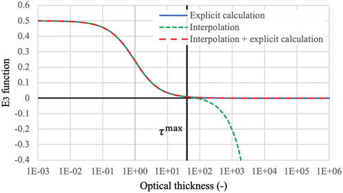When $\mathit{\tau }$ exceeds the range of the table, $E_3(\mathit{\tau })$ should not be extrapolated because it can result in a negative value as shown in Fig. 2.

Fig. 2. $E_3(\mathit{\tau })$ function calculation.

The $F_1(\mathit{\tau })$ function for FS MOC does not have this issue. In the double-precision calculation, $F_1(40)$ and $F_1(\mathrm{\infty })$ are both 1 to the same, sufficient precision. In the single precision, $\mathit{\tau }=20$ gives 1 beyond the necessary precision. Therefore, the extrapolation of $F_1(\mathit{\tau })$ over ${\tau }^{\max }$ also gives 1.

However, the $E_3(\mathit{\tau })$ function in this paper is not sufficiently close to 0 [i.e., the limit of $E_3(\mathrm{\infty })$] when $\mathit{\tau }$ is near ${\tau }^{\max }$ due to the scaling by the inverse of optical thickness in Eq. (31)(31) $E_3({\tau }_{mki}^g)=\frac{1-E_1({\tau }_{mki}^g)}{{\tau }_{mki}^g}.$(31) . The value $E_3(40)$ is about 0.025. Extending the range of the table is one way to mitigate the issue, but it cannot completely resolve the problem because $E_3(\mathit{\tau })$ converges to 0 very slowly (it requires $\mathit{\tau }\ge {10}^{15}$) to have the value of $E_3(\mathrm{\infty })$ in double precision. Therefore, to resolve this issue, the $E_3(\mathit{\tau })$ calculation was updated as follows:

(39) $\begin{array}{rlr}& E_3(\mathit{\tau })=\left\{\begin{array}{cc}\mathrm{Interpolation}\mathrm{of}{E}_3\mathrm{table},& (\mathit{\tau }\le {\tau }^{\max })\\ (1-1/\mathit{\tau })/\mathit{\tau },& (\mathit{\tau }>{\tau }^{\max })\end{array}\right..& (39)\end{array}$(39)

In $E_3(\mathit{\tau }),$ the value $e^{-\mathit{\tau }}$ can be approximated to 0 if $\mathit{\tau }$ is larger than 40 with less than ${10}^{-17}$ error, which is smaller than significant digits of double precision. Consequently, Eq. (39)(39) $\begin{array}{rlr}& E_3(\mathit{\tau })=\left\{\begin{array}{cc}\mathrm{Interpolation}\mathrm{of}{E}_3\mathrm{table},& (\mathit{\tau }\le {\tau }^{\max })\\ (1-1/\mathit{\tau })/\mathit{\tau },& (\mathit{\tau }>{\tau }^{\max })\end{array}\right..& (39)\end{array}$(39) updated still calculates the $E_3(\mathit{\tau })$ function accurately. With Eq. (39)(39) $\begin{array}{rlr}& E_3(\mathit{\tau })=\left\{\begin{array}{cc}\mathrm{Interpolation}\mathrm{of}{E}_3\mathrm{table},& (\mathit{\tau }\le {\tau }^{\max })\\ (1-1/\mathit{\tau })/\mathit{\tau },& (\mathit{\tau }>{\tau }^{\max })\end{array}\right..& (39)\end{array}$(39) , $E_3(\mathit{\tau })$ never evaluates to a negative value as shown in Fig. 2. Because Eq. (39)(39) $\begin{array}{rlr}& E_3(\mathit{\tau })=\left\{\begin{array}{cc}\mathrm{Interpolation}\mathrm{of}{E}_3\mathrm{table},& (\mathit{\tau }\le {\tau }^{\max })\\ (1-1/\mathit{\tau })/\mathit{\tau },& (\mathit{\tau }>{\tau }^{\max })\end{array}\right..& (39)\end{array}$(39) updated is a piecewise function, there may be some concern as to the effect on performance.

We measured this overhead for a typical pressurized water reactor (PWR) 17×17 fuel assembly problem, and the introduction of the branching resulted in less than 2% overhead with a fairly optimized algorithm, which minimizes cache misses from the use of the IF statement. This is likely because the second branch of Eq. (39)(39) $\begin{array}{rlr}& E_3(\mathit{\tau })=\left\{\begin{array}{cc}\mathrm{Interpolation}\mathrm{of}{E}_3\mathrm{table},& (\mathit{\tau }\le {\tau }^{\max })\\ (1-1/\mathit{\tau })/\mathit{\tau },& (\mathit{\tau }>{\tau }^{\max })\end{array}\right..& (39)\end{array}$(39) is rarely used since ${\tau }^{\max }$ is sufficiently large for the majority of the evaluations. Essentially, the second branch is mainly used if a significant amount of TL splitting is necessary. Therefore, the use of the mixed $E_3(\mathit{\tau })$ calculation does not constitute an exorbitant increase in MOC run time.

Santandrea et al. proposed another method in which the range of optical length of the exponential table is dynamically changed, and then the table is regenerated before MOC sweep to interpolate the function inside the permitted interval.^[31] This method may also work in our application; however, it may need a much larger number of intervals and range for the table due to the TL in 2D/1D being applied to the total (transport) cross section.

II.A.2. Algorithms

To complete our description of the LS MOC method in MPACT, we now present the algorithms for the transport kernels. Algorithm 1 describes the LSA algorithm for LSA with the LIFA source, and Algorithm 2 describes a TCP₀ or P₀ source. These algorithms are written for a single transport sweep that includes all energy groups—although it is a trivial modification for a single group. Thus, they should be called after the source or cross sections have been updated, and a new estimate of the solution is desired. Some details such as computation of coarse mesh net currents for CMFD are omitted for brevity because their incorporation is the same as FS MOC transport kernels. This also allows for a particular focus on the aspects most relevant to the LSA.

Algorithm 1 LIFA LSA algorithm for each MOC transport sweep

1: Prepare ${\bar{\varphi }}_{\mathit{li}}^{\mathit{rg},(\mathrm{\ell })}$, ${\widehat{\text{phii}}}_{\mathit{i}}^{\mathit{g},(\mathrm{\ell })}$, and ${\psi }_{md}^{g,\mathrm{i}\mathrm{n},(\mathrm{\ell })}$ from previous sweep or initial guess

2: Calculate ${\hat{\mathbf{q}}}_{\mathit{i}}^{\mathit{g},(\mathrm{\ell })}$ in Eq. (12)(12) ${\hat{\mathbf{q}}}_{\mathit{i}}^{\mathit{g}}=\frac{1}{4\mathit{\pi }}\left[\sum _{\mathit{g}{\mathit{ }}^{\mathrm{\prime }}}{\mathrm{\Sigma }}_{\mathit{s},\mathit{i}}^{\mathit{g}{\mathit{ }}^{\mathrm{\prime }}\to \mathit{g}}{\widehat{\text{phii}}}_{\mathit{i}}^{\mathit{g}{ }^{\mathrm{\prime }}}+\frac{{\chi }_i^g}{k_{\mathrm{eff}}}\sum _{\mathit{g}{\mathit{ }}^{\mathrm{\prime }}}\mathit{\nu }{\mathrm{\Sigma }}_{\mathit{f},\mathit{i}}^{\mathit{g}{\mathit{ }}^{\mathrm{\prime }}}{\widehat{\text{phii}}}_{\mathit{i}}^{\mathit{g}{ }^{\mathrm{\prime }}}\right],$(12) for all $\mathit{i}$ and $\mathit{g}$

3: for Azimuthal angles $\mathit{a}$ do

4:     Calculate ${\bar{q}}_{\mathit{mi}}^{\mathit{g},(\mathrm{\ell })}$ in Eq. (10)(10) ${\bar{q}}_{\mathit{mi}}^{\mathit{g}}=\frac{1}{4\mathit{\pi }}\left[\sum _{\mathit{l}=0}^L\sum _{\mathit{r}=-\mathit{l}}^l{R}_{lm}^r\sum _{\mathit{g}{\mathit{ }}^{\mathrm{\prime }}}{\mathrm{\Sigma }}_{\mathit{s},\mathit{li}}^{\mathit{g}{\mathit{ }}^{\mathrm{\prime }}\to \mathit{g}}{\bar{\varphi }}_{\mathit{li}}^{\mathit{rg}{ }^{\mathrm{\prime }}}+\frac{{\chi }_i^g}{k_{\mathrm{eff}}}\sum _{\mathit{g}{\mathit{ }}^{\mathrm{\prime }}}\mathit{\nu }{\mathrm{\Sigma }}_{\mathit{f},\mathit{i}}^{\mathit{g}{\mathit{ }}^{\mathrm{\prime }}}{\bar{\varphi }}_{\mathit{i}}^{\mathit{g}{ }^{\mathrm{\prime }}}\right],$(10) for all $\mathit{i}$, $\mathit{g}$, and corresponding $\mathit{p}$

5:     Calculate ${\hat{q}}_{\mathit{mi}}^{\mathit{g},(\mathrm{\ell })}$ in Eq. (20)(20) ${\hat{q}}_{\mathit{mi}}^{\mathit{g}}={\mathbf{\Omega }}_{\mathit{xy},\mathit{m}}\cdot {\hat{\mathbf{q}}}_{\mathit{i}}^{\mathit{g}}/{\xi }_{\mathit{ai}}.$(20) for all $\mathit{i}$ and $\mathit{g}$

6:     for MOC rays do

7:         Calculate ${\bar{q}}_{\mathit{mki}}^{\mathit{g},(\mathrm{\ell })}$ in Eq. (19)(19) ${\bar{q}}_{\mathit{mki}}^{\mathit{g}}={\bar{q}}_{\mathit{mi}}^{\mathit{g}}+{\mathbf{x}}_{aki}^c\cdot {\hat{\mathbf{q}}}_{\mathit{i}}^{\mathit{g}},$(19) for all $\mathit{k}$, $\mathit{g}$, and corresponding $\mathit{p}$

8:         for MOC segments $\mathit{k}$, polar angles $\mathit{p}$ and energy groups $\mathit{g}$ do

9:             Calculate $\mathit{\psi }{{\mathit{ }}^{\mathrm{\prime }}}_{\mathit{mki}}^{\mathit{g},(\mathrm{\ell }+1)}$ in Eq. (28)(28) $\mathit{\psi }{{\mathit{ }}^{\mathrm{\prime }}}_{\mathit{mki}}^{\mathit{g}}=\left({\psi }_{mki}^{g,in}-\frac{{\bar{q}}_{\mathit{mki}}^{\mathit{g}}}{{\mathrm{\Sigma }}_{t,i}^g}\right)E_1({\tau }_{mki}^g)-\frac{{\mathit{t}}_{\mathit{mki}}}{2}\frac{{\hat{q}}_{\mathit{mi}}^{\mathit{g}}}{{\mathrm{\Sigma }}_{t,i}^g}{E}_2({\tau }_{mki}^g),$(28)

10:             Update ${\psi }_{mki}^{g,\mathrm{o}\mathrm{u}\mathrm{t},(\mathrm{\ell }+1)}$ in Eq. (32)(32) ${\psi }_{mki}^{g,\mathrm{o}\mathrm{u}\mathrm{t}}={\psi }_{mki}^{g,\mathrm{i}\mathrm{n}}-{\tau }_{mki}^g\mathit{\psi }{{\mathit{ }}^{\mathrm{\prime }}}_{\mathit{mki}}^{\mathit{g}}.$(32)

11:             Accumulate contribution to ${\bar{\varphi }}_{\mathit{li}}^{\mathit{rg},(\mathrm{\ell }+1)}$ in Eq. (34)(34) $\begin{array}{rl}& {\bar{\varphi }}_{\mathit{li}}^{\mathit{rg}}=\frac{1}{{\mathrm{\Sigma }}_{t,i}^g}\sum _m{\omega }_m{R}_{lm}^r{\bar{q}}_{\mathit{mi}}^{\mathit{g}}+\frac{1}{V_i{\mathrm{\Sigma }}_{t,i}^g}\sum _m{\omega }_m{R}_{lm}^r\\ & \sum _k\mathit{\delta }{A}_{a}sin{\theta }_p{\tau }_{mki}^g\mathit{\psi }{{\mathit{ }}^{\mathrm{\prime }}}_{\mathit{mki}}^{\mathit{g}}.& (34)\end{array}$(34)

12:             Accumulate contribution to ${⟨\mathbf{x}{\psi }_{mki}^g(\mathit{t})⟩}_{\mathit{i}}^{(\mathrm{\ell }+1)}$ in Eq. (33)(33) $\begin{array}{rl}& {⟨\mathbf{x}{\psi }_{mki}^g(\mathit{t})⟩}_{\mathit{i}}=\frac{4\mathit{\pi }{\mathbf{M}}_i{\hat{\mathbf{q}}}_{\mathit{i}}^{\mathit{g}}}{{\mathrm{\Sigma }}_{t,i}^g}+\frac{1}{{\mathrm{\Sigma }}_{t,i}^g{V}_i}\sum _m{\omega }_m\sum _k\mathit{\delta }{A}_{a}sin{\theta }_p\\ & [{\mathbf{x}}_{aki}^{\mathrm{i}\mathrm{n}}{\tau }_{mki}^g\mathit{\psi }{{\mathit{ }}^{\mathrm{\prime }}}_{\mathit{mki}}^{\mathit{g}}+{\mathbf{\Omega }}_{\mathit{xy},\mathit{m}}\frac{{\mathit{t}}_{\mathit{mki}}}{{\xi }_{\mathit{ai}}}\\ & \left.\left(\frac{{\bar{q}}_{\mathit{mi}}^{\mathit{g}}}{{\mathrm{\Sigma }}_{t,i}^g}+\mathit{\psi }{{\mathit{ }}^{\mathrm{\prime }}}_{\mathit{mki}}^{\mathit{g}}-{\psi }_{mki}^{g,\mathrm{o}\mathrm{u}\mathrm{t}}\right)\right].& (33)\end{array}$(33)

13:         end for

14:     end for

15:     Process contribution to ${\bar{\varphi }}_{\mathit{li}}^{\mathit{rg},(\mathrm{\ell }+1)}$

16: end for

17: Calculate ${\bar{\varphi }}_{\mathit{li}}^{\mathit{rg},(\mathrm{\ell }+1)}$ in Eq. (34)(34) $\begin{array}{rl}& {\bar{\varphi }}_{\mathit{li}}^{\mathit{rg}}=\frac{1}{{\mathrm{\Sigma }}_{t,i}^g}\sum _m{\omega }_m{R}_{lm}^r{\bar{q}}_{\mathit{mi}}^{\mathit{g}}+\frac{1}{V_i{\mathrm{\Sigma }}_{t,i}^g}\sum _m{\omega }_m{R}_{lm}^r\\ & \sum _k\mathit{\delta }{A}_{a}sin{\theta }_p{\tau }_{mki}^g\mathit{\psi }{{\mathit{ }}^{\mathrm{\prime }}}_{\mathit{mki}}^{\mathit{g}}.& (34)\end{array}$(34)

18: Calculate ${⟨\mathbf{x}{\psi }_{mki}^g(\mathit{t})⟩}_{\mathit{i}}^{(\mathrm{\ell }+1)}$ in Eq. (33)(33) $\begin{array}{rl}& {⟨\mathbf{x}{\psi }_{mki}^g(\mathit{t})⟩}_{\mathit{i}}=\frac{4\mathit{\pi }{\mathbf{M}}_i{\hat{\mathbf{q}}}_{\mathit{i}}^{\mathit{g}}}{{\mathrm{\Sigma }}_{t,i}^g}+\frac{1}{{\mathrm{\Sigma }}_{t,i}^g{V}_i}\sum _m{\omega }_m\sum _k\mathit{\delta }{A}_{a}sin{\theta }_p\\ & [{\mathbf{x}}_{aki}^{\mathrm{i}\mathrm{n}}{\tau }_{mki}^g\mathit{\psi }{{\mathit{ }}^{\mathrm{\prime }}}_{\mathit{mki}}^{\mathit{g}}+{\mathbf{\Omega }}_{\mathit{xy},\mathit{m}}\frac{{\mathit{t}}_{\mathit{mki}}}{{\xi }_{\mathit{ai}}}\\ & \left.\left(\frac{{\bar{q}}_{\mathit{mi}}^{\mathit{g}}}{{\mathrm{\Sigma }}_{t,i}^g}+\mathit{\psi }{{\mathit{ }}^{\mathrm{\prime }}}_{\mathit{mki}}^{\mathit{g}}-{\psi }_{mki}^{g,\mathrm{o}\mathrm{u}\mathrm{t}}\right)\right].& (33)\end{array}$(33)

19: Calculate ${\widehat{\text{phii}}}_{\mathit{i}}^{\mathit{g},(\mathrm{\ell }+1)}$ in Eq. (14)(14) ${\mathbf{M}}_i{\widehat{\text{phii}}}_{\mathit{i}}^{\mathit{g}}={⟨\mathbf{x}{\psi }_{mki}^g(\mathit{t})⟩}_{\mathit{i}},$(14)

Algorithm 2 TCP₀ or P₀ LSA algorithm for each MOC transport sweep

1: Prepare ${\bar{\varphi }}_{\mathit{i}}^{\mathit{g},(\mathrm{\ell })}$, ${\widehat{\text{phii}}}_{\mathit{i}}^{\mathit{g},(\mathrm{\ell })}$, and ${\psi }_{md}^{g,\mathrm{i}\mathrm{n},(\mathrm{\ell })}$ from previous sweep or initial guess

2: Calculate ${\hat{\mathbf{q}}}_{\mathit{i}}^{\mathit{g},(\mathrm{\ell })}$ in Eq. (12)(12) ${\hat{\mathbf{q}}}_{\mathit{i}}^{\mathit{g}}=\frac{1}{4\mathit{\pi }}\left[\sum _{\mathit{g}{\mathit{ }}^{\mathrm{\prime }}}{\mathrm{\Sigma }}_{\mathit{s},\mathit{i}}^{\mathit{g}{\mathit{ }}^{\mathrm{\prime }}\to \mathit{g}}{\widehat{\text{phii}}}_{\mathit{i}}^{\mathit{g}{ }^{\mathrm{\prime }}}+\frac{{\chi }_i^g}{k_{\mathrm{eff}}}\sum _{\mathit{g}{\mathit{ }}^{\mathrm{\prime }}}\mathit{\nu }{\mathrm{\Sigma }}_{\mathit{f},\mathit{i}}^{\mathit{g}{\mathit{ }}^{\mathrm{\prime }}}{\widehat{\text{phii}}}_{\mathit{i}}^{\mathit{g}{ }^{\mathrm{\prime }}}\right],$(12) for all $\mathit{i}$ and $\mathit{g}$

3: Calculate ${\bar{q}}_{\mathit{i}}^{\mathit{g},(\mathrm{\ell })}$ in Eq. (35)(35) ${\bar{q}}_{\mathit{i}}^{\mathit{g}}=\frac{1}{4\mathit{\pi }}\left[\sum _{\mathit{g}{\mathit{ }}^{\mathrm{\prime }}}{\mathrm{\Sigma }}_{\mathit{s},\mathit{i}}^{\mathit{g}{\mathit{ }}^{\mathrm{\prime }}\to \mathit{g}}{\bar{\varphi }}_{\mathit{i}}^{\mathit{g}{ }^{\mathrm{\prime }}}+\frac{{\chi }_i^g}{k_{\mathit{eff}}}\sum _{\mathit{g}{\mathit{ }}^{\mathrm{\prime }}}\mathit{\nu }{\mathrm{\Sigma }}_{\mathit{f},\mathit{i}}^{\mathit{g}{\mathit{ }}^{\mathrm{\prime }}}{\bar{\varphi }}_{\mathit{i}}^{\mathit{g}{ }^{\mathrm{\prime }}}\right],$(35) for all $\mathit{i}$ and $\mathit{g}$

4: for Azimuthal angles $\mathit{a}$ do

5:     Calculate ${\hat{q}}_{\mathit{mi}}^{\mathit{g},(\mathrm{\ell })}$ in Eq. (20)(20) ${\hat{q}}_{\mathit{mi}}^{\mathit{g}}={\mathbf{\Omega }}_{\mathit{xy},\mathit{m}}\cdot {\hat{\mathbf{q}}}_{\mathit{i}}^{\mathit{g}}/{\xi }_{\mathit{ai}}.$(20) for all $\mathit{i}$, $\mathit{g}$, and corresponding $\mathit{p}$

6:     for MOC rays do

7:         Calculate ${\bar{q}}_{\mathit{aki}}^{\mathit{g},(\mathrm{\ell })}$ in Eq. (36)(36) ${\bar{q}}_{\mathit{aki}}^{\mathit{g}}={\bar{q}}_{\mathit{i}}^{\mathit{g}}+{\mathbf{x}}_{aki}^{\mathrm{c}}\cdot {\hat{\mathbf{q}}}_{\mathit{i}}^{\mathit{g}}.$(36) for all $\mathit{k}$ and $\mathit{g}$

8:         for MOC segments $\mathit{k}$, polar angles $\mathit{p}$ and energy groups $\mathit{g}$ do

9:             Calculate $\mathit{\psi }{{\mathit{ }}^{\mathrm{\prime }}}_{\mathit{mki}}^{\mathit{g},(\mathrm{\ell }+1)}$ in Eq. (28)(28) $\mathit{\psi }{{\mathit{ }}^{\mathrm{\prime }}}_{\mathit{mki}}^{\mathit{g}}=\left({\psi }_{mki}^{g,in}-\frac{{\bar{q}}_{\mathit{mki}}^{\mathit{g}}}{{\mathrm{\Sigma }}_{t,i}^g}\right)E_1({\tau }_{mki}^g)-\frac{{\mathit{t}}_{\mathit{mki}}}{2}\frac{{\hat{q}}_{\mathit{mi}}^{\mathit{g}}}{{\mathrm{\Sigma }}_{t,i}^g}{E}_2({\tau }_{mki}^g),$(28)

10:              Update ${\psi }_{mki}^{g,\mathrm{o}\mathrm{u}\mathrm{t},(\mathrm{\ell }+1)}$ in Eq. (32)(32) ${\psi }_{mki}^{g,\mathrm{o}\mathrm{u}\mathrm{t}}={\psi }_{mki}^{g,\mathrm{i}\mathrm{n}}-{\tau }_{mki}^g\mathit{\psi }{{\mathit{ }}^{\mathrm{\prime }}}_{\mathit{mki}}^{\mathit{g}}.$(32)

11:              Accumulate contribution to ${\bar{\varphi }}_{\mathit{i}}^{\mathit{g},(\mathrm{\ell }+1)}$ in Eq. (38)(38) $\begin{array}{rl}& {\bar{\varphi }}_{\mathit{i}}^{\mathit{g}}=\frac{1}{{\mathrm{\Sigma }}_{t,i}^g}\sum _m{\omega }_m{\bar{q}}_{\mathit{i}}^{\mathit{g}}+\frac{1}{V_i{\mathrm{\Sigma }}_{t,i}^g}\sum _m{\omega }_m\\ & \sum _k\mathit{\delta }{A}_{a}sin{\theta }_p{\tau }_{mki}^g\mathit{\psi }{{\mathit{ }}^{\mathrm{\prime }}}_{\mathit{mki}}^{\mathit{g}}.& (38)\end{array}$(38)

12:              Accumulate contribution to ${⟨\mathbf{x}{\psi }_{mki}^g(\mathit{t})⟩}_{\mathit{i}}^{(\mathrm{\ell }+1)}$ in Eq. (37)(37) $\begin{array}{rl}& {⟨\mathbf{x}{\psi }_{mki}^g(\mathit{t})⟩}_{\mathit{i}}=\frac{4\mathit{\pi }{\mathbf{M}}_i{\hat{\mathbf{q}}}_{\mathit{i}}^{\mathit{g}}}{{\mathrm{\Sigma }}_{t,i}^g}+\frac{1}{{\mathrm{\Sigma }}_{t,i}^g{V}_i}\sum _m{\omega }_m\\ & \sum _k\mathit{\delta }{A}_{a}sin{\theta }_p[{\mathbf{x}}_{aki}^{\mathrm{i}\mathrm{n}}\mathrm{\Delta }{\psi }_{mki}^g\\ & \left.+{\mathbf{\Omega }}_{\mathit{xy},\mathit{m}}\frac{{\mathit{t}}_{\mathit{mki}}}{{\xi }_{\mathit{ai}}}\left(\mathit{\psi }{{\mathit{ }}^{\mathrm{\prime }}}_{\mathit{mki}}^{\mathit{g}}-{\psi }_{mki}^{g,\mathrm{o}\mathrm{u}\mathrm{t}}\right)\right].& (37)\end{array}$(37)

13:         end for

14:     end for

15: end for

16: Calculate ${\bar{\varphi }}_{\mathit{i}}^{\mathit{g},(\mathrm{\ell }+1)}$ in Eq. (38)(38) $\begin{array}{rl}& {\bar{\varphi }}_{\mathit{i}}^{\mathit{g}}=\frac{1}{{\mathrm{\Sigma }}_{t,i}^g}\sum _m{\omega }_m{\bar{q}}_{\mathit{i}}^{\mathit{g}}+\frac{1}{V_i{\mathrm{\Sigma }}_{t,i}^g}\sum _m{\omega }_m\\ & \sum _k\mathit{\delta }{A}_{a}sin{\theta }_p{\tau }_{mki}^g\mathit{\psi }{{\mathit{ }}^{\mathrm{\prime }}}_{\mathit{mki}}^{\mathit{g}}.& (38)\end{array}$(38)

17: Calculate ${⟨\mathbf{x}{\psi }_{mki}^g(\mathit{t})⟩}_{\mathit{i}}^{(\mathrm{\ell }+1)}$ in Eq. (37)(37) $\begin{array}{rl}& {⟨\mathbf{x}{\psi }_{mki}^g(\mathit{t})⟩}_{\mathit{i}}=\frac{4\mathit{\pi }{\mathbf{M}}_i{\hat{\mathbf{q}}}_{\mathit{i}}^{\mathit{g}}}{{\mathrm{\Sigma }}_{t,i}^g}+\frac{1}{{\mathrm{\Sigma }}_{t,i}^g{V}_i}\sum _m{\omega }_m\\ & \sum _k\mathit{\delta }{A}_{a}sin{\theta }_p[{\mathbf{x}}_{aki}^{\mathrm{i}\mathrm{n}}\mathrm{\Delta }{\psi }_{mki}^g\\ & \left.+{\mathbf{\Omega }}_{\mathit{xy},\mathit{m}}\frac{{\mathit{t}}_{\mathit{mki}}}{{\xi }_{\mathit{ai}}}\left(\mathit{\psi }{{\mathit{ }}^{\mathrm{\prime }}}_{\mathit{mki}}^{\mathit{g}}-{\psi }_{mki}^{g,\mathrm{o}\mathrm{u}\mathrm{t}}\right)\right].& (37)\end{array}$(37)

18: Calculate ${\widehat{\text{phii}}}_{\mathit{i}}^{\mathit{g},(\mathrm{\ell }+1)}$ in Eq. (14)(14) ${\mathbf{M}}_i{\widehat{\text{phii}}}_{\mathit{i}}^{\mathit{g}}={⟨\mathbf{x}{\psi }_{mki}^g(\mathit{t})⟩}_{\mathit{i}},$(14)

Before each transport sweep, ${\bar{\varphi }}_{\mathit{li}}^{\mathit{rg},(\mathrm{\ell })}$, ${\widehat{\text{phii}}}_{\mathit{i}}^{\mathit{g},(\mathrm{\ell })}$, and ${\psi }_{md}^{g,\mathrm{i}\mathrm{n},(\mathrm{\ell })}$ are prepared from the previous transport sweep, or these can be assumed with an initial guess. The superscript $\mathrm{\ell }$ indicates the index of the outer iteration. The index $\mathrm{\ell }+1$ is applied only for flux variables updated by solving transmission equations. Therefore, fluxes from the previous sweep, source, and optical thickness use the index $\mathrm{\ell }$. The value ${\psi }_{md}^{g,\mathrm{i}\mathrm{n},(\mathrm{\ell })}$ is the incoming angular flux at the domain boundary. The MOC segment at the domain boundary substitutes ${\psi }_{mki}^{g,\mathrm{i}\mathrm{n},(\mathrm{\ell })}$ with ${\psi }_{md}^{g,\mathrm{i}\mathrm{n},(\mathrm{\ell })}.$

The transport sweep includes multiple for loops. The outermost loop is for the azimuthal angle $\mathit{a}$. For each $\mathit{a}$, ${\bar{q}}_{\mathit{mi}}^{\mathit{g},(\mathrm{\ell })}$ and ${\hat{q}}_{\mathit{mi}}^{\mathit{g},(\mathrm{\ell })}$ are calculated for all regions and energy groups. Recall that the angle $\mathit{m}$ includes the azimuthal angle $\mathit{a}$ and polar angle $\mathit{p}$. The values ${\bar{q}}_{\mathit{mi}}^{\mathit{g},(\mathrm{\ell })}$ and ${\hat{q}}_{\mathit{mi}}^{\mathit{g},(\mathrm{\ell })}$ are independent of the MOC segments. In each MOC ray, ${\bar{q}}_{\mathit{mki}}^{\mathit{g},(\mathrm{\ell })}$ is calculated for all segments, groups, and angles. In the innermost loop, the transmission equations are evaluated. The value ${\psi }_{mki}^{g,\mathrm{o}\mathrm{u}\mathrm{t},(\mathrm{\ell }+1)}$ and contributions for ${\bar{\varphi }}_{\mathit{li}}^{\mathit{rg},(\mathrm{\ell }+1)}$ and ${⟨\mathbf{x}{\psi }_{mki}^g(\mathit{t})⟩}_{\mathit{i}}^{(\mathrm{\ell }+1)}$ are calculated based on $\mathit{\psi }{{\mathit{ }}^{\mathrm{\prime }}}_{\mathit{mki}}^{\mathit{g},(\mathrm{\ell }+1)}$ instead of expanding $\mathrm{\Delta }{\psi }_{mki}^{g,(\mathrm{\ell }+1)}$ or ${\psi }_{mki}^{g,\mathrm{o}\mathrm{u}\mathrm{t},(\mathrm{\ell }+1)}$ explicitly for better accuracy and stability as discussed in Sec. II.A.1. Previously, MPACT had accumulated the entire angular moment during each sweep. This means that the calculation of $R_{lm}^r\mathrm{\Delta }{\psi }_{mki}^{g,(\mathrm{\ell }+1)}$ is performed for each segment. However, this way is not optimal because it involves unnecessary, repeated multiplications. Instead, we accumulate $\mathrm{\Delta }{\psi }_{mki}^{g,(\mathrm{\ell }+1)}$, which is identical to ${\tau }_{mki}^{g,(\mathrm{\ell })}\mathit{\psi }{{\mathit{ }}^{\mathrm{\prime }}}_{\mathit{mki}}^{\mathit{g},(\mathrm{\ell }+1)}$, on each segment. Then, only the computation of $R_{lm}^r{\sum }_k\mathit{\delta }{A}_{a}sin{\theta }_p{\tau }_{mki}^{g,(\mathrm{\ell })}\mathit{\psi }{{\mathit{ }}^{\mathrm{\prime }}}_{\mathit{mki}}^{\mathit{g},(\mathrm{\ell }+1)}$ is performed at Line 15. This method to accumulate the contribution to ${\bar{\varphi }}_{\mathit{li}}^{\mathit{rg},(\mathrm{\ell }+1)}$ can be applied to LS and FS MOC solvers^[23] and is originally attributed to Sanchez, although the details were not published to the best of our knowledge. The method for MOC transport sweeps with anisotropic scattering has also been introduced in nTRACER. Once the MOC sweep is complete, ${\bar{\varphi }}_{\mathit{li}}^{\mathit{rg},(\mathrm{\ell }+1)}$ and ${⟨\mathbf{x}{\psi }_{mki}^g(\mathit{t})⟩}_{\mathit{i}}^{(\mathrm{\ell }+1)}$ are calculated. The value ${\widehat{\text{phii}}}_{\mathit{i}}^{\mathit{g},(\mathrm{\ell }+1)}$ is then calculated by inverting ${\mathbf{M}}_i$ from Eq. (14)(14) ${\mathbf{M}}_i{\widehat{\text{phii}}}_{\mathit{i}}^{\mathit{g}}={⟨\mathbf{x}{\psi }_{mki}^g(\mathit{t})⟩}_{\mathit{i}},$(14) .

The algorithm for the TCP₀ or P₀ cases is presented in Algorithm 2. The algorithm is very similar to Algorithm 1. Since the region average scalar flux does not have an angle dependence anymore, ${\bar{q}}_{\mathit{i}}^{\mathit{g},(\mathrm{\ell })}$ is calculated outside the azimuthal angle loop. Furthermore, processing of flux change accumulation for each angle (Line 15) for the anisotropic source is no longer necessary. Note that ${\bar{q}}_{\mathit{aki}}^{\mathit{g},(\mathrm{\ell })}$ depends on the azimuthal angle but not on the polar angle.

Algorithms 1 and 2 are implemented in the LS MOC solvers in MPACT. The algorithms are written for 2D MOC calculation, which can be used for both the pure 2D calculation and the 3D calculation with the 2D/1D method. In the 2D/1D method, the 2D MOC sweep is performed for each axial plane.

II.B. Limited Linear Source Approximation

In the LSA, the source shape within a source region is approximated as linear. When using this approximation in the context of 2D/1D and TL fixups to maintain positivity of the source, new issues arise, and care must be taken. This section describes the Limited Linear Source Approximation (LLSA) to facilitate use of the LSA in 2D/1D solvers.

To begin, Fig. 3a illustrates the sources along a MOC segment. With the FSA, the source is always positive if the real source is positive in every location. In the LSA, there is no constraint (i.e., boundary or interface conditions between segments) to force the source to have a positive value. In other words, the total source, which is $q_{mi}^g(\mathbf{x})={\bar{q}}_{\mathit{mi}}^{\mathit{g}}+\mathbf{x}\cdot {\hat{\mathbf{q}}}_{\mathit{i}}^{\mathit{g}}$ defined in Eq. (9)(9) $q_{mi}^g(\mathbf{x})={\bar{q}}_{\mathit{mi}}^{\mathit{g}}+\mathbf{x}\cdot {\hat{\mathbf{q}}}_{\mathit{i}}^{\mathit{g}},$(9) , has no guarantee of positivity everywhere. The average source integrated over the cell will have a positive value if the zeroth moment source (i.e., ${\bar{q}}_{\mathit{mi}}^{\mathit{g}}$) is positive. There is nothing fundamentally wrong with the linear component being negative, as long as the total source remains positive. However, because of iterative errors, the total source from the LSA may become locally negative whereas the flat source does not. This situation can happen when the flux is close to zero, when the flux gradient is very steep, or when other approximations (e.g., TCP₀ and 2D/1D) work to drive the source negative.

Fig. 3. Illustration of a locally negative LS.

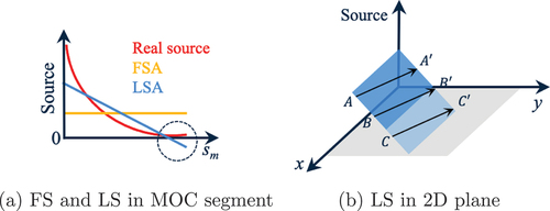
In extreme circumstances, a negative angular flux can be computed due to the negative source caused by the LSA. Figure 3b shows an example of a LS in the 2D plane. Considering the MOC segment $\mathit{AA}{ }^{\mathrm{\prime }}$, the source at every point is positive. In this case, there is no problem. For the case of segment $\mathit{BB}{ }^{\mathrm{\prime }}$, the average source integrated along the segment is positive even though there is a negative part at the end of the segment. However, for the segment $\mathit{CC}{ }^{\mathrm{\prime }}$, a negative source exists at every point on the segment. In this circumstance, the outgoing angular flux can be negative if the incoming angular flux is not sufficiently large to compensate for the negative source. This situation does not make sense physically, and it can lead to unstable iterations.

It is necessary to address this negative source issue to ensure robust and stable convergence. A new method is developed in this work to reduce, or relax, the LS gradient of a problematic cell. We refer to this method as LLSA.

II.B.1. The LLSA for 2D MOC

In the LLSA, the minimum local source ${\bar{q}}_{\mathit{i}}^{\mathit{g},min}$ is computed by Eq. (40)(40) ${\bar{q}}_{\mathit{i}}^{\mathit{g},min}=\underset{\mathit{m},\mathit{k}}{min}\left\{{\bar{q}}_{\mathit{aki}}^{\mathit{g}}\pm {\hat{q}}_{\mathit{mi}}^{\mathit{g}}\frac{{\mathit{t}}_{\mathit{mki}}}{2}\right\}.$(40) :

(40) ${\bar{q}}_{\mathit{i}}^{\mathit{g},min}=\underset{\mathit{m},\mathit{k}}{min}\left\{{\bar{q}}_{\mathit{aki}}^{\mathit{g}}\pm {\hat{q}}_{\mathit{mi}}^{\mathit{g}}\frac{{\mathit{t}}_{\mathit{mki}}}{2}\right\}.$(40)

The minimum value along a segment is at either the entrance or the exit of the segment because the source is linear. Note that in Eq. (40)(40) ${\bar{q}}_{\mathit{i}}^{\mathit{g},min}=\underset{\mathit{m},\mathit{k}}{min}\left\{{\bar{q}}_{\mathit{aki}}^{\mathit{g}}\pm {\hat{q}}_{\mathit{mi}}^{\mathit{g}}\frac{{\mathit{t}}_{\mathit{mki}}}{2}\right\}.$(40) , ${\bar{q}}_{\mathit{aki}}^{\mathit{g}},$ which is defined in Eq. (36)(36) ${\bar{q}}_{\mathit{aki}}^{\mathit{g}}={\bar{q}}_{\mathit{i}}^{\mathit{g}}+{\mathbf{x}}_{aki}^{\mathrm{c}}\cdot {\hat{\mathbf{q}}}_{\mathit{i}}^{\mathit{g}}.$(36) , is used for both P₀ and LIFA sources In other words, only the P₀ component is used in the calculation of Eq. (40)(40) ${\bar{q}}_{\mathit{i}}^{\mathit{g},min}=\underset{\mathit{m},\mathit{k}}{min}\left\{{\bar{q}}_{\mathit{aki}}^{\mathit{g}}\pm {\hat{q}}_{\mathit{mi}}^{\mathit{g}}\frac{{\mathit{t}}_{\mathit{mki}}}{2}\right\}.$(40) regardless of the maximum scattering order. This is intended to prevent the negative source from the P₀ flux and source only. To ensure nonnegativity of the source, we introduce a gradient reduction factor ${\gamma }_i^g$, which is defined as follows:

(41) ${\gamma }_i^g=min\left(\frac{{\bar{q}}_{\mathit{i}}^{\mathit{g}}}{{\bar{q}}_{\mathit{i}}^{\mathit{g}}-{\bar{q}}_{\mathit{i}}^{\mathit{g},min}},1\right).$(41)

When ${\bar{q}}_{\mathit{i}}^{\mathit{g},min}$ is nonnegative, ${\gamma }_i^g$ is unity because it is not necessary to reduce the LS gradient. Conversely, if ${\bar{q}}_{\mathit{i}}^{\mathit{g},min}$ is negative in the first term, the denominator becomes larger than ${\bar{q}}_{\mathit{i}}^{\mathit{g}}.$ Therefore, the range of ${\gamma }_i^g$ is between 0 and 1. When ${\gamma }_i^g$ is equal to 0, the method will be the same as the FSA. To reduce the gradient of the LS, ${\gamma }_i^g$ is multiplied to ${\hat{\mathbf{q}}}_{\mathit{i}}^{\mathit{g}}.$

Mathematically, $\mathit{q}{{\mathit{ }}^{\mathrm{\prime }}}_{\mathit{mki}}^{\mathit{g}}$ in Eq. (18)(18) $q_{mki}^g(\mathit{t})={\bar{q}}_{\mathit{mki}}^{\mathit{g}}+{\hat{q}}_{\mathit{mi}}^{\mathit{g}}\left(\mathit{t}-\frac{{\mathit{t}}_{\mathit{mki}}}{2}\right),$(18) is modified by ${\gamma }_i^g$ as follows:

(42) $\begin{array}{rl}\mathit{q}{{\mathit{ }}^{\mathrm{\prime }}}_{\mathit{mki}}^{\mathit{g}}(\mathit{t})& ={{\bar{q}}^{\prime }}_{\mathit{mki}}^{\mathit{g}}+{{\hat{q}}_{\mathit{ai}}^{\prime }}^{\mathit{g}}\left(\mathit{t}-\frac{{\mathit{t}}_{\mathit{mki}}}{2}\right)\\ \mathit{\hspace{0.17em}}& ={\bar{q}}_{\mathit{mi}}^{\mathit{g}}+{\gamma }_i^g{\mathbf{x}}_{aki}^c\cdot {\hat{\mathbf{q}}}_{\mathit{i}}^{\mathit{g}}+\frac{1}{{\mathit{\xi }}_{\mathit{ai}}}{\gamma }_i^g{\mathbf{\Omega }}_{\mathit{xy},\mathit{m}}\cdot {\hat{\mathbf{q}}}_{\mathit{i}}^{\mathit{g}}\left(\mathit{t}-\frac{{\mathit{t}}_{\mathit{mki}}}{2}\right),\end{array}$(42)

where $(\cdot ){ }^{\mathrm{\prime }}$ indicates the parameter is modified by ${\gamma }_i^g$. Note that ${\bar{q}}_{\mathit{mi}}^{\mathit{g}}$ in Eq. (42)(42) $\begin{array}{rl}\mathit{q}{{\mathit{ }}^{\mathrm{\prime }}}_{\mathit{mki}}^{\mathit{g}}(\mathit{t})& ={{\bar{q}}^{\prime }}_{\mathit{mki}}^{\mathit{g}}+{{\hat{q}}_{\mathit{ai}}^{\prime }}^{\mathit{g}}\left(\mathit{t}-\frac{{\mathit{t}}_{\mathit{mki}}}{2}\right)\\ \mathit{\hspace{0.17em}}& ={\bar{q}}_{\mathit{mi}}^{\mathit{g}}+{\gamma }_i^g{\mathbf{x}}_{aki}^c\cdot {\hat{\mathbf{q}}}_{\mathit{i}}^{\mathit{g}}+\frac{1}{{\mathit{\xi }}_{\mathit{ai}}}{\gamma }_i^g{\mathbf{\Omega }}_{\mathit{xy},\mathit{m}}\cdot {\hat{\mathbf{q}}}_{\mathit{i}}^{\mathit{g}}\left(\mathit{t}-\frac{{\mathit{t}}_{\mathit{mki}}}{2}\right),\end{array}$(42) is simplified to ${\bar{q}}_{\mathit{i}}^{\mathit{g}}$ in the case of P₀ scattering. The LLSA reduces the gradient of the linear component only so that the average source and neutron population are still conserved. This is analogous to maintaining positivity by moving continuously between the full LSA and FSA where only the local spatial discretization error of the source is increased from that of the LSA to that of the FSA at worst. When ${\gamma }_i^g<1$, this is a good indicator that the spatial mesh of the MOC calculation should be refined. Since this is difficult to determine a priori, particularly in a multiphysics problem, the LLSA method provides a robust way to still obtain an answer at an accuracy better than FS MOC.

In our use of LLSA, the emergence of a negative flux or source is not detected if the cell-average source is nonnegative. When the TCP₀ scattering model is used, a negative ${\bar{q}}_{\mathit{i}}^{\mathit{g}}$ can be detected due to the significant negative self-scattering cross section in hydrogen.^[32] However, this issue is not deeply related to the LSA, so its consideration is not treated in this paper.

II.B.2. The LLSA in the 2D/1D Method

The 2D/1D method is one of the feasible solutions for 3D direct whole-core transport calculations. In 2D/1D, the radial direction is solved by the 2D MOC method, and the axial 1D problem is solved by the nodal P₃ (or SP₃) method. The 2D and 1D problems are coupled with the TLs. One of the issues with the 2D/1D method is that the TL is not necessarily positive and the total source is not guaranteed to be positive; therefore, appropriate treatments are necessary. There have been several previous works related to improving or circumventing the stability issues of 2D/1D. These include direct 3D MOC^[10,28] and 2D/3D approaches^[18,33,34] to avoid the stability issues in the 2D/1D method; however, these methods are much more computationally expensive than the 2D/1D method. Other attempts at improving the stability and accuracy of the 2D/1D methods include the TL splitting method^[35] with a proper relaxation factor.^[36] Therefore, this work also focuses on the LSA for the 2D/1D method.

Since the 2D/1D method uses the 2D MOC in the radial direction, the LSA can be easily used for the 2D/1D method. The only difference of the LLSA in the 2D/1D MOC equations is the existence of the TL from the axial nodal solver. With the TL ${\bar{L}}_{\mathit{i}}^{\mathit{g}}$, the transport equation along a segment is written as

(43) $\frac{d{\psi }_{mki}^g(\mathit{t})}{\mathit{dt}}+{\mathrm{\Sigma }}_{t,i}^g{\psi }_{mki}^g(\mathit{t})={\bar{q}}_{\mathit{mki}}^{\mathit{g}}+{\hat{q}}_{\mathit{mi}}^{\mathit{g}}\left(\mathit{t}-\frac{{\mathit{t}}_{\mathit{mki}}}{2}\right)+{\bar{L}}_{\mathit{i}}^{\mathit{g}},$(43)

where

(44) ${\bar{L}}_{\mathit{i}}^{\mathit{g}}=-\frac{{\bar{J}}_{\mathit{i},\mathit{z}+1/2}^{\mathit{g}}-{\bar{J}}_{\mathit{i},\mathit{z}-1/2}^{\mathit{g}}}{4\mathit{\pi }\mathrm{\Delta }{h}_z},$(44)

$\mathrm{\Delta }{h}_z$ = height of plane $\mathit{z}$; ${\bar{J}}_{\mathit{i},\mathit{z}+1/2}^{\mathit{g}}$ and ${\bar{J}}_{\mathit{i},\mathit{z}-1/2}^{\mathit{g}}$ = net current at upper and lower boundaries of plane $\mathit{z}$, respectively.

In the 2D/1D method, a negative flux can be detected because the TL can have a negative value. If there is no constraint to prevent a negative TL, it is possible to encounter a negative source. Therefore, some TL splitting method^[35] is used in most of the codes adopting the 2D/1D method. There are many variations in the TL splitting method depending on how to determine ${\bar{L}}_{\mathit{i}}^{\mathit{g}}$ and ${\bar{J}}_{\mathit{i},\mathit{z}\pm 1/2}^{\mathit{g}},$^[35,37] but the limited flat and isotropic TL is used in this work since it is the default option in MPACT. If a total P₀ source (i.e., ${\bar{q}}_{\mathit{i}}^{\mathit{g}}+{\bar{L}}_{\mathit{i}}^{\mathit{g}}$) calculated based on the solution from the previous iteration or initial guess is less than zero, then a sufficient fraction of the TL source is moved to the left-hand side of the equation with an isotropic flux assumption [i.e., ${\bar{\varphi }}_{\mathit{i}}^{\mathit{g}}\approx 4\mathit{\pi }{\psi }_{mki}^g(\mathit{t})$] as follows:

(45) $\begin{array}{rl}& \frac{d{\psi }_{mki}^g(\mathit{t})}{\mathit{dt}}+\left({\mathrm{\Sigma }}_{t,i}^g-\frac{{\bar{q}}_{\mathit{i}}^{\mathit{g}}+{\bar{L}}_{\mathit{i}}^{\mathit{g}}}{{\bar{\varphi }}_{\mathit{i}}^{\mathit{g}}/4\mathit{\pi }}\right){\psi }_{mki}^g(\mathit{t})\\ & ={\bar{q}}_{\mathit{mki}}^{\mathit{g}}+{\hat{q}}_{\mathit{mi}}^{\mathit{g}}\left(\mathit{t}-\frac{{\mathit{t}}_{\mathit{mki}}}{2}\right)-{\bar{q}}_{\mathit{i}}^{\mathit{g}}\\ & ={\bar{q}}_{\mathit{mi}}^{\mathit{g}}-{\bar{q}}_{\mathit{i}}^{\mathit{g}}+{\mathbf{x}}_{aki}^{\mathrm{c}}\cdot {\hat{\mathbf{q}}}_{\mathit{i}}^{\mathit{g}}+\frac{{\mathbf{\Omega }}_{\mathit{xy},\mathit{m}}\cdot {\hat{\mathbf{q}}}_{\mathit{i}}^{\mathit{g}}}{{\xi }_{\mathit{ai}}}\left(\mathit{t}-\frac{{\mathit{t}}_{\mathit{mki}}}{2}\right).& (45)\end{array}$(45)

In both the FSA and the LSA, the TL splitting is performed with the coarse cell-averaged P₀ source ${\bar{q}}_{\mathit{i}}^{\mathit{g}}$ and TL ${\bar{L}}_{\mathit{i}}^{\mathit{g}}$ regardless of the maximum order of the scattering source. In the case of the FS MOC with the P₀ scattering, the right-hand side of Eq. (45)(45) $\begin{array}{rl}& \frac{d{\psi }_{mki}^g(\mathit{t})}{\mathit{dt}}+\left({\mathrm{\Sigma }}_{t,i}^g-\frac{{\bar{q}}_{\mathit{i}}^{\mathit{g}}+{\bar{L}}_{\mathit{i}}^{\mathit{g}}}{{\bar{\varphi }}_{\mathit{i}}^{\mathit{g}}/4\mathit{\pi }}\right){\psi }_{mki}^g(\mathit{t})\\ & ={\bar{q}}_{\mathit{mki}}^{\mathit{g}}+{\hat{q}}_{\mathit{mi}}^{\mathit{g}}\left(\mathit{t}-\frac{{\mathit{t}}_{\mathit{mki}}}{2}\right)-{\bar{q}}_{\mathit{i}}^{\mathit{g}}\\ & ={\bar{q}}_{\mathit{mi}}^{\mathit{g}}-{\bar{q}}_{\mathit{i}}^{\mathit{g}}+{\mathbf{x}}_{aki}^{\mathrm{c}}\cdot {\hat{\mathbf{q}}}_{\mathit{i}}^{\mathit{g}}+\frac{{\mathbf{\Omega }}_{\mathit{xy},\mathit{m}}\cdot {\hat{\mathbf{q}}}_{\mathit{i}}^{\mathit{g}}}{{\xi }_{\mathit{ai}}}\left(\mathit{t}-\frac{{\mathit{t}}_{\mathit{mki}}}{2}\right).& (45)\end{array}$(45) is zero, so there is no need to consider the negative source issue. In the LSA, however, the source term is not zero. If the TL splitting for the FS is used for the LSA, then cell averaged source (e.g., flat component) is still zero, but this necessarily means that half the LS is positive and the other half is negative across the cell.

There is an alternative choice for splitting the TL, which is to split ${\bar{L}}_{\mathit{i}}^{\mathit{g}}$ when ${\bar{L}}_{\mathit{i}}^{\mathit{g}}$ is negative. In this case, the source term is identical to that of the 2D MOC. However, splitting ${\bar{L}}_{\mathit{i}}^{\mathit{g}}$ instead of splitting the total P₀ source (i.e., ${\bar{q}}_{\mathit{i}}^{\mathit{g}}+{\bar{L}}_{\mathit{i}}^{\mathit{g}}$) introduces a more severe approximation, so it can degrade the accuracy significantly. Since the term that is split is integrated into the total cross section with an isotropic flux approximation, it is necessary to minimize the amount of splitting to reduce the error. For this reason, MPACT splits the total source only if the source is negative. This issue is discussed further in Sec. III.

A new source splitting method in the LLSA is developed to prevent the negative source. In this method, it is necessary to find the minimum source identical to Eq. (40)(40) ${\bar{q}}_{\mathit{i}}^{\mathit{g},min}=\underset{\mathit{m},\mathit{k}}{min}\left\{{\bar{q}}_{\mathit{aki}}^{\mathit{g}}\pm {\hat{q}}_{\mathit{mi}}^{\mathit{g}}\frac{{\mathit{t}}_{\mathit{mki}}}{2}\right\}.$(40) . Note that the gradient reduction factor ${\gamma }_i^g$ has been applied to the terms in Eq. (46)(46) ${{\bar{q}}^{\prime }}_{\mathit{i}}^{\mathit{g},min}=\underset{\mathit{m},\mathit{k}}{min}\left\{{{\bar{q}}^{\prime }}_{\mathit{mki}}^{\mathit{g}}\pm {{\hat{q}}^{\prime }}_{\mathit{mki}}^{\mathit{g}}\frac{{\mathit{t}}_{\mathit{mki}}}{2}\right\}.$(46) :

(46) ${{\bar{q}}^{\prime }}_{\mathit{i}}^{\mathit{g},min}=\underset{\mathit{m},\mathit{k}}{min}\left\{{{\bar{q}}^{\prime }}_{\mathit{mki}}^{\mathit{g}}\pm {{\hat{q}}^{\prime }}_{\mathit{mki}}^{\mathit{g}}\frac{{\mathit{t}}_{\mathit{mki}}}{2}\right\}.$(46)

The value ${{\bar{q}}^{\prime }}_{\mathit{i}}^{\mathit{g},min}$ can be calculated by Eq. (46)(46) ${{\bar{q}}^{\prime }}_{\mathit{i}}^{\mathit{g},min}=\underset{\mathit{m},\mathit{k}}{min}\left\{{{\bar{q}}^{\prime }}_{\mathit{mki}}^{\mathit{g}}\pm {{\hat{q}}^{\prime }}_{\mathit{mki}}^{\mathit{g}}\frac{{\mathit{t}}_{\mathit{mki}}}{2}\right\}.$(46) , but ${{\bar{q}}^{\prime }}_{\mathit{i}}^{\mathit{g},min}$ can be more easily obtained as follows if ${\bar{q}}_{\mathit{i}}^{\mathit{g},min}$ and ${\gamma }_i^g$ are already known:

(47) ${{\bar{q}}^{\prime }}_{\mathit{i}}^{\mathit{g},min}=\left({\bar{q}}_{\mathit{i}}^{\mathit{g},min}-{\bar{q}}_{\mathit{i}}^{\mathit{g}}\right){\gamma }_i^g+{\bar{q}}_{\mathit{i}}^{\mathit{g}}.$(47)

In Eq. (47)(47) ${{\bar{q}}^{\prime }}_{\mathit{i}}^{\mathit{g},min}=\left({\bar{q}}_{\mathit{i}}^{\mathit{g},min}-{\bar{q}}_{\mathit{i}}^{\mathit{g}}\right){\gamma }_i^g+{\bar{q}}_{\mathit{i}}^{\mathit{g}}.$(47) , ${\bar{q}}_{\mathit{i}}^{\mathit{g},min}-{\bar{q}}_{\mathit{i}}^{\mathit{g}}$ corresponds to the gradient of the LS; therefore, ${\gamma }_i^g$ is multiplied with that term. If ${{\bar{q}}^{\prime }}_{\mathit{i}}^{\mathit{g},min}+{\bar{L}}_{\mathit{i}}^{\mathit{g}}\mathit{\hspace{0.17em}}<0$, the TL splitting is performed as follows:

(48) $\begin{array}{rl}& \frac{d{\psi }_{mki}^g(\mathit{t})}{\mathit{dt}}+\left({\mathrm{\Sigma }}_{t,i}^g-\frac{{{\bar{q}}^{\prime }}_{\mathit{i}}^{\mathit{g},min}+{\bar{L}}_{\mathit{i}}^{\mathit{g}}}{{\bar{\varphi }}_{\mathit{i}}^{\mathit{g}}/4\mathit{\pi }}\right){\psi }_{mki}^g(\mathit{t})\\ & ={{\bar{q}}^{\prime }}_{\mathit{mki}}^{\mathit{g}}+{{\hat{q}}^{\prime }}_{\mathit{ai}}^{\mathit{g}}\left(\mathit{t}-\frac{{\mathit{t}}_{\mathit{mki}}}{2}\right)-{{\bar{q}}^{\prime }}_{\mathit{i}}^{\mathit{g},min}\\ & ={\bar{q}}_{\mathit{mi}}^{\mathit{g}}-{{\bar{q}}^{\prime }}_{\mathit{i}}^{\mathit{g},min}+{\gamma }_i^g{\mathbf{x}}_{aki}^{\mathrm{c}}\cdot {{\hat{\mathbf{q}}}^{\prime }}_{\mathit{i}}^{\mathit{g}}\\ & +{\gamma }_i^g\frac{{\mathbf{\Omega }}_{\mathit{xy},\mathit{m}}\cdot {{\hat{\mathbf{q}}}^{\prime }}_{\mathit{i}}^{\mathit{g}}}{{\xi }_{\mathit{ai}}}\left(\mathit{t}-\frac{{\mathit{t}}_{\mathit{mki}}}{2}\right).& (48)\end{array}$(48)

The source term of Eq. (48)(48) $\begin{array}{rl}& \frac{d{\psi }_{mki}^g(\mathit{t})}{\mathit{dt}}+\left({\mathrm{\Sigma }}_{t,i}^g-\frac{{{\bar{q}}^{\prime }}_{\mathit{i}}^{\mathit{g},min}+{\bar{L}}_{\mathit{i}}^{\mathit{g}}}{{\bar{\varphi }}_{\mathit{i}}^{\mathit{g}}/4\mathit{\pi }}\right){\psi }_{mki}^g(\mathit{t})\\ & ={{\bar{q}}^{\prime }}_{\mathit{mki}}^{\mathit{g}}+{{\hat{q}}^{\prime }}_{\mathit{ai}}^{\mathit{g}}\left(\mathit{t}-\frac{{\mathit{t}}_{\mathit{mki}}}{2}\right)-{{\bar{q}}^{\prime }}_{\mathit{i}}^{\mathit{g},min}\\ & ={\bar{q}}_{\mathit{mi}}^{\mathit{g}}-{{\bar{q}}^{\prime }}_{\mathit{i}}^{\mathit{g},min}+{\gamma }_i^g{\mathbf{x}}_{aki}^{\mathrm{c}}\cdot {{\hat{\mathbf{q}}}^{\prime }}_{\mathit{i}}^{\mathit{g}}\\ & +{\gamma }_i^g\frac{{\mathbf{\Omega }}_{\mathit{xy},\mathit{m}}\cdot {{\hat{\mathbf{q}}}^{\prime }}_{\mathit{i}}^{\mathit{g}}}{{\xi }_{\mathit{ai}}}\left(\mathit{t}-\frac{{\mathit{t}}_{\mathit{mki}}}{2}\right).& (48)\end{array}$(48) is always nonnegative if ${\bar{q}}_{\mathit{i}}^{\mathit{g}}$ is nonnegative.

It is also worth mentioning that the LLSA is basically doing the transport calculation by locally mixing the LSA and FSA sources to ensure the nonnegativity. Therefore, the method is no less accurate than the FSA and much closer in accuracy to the LSA. In the case of the 2D/1D calculation, the LLSA additionally adjusts the minimum amount of source split to ensure the nonnegative source. The method effectively makes small trade-offs in local accuracy for the global robustness of the numerical method. Section III.F presents how the LLSA effectively makes the trade-off.

II.B.3. Algorithm

The calculation procedure of the LLSA for the 2D/1D method is summarized in Algorithm 3. The algorithm is written for each MOC transport sweep; therefore, LLSA can be used for both eigenvalue and fixed source problems. Before the transport sweep, the fission source and scattering source are prepared. At Line 4, the minimum LS ${\bar{q}}_{\mathit{i}}^{\mathit{g},min,(\mathrm{\ell })}$ is calculated. If ${\bar{q}}_{\mathit{i}}^{\mathit{g},min,(\mathrm{\ell })}$ is negative, the LS coefficient ${\hat{\mathbf{q}}}_{\mathit{i}}^{\mathit{g},(\mathrm{\ell })}$ is adjusted to reduce the source gradient by ${\gamma }_i^{g,(\mathrm{\ell })}.$ If a problem is 3D and the 2D/1D method is used, additional steps are necessary: ${{\bar{q}}^{\prime }}_{\mathit{i}}^{\mathit{g},min,(\mathrm{\ell })}$ is calculated by Eq. (47)(47) ${{\bar{q}}^{\prime }}_{\mathit{i}}^{\mathit{g},min}=\left({\bar{q}}_{\mathit{i}}^{\mathit{g},min}-{\bar{q}}_{\mathit{i}}^{\mathit{g}}\right){\gamma }_i^g+{\bar{q}}_{\mathit{i}}^{\mathit{g}}.$(47) , and then, the TL splitting is performed for the cell or cells that have a negative value of ${{\bar{q}}^{\prime }}_{\mathit{i}}^{\mathit{g},min,(\mathrm{\ell })}+{\bar{L}}_{\mathit{i}}^{\mathit{g},(\mathrm{\ell })}$. Once the source is corrected not to have a negative value, the 2D MOC sweep is performed for all axial planes. The 2D MOC sweep in Line 13 corresponds to the first for loop in Algorithm 1 (Line 4) or Algorithm 2 (Line 3) depending on the source type in these algorithms.

Algorithm 3 LLSA algorithm for each MOC transport sweep

1: Prepare ${\bar{\varphi }}_{\mathit{i}}^{\mathit{g},(\mathrm{\ell })}$ and ${\hat{\varphi }}_{\mathit{i}}^{\mathit{g},(\mathrm{\ell })}$ from previous sweep or initial guess

2: for Region $\mathit{i}$ and energy groups $\mathit{g}$ do

3:     Calculate ${\hat{\mathbf{q}}}_{\mathit{i}}^{\mathit{g},(\mathrm{\ell })}$ in Eq. (12)(12) ${\hat{\mathbf{q}}}_{\mathit{i}}^{\mathit{g}}=\frac{1}{4\mathit{\pi }}\left[\sum _{\mathit{g}{\mathit{ }}^{\mathrm{\prime }}}{\mathrm{\Sigma }}_{\mathit{s},\mathit{i}}^{\mathit{g}{\mathit{ }}^{\mathrm{\prime }}\to \mathit{g}}{\widehat{\text{phii}}}_{\mathit{i}}^{\mathit{g}{ }^{\mathrm{\prime }}}+\frac{{\chi }_i^g}{k_{\mathrm{eff}}}\sum _{\mathit{g}{\mathit{ }}^{\mathrm{\prime }}}\mathit{\nu }{\mathrm{\Sigma }}_{\mathit{f},\mathit{i}}^{\mathit{g}{\mathit{ }}^{\mathrm{\prime }}}{\widehat{\text{phii}}}_{\mathit{i}}^{\mathit{g}{ }^{\mathrm{\prime }}}\right],$(12)

4:     Calculate ${\bar{q}}_{\mathit{i}}^{\mathit{g},min,(\mathrm{\ell })}$ in Eq. (40)(40) ${\bar{q}}_{\mathit{i}}^{\mathit{g},min}=\underset{\mathit{m},\mathit{k}}{min}\left\{{\bar{q}}_{\mathit{aki}}^{\mathit{g}}\pm {\hat{q}}_{\mathit{mi}}^{\mathit{g}}\frac{{\mathit{t}}_{\mathit{mki}}}{2}\right\}.$(40)

5:     Calculate ${\gamma }_i^{g,(\mathrm{\ell })}$ in Eq. (41)(41) ${\gamma }_i^g=min\left(\frac{{\bar{q}}_{\mathit{i}}^{\mathit{g}}}{{\bar{q}}_{\mathit{i}}^{\mathit{g}}-{\bar{q}}_{\mathit{i}}^{\mathit{g},min}},1\right).$(41)

6:     Multiply ${\gamma }_i^{g,(\mathrm{\ell })}$ to ${\hat{\mathbf{q}}}_{\mathit{i}}^{\mathit{g},(\mathrm{\ell })}$

7:     if 2D/1D method is used then

8:         Calculate ${{\bar{q}}^{\prime }}_{\mathit{i}}^{\mathit{g},min,(\mathrm{\ell })}$ in Eq. (47)(47) ${{\bar{q}}^{\prime }}_{\mathit{i}}^{\mathit{g},min}=\left({\bar{q}}_{\mathit{i}}^{\mathit{g},min}-{\bar{q}}_{\mathit{i}}^{\mathit{g}}\right){\gamma }_i^g+{\bar{q}}_{\mathit{i}}^{\mathit{g}}.$(47)

9:         Obtain ${\bar{L}}_{\mathit{i}}^{\mathit{g},(\mathrm{\ell })}$ in Eq. (44)(44) ${\bar{L}}_{\mathit{i}}^{\mathit{g}}=-\frac{{\bar{J}}_{\mathit{i},\mathit{z}+1/2}^{\mathit{g}}-{\bar{J}}_{\mathit{i},\mathit{z}-1/2}^{\mathit{g}}}{4\mathit{\pi }\mathrm{\Delta }{h}_z},$(44) from 1D axial nodal solver

10:         Perform TL splitting in Eq. (48)(48) $\begin{array}{rl}& \frac{d{\psi }_{mki}^g(\mathit{t})}{\mathit{dt}}+\left({\mathrm{\Sigma }}_{t,i}^g-\frac{{{\bar{q}}^{\prime }}_{\mathit{i}}^{\mathit{g},min}+{\bar{L}}_{\mathit{i}}^{\mathit{g}}}{{\bar{\varphi }}_{\mathit{i}}^{\mathit{g}}/4\mathit{\pi }}\right){\psi }_{mki}^g(\mathit{t})\\ & ={{\bar{q}}^{\prime }}_{\mathit{mki}}^{\mathit{g}}+{{\hat{q}}^{\prime }}_{\mathit{ai}}^{\mathit{g}}\left(\mathit{t}-\frac{{\mathit{t}}_{\mathit{mki}}}{2}\right)-{{\bar{q}}^{\prime }}_{\mathit{i}}^{\mathit{g},min}\\ & ={\bar{q}}_{\mathit{mi}}^{\mathit{g}}-{{\bar{q}}^{\prime }}_{\mathit{i}}^{\mathit{g},min}+{\gamma }_i^g{\mathbf{x}}_{aki}^{\mathrm{c}}\cdot {{\hat{\mathbf{q}}}^{\prime }}_{\mathit{i}}^{\mathit{g}}\\ & +{\gamma }_i^g\frac{{\mathbf{\Omega }}_{\mathit{xy},\mathit{m}}\cdot {{\hat{\mathbf{q}}}^{\prime }}_{\mathit{i}}^{\mathit{g}}}{{\xi }_{\mathit{ai}}}\left(\mathit{t}-\frac{{\mathit{t}}_{\mathit{mki}}}{2}\right).& (48)\end{array}$(48) if $({{\bar{q}}^{\prime }}_{\mathit{i}}^{\mathit{g},min,(\mathrm{\ell })}+{\bar{L}}_{\mathit{i}}^{\mathit{g},(\mathrm{\ell })})<0$

11:     end if

12: end for

13: Perform 2D MOC sweep for all $\mathit{z}$

III. NUMERICAL RESULTS

The accuracy and the computational performance of the LSA in MPACT are examined in this section. The method is verified against the C5G7 benchmark, PWR, and boiling water reactor (BWR) problems. Results on the validation of the LS have been presented in previous work.^[38] This work focuses on the performance and relative accuracy based on discretization parameters.

In the following sections, the solution from FSA and LSA is compared to a reference that uses a very fine mesh discretization for the LSA MOC and spatial discretization, except for the C5G7 benchmark, which has a reference Monte Carlo solution. The fine mesh reference solution is generated so that the error we expect from the spatial discretization is less than 10 pcm $\mathrm{\Delta k}$ and 0.05% root-mean-square (RMS) in the pin power distribution compared to some ultrafine mesh. By doing this, the error from the cross-section calculation method can be neglected, and the resulting differences can be assumed to depend only on the spatial mesh discretization and source approximation. In most of the comparisons, two additional mesh discretization methods are used: medium mesh and coarse mesh. The notations for each method are the following:

1. FS-Medium: Medium mesh with FSA.

2. LS-Medium: Medium mesh with LSA.

3. FS-Coarse: Coarse mesh with FSA.

4. LS-Coarse: Coarse mesh with LSA.

The medium mesh is the mesh that is reasonably fine so that the FS MOC with the medium mesh may calculate acceptable solutions in a practical calculation. The acceptable criteria may depend on many factors (i.e., problem applications and a purpose of analysis). In this paper, the target accuracy is less than 50 pcm eigenvalue error and less than 0.1% RMS pin power error, which is well below what is suggested for high-fidelity analysis in Ref. [39]. The coarse mesh is a transport discretization coarser than the medium mesh. When used with LSA, it is intended to correspond to the level of accuracy of the medium mesh with FSA. It is expected that the coarse mesh with FSA does not provide a sufficiently accurate solution. The meshing methods for fine, medium, and coarse meshes are described in each section since they depend on problem cases. In each subsection, the relative MOC run time is compared. It should be noted that the relative MOC run time is the run time used in the MOC eigenvalue calculation to focus on only the computational efficiency of the MOC schemes. Therefore, the run time does not include the time spent in the initialization, cross-section calculation, CMFD solver, etc.

III.A. C5G7 Benchmark

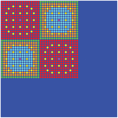
The 2D C5G7 benchmark^[40] is a neutronics benchmark used by various codes to help verify the correctness of the solvers used. A seven-group cross-section library of macroscopic cross sections is provided by the benchmark. The benchmark consists of two uranium oxide (UO₂) assemblies and two mixed oxide (MOX) assemblies surrounded by a large radial reflector, as shown in Fig. 4. Reflective boundary conditions are used on the north and west faces while vacuum conditions are used on the south and east faces. The benchmark provides a reference MCNP Monte Carlo result that can be used to determine the accuracy of other methods used to solve the benchmark cases.

Fig. 4. Geometry and materials of the 2D C5G7 benchmark.

All cases used a uniform ray spacing of 0.05 cm and directional quadrature using 128 azimuthal angles and six polar angles in $4\mathit{\pi }$. Each case was run using an optimally diffusive Coarse Mesh Finite Difference method.^[41] Table I presents the mesh options for the medium and coarse mesh cases. The medium pin cell mesh used 3 fuel radial rings with 8 azimuthal divisions, and 4 radial regions with 16 azimuthal divisions in the moderator. The medium reflector cell mesh was divided into 0.105 $\times$ 0.105 cm², which corresponds to 12 $\times$ 12 divisions in the reflector unit cell. The coarse pin cell mesh used a single fuel ring with four azimuthal divisions and one radial moderator region using eight azimuthal divisions. The coarse reflector cell mesh was divided into 0.42- $\times$ 0.42-cm² cells. The Table II segments show the relative number of source regions and MOC segments of two meshes. The coarse mesh uses 9% and 30% number of source regions and MOC segments, respectively, compared to that of the medium mesh case.

TABLE I Mesh Options for the 2D C5G7 Benchmark

Parameters		Medium Mesh	Coarse Mesh
Fuel unit cell^a	Rod	3/8	1/4
	Coolant	4/16	1/8
Reflector unit cell^b		12$\times$12	3$\times$3

^aNumberof radial divisions/number of azimuthal divisions.

^bNumber of divisions in the $\mathit{x}$-direction $\times$ number of divisions in the $\mathit{y}$-direction.

TABLE II The Relative Number of Source Regions and MOC Segments of C5G7 Problem

Source Regions (Coarse/Medium)	MOC Segments (Coarse/Medium)
0.09	0.30

It is expected that the LS-Coarse case should reduce run time while maintaining accuracy compared to the FS-Medium calculation. Additionally, the FS-Coarse calculation should have worse accuracy, thus justifying the use of the LSA.

Table III shows very clearly that the LS-Coarse case is more accurate than FS-Coarse. While FS-Medium provides reasonable accuracy, FS-Coarse shows significant differences compared to the Monte Carlo reference. In terms of the RMS pin power difference, the LSA is six times more accurate than the FSA. The LSA cases have 0.13% RMS pin power differences that are within the RMS standard deviation of the solution. Since there is no noticeable difference between LS-Coarse and LS-Medium, it can be assumed that the coarse mesh is sufficiently refined to have high accuracy with the LSA for the C5G7 benchmark.

TABLE III Accuracy Comparisons for the C5G7 2D Benchmark Calculation Using Different Source Approximations and Meshes

Method	$\mathrm{\Delta }$$k_{\mathit{eff}}$ (pcm)^a	Pin Power Difference (%)
		RMS^b	Maximum
FS-Medium	2	0.19	0.76
LS-Medium	−7	0.13	0.50
FS-Coarse	65	0.81	2.19
LS-Coarse	−3	0.13	0.49

^aThe reference eigenvalue statistical error is $\pm$5 pcm.

^bThe reference RMS pin power statistical error is $\pm$0.14%.

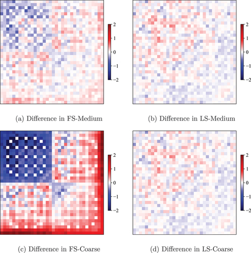
The pin power differences of each case are visualized in Fig. 5. The largest pin power differences for FS-Medium, LS-Medium, and LS-Coarse are in the center assembly where pin powers are higher. On the other hand, the FS-Coarse case has significant pin power difference in the pins bordering the radial reflector region. This indicates that the mesh in the reflector is not sufficient to capture the spatial gradients of the source. The differences in the interior of the assemblies are still larger for this case than the others.

Fig. 5. C5G7 problem pin power differences (in units of percent).

The run-time and memory results are presented in Table IV. The results of each case are normalized to the results of the FS-Medium case to easily estimate run time and memory overhead. Table IV indicates that the LS-Coarse case significantly outperforms FS-Medium. The MOC run time per iteration is reduced by 46%, and memory usage is reduced by 15%. The numbers of iterations to converge each case are slightly different. However, the numbers of iterations from the FSA and LSA are the same when solving multistate problems that reactor analysts are normally interested in. This is further discussed in Sec. III.D. As a result of the slight variation in iterations between the cases, the run time per iteration is mainly used when comparing the run-time performance in the rest of this paper. Table IV also shows that for this problem, the LS-Coarse case takes about 1.69 times the time of FS-Coarse. The LS-Coarse method uses 20% more memory than FS-Coarse.

TABLE IV Performance Comparisons for the C5G7 2D Benchmark Calculation Using Different Source Approximations and Meshes

Method	Relative Iterations	Relative MOC Run Time/Iteration	Relative Memory
FS-Medium	1.00	1.00	1.00
LS-Medium	1.06	2.04	3.26
FS-Coarse	0.89	0.32	0.71
LS-Coarse	1.06	0.54	0.85

Generally, the LS MOC solver is 1.4 to 2.1 times slower than the FS MOC solver with the same mesh. The run-time overhead depends on several factors such as energy groups, mesh, MOC rays, computer hardware, and compiler options for optimization. The 1.69 times run-time overhead of the LSA was calculated with the GNU compiler using the −O3 optimization option. However, the run-time overhead can be improved to 1.4 with more aggressive optimizations that use the −O3 − march = native options. For consistency, all calculation results in this paper are based on the default compiler options in MPACT, which is −O3 (for GCC-5.4.0). We mention these details for comparison to the LSA method in CASMO5, which is 1.55 times slower than the FSA for the C5G7 benchmark with coarse mesh.^[9] We also mention that it is not proper to conclude that the LSA in MPACT is strictly slower or faster than the LSA in CASMO5 since the tests were not performed in the same environment and only relative increases in run time are reported. Nevertheless, the authors assert that the LSA in MPACT is computationally more efficient for multiphysics and 2D/1D calculations due to the reformulation of the method and because the LSA methods in both codes have a similar average segment integration time for 2D lattice single physics calculations.^[25]

For the medium mesh cases, the LS-Medium case is 2 times slower, and it uses more than 3 times larger memory than the FS-Medium case. The 3 times larger overhead of the memory is not typical for the practical calculations used in design and analysis. The medium mesh case of the C5G7 benchmark uses a large number of mesh for the coolant and reflector regions due to finely refined mesh as described in Table I. A typical LWR problem does not need this amount of discretization. In addition, the C5G7 benchmark cross section uses only seven energy groups while the typical number of energy groups in the transport calculation is several tens to hundreds.

The energy-independent geometry data take up a large portion of memory for this specific case because of these two reasons. Specifically, ${\xi }_{\mathit{ai}}$ in Eq. (5)(5) ${\xi }_{\mathit{ai}}=\frac{V_i}{{\sum }_k\mathit{\delta }{A}_a{s}_{\mathit{mki}}}.$(5) , ${\mathbf{X}}_{ai}^{\mathrm{c}}$ in Eq. (7)(7) ${\mathbf{X}}_{ai}^c={⟨\mathbf{X}⟩}_{\mathit{mi}}.$(7) , and ${\mathbf{M}}_i$ in Eq. (15)(15) $\begin{array}{rl}& {\mathbf{M}}_i=\frac{1}{4\mathit{\pi }}{⟨\mathbf{x}{\mathbf{x}}^T⟩}_{\mathit{i}}=\frac{1}{4\pi V_i}\sum _m{\omega }_m\sum _k\mathit{\delta }{A}_{a}sin{\theta }_p{t}_{\mathit{mki}}\\ & {⟨\left({\mathbf{x}}_{aki}^{\mathrm{i}\mathrm{n}}+{\mathbf{\Omega }}_{\mathit{xy},\mathit{m}}\mathit{t}/{\xi }_{\mathit{ai}}\right){\left({\mathbf{x}}_{aki}^{\mathrm{i}\mathrm{n}}+{\mathbf{\Omega }}_{\mathit{xy},\mathit{m}}\mathit{t}/{\xi }_{\mathit{ai}}\right)}^{\mathit{T}}⟩}_{\mathit{mki}}\\ & =\frac{1}{4\pi V_i}\sum _m{\omega }_m\sum _k\mathit{\delta }{A}_{a}sin{\theta }_p{t}_{\mathit{mki}}\\ & \left[{\mathbf{x}}_{aki}^c{\left({\mathbf{x}}_{aki}^c\right)}^{\mathit{T}}+\frac{{{\mathit{t}}_{\mathit{mki}}}^2}{12{{\mathit{\xi }}_{\mathit{ai}}}^2}{\mathbf{\Omega }}_{\mathit{xy},\mathit{m}}{{\mathbf{\Omega }}_{\mathit{xy},\mathit{m}}}^{\mathit{T}}\right],& (15)\end{array}$(15) for the LSA require a large amount of memory. However, the memory used for these parameters is not dominant in many cases including the LS-Coarse case. Comparing the FS-Coarse and LS-Coarse cases in Table IV shows that the memory overhead is 20%. The memory overhead will decrease further when using many energy groups; results are presented in the next few sections. There may be an alternative way to reduce memory usage in the LSA. The memory for angle-dependent parameters ${\xi }_{\mathit{ai}}$ and ${\mathbf{X}}_{ai}^{\mathrm{c}}$ can be reduced by using the isotropic renormalization in the case of the P₀ scattering case. However, these authors believe that memory does not matter in general; therefore, the angle-dependent renormalization is used in the rest of the paper.

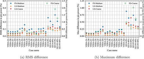
III.B. 2D Fuel Assembly Problems

In this section, PWR and BWR single-assembly problems are tested. The VERA problem 2 cases^[42] have 17 fuel assembly types that have a wide range of fuel enrichment and various burnable absorbers and other inserts. Each case is described in detail in Ref. [42]. For the BWR problems, the GE14 fuel assembly problem^[43] was selected in this test. The BWR progression problem^[43] has two different GE14 fuel lattices with and without vanished rods that induce a sharp flux gradient and make a problem more difficult. The GE14 assembly has a wide range of enrichments and significant numbers of gadolinia rods to control the excess reactivity. The GE14 problem is also simulated at three different void fractions from 0% to 80%. All cases used the 51-energy-group cross-section library, which is based on ENDF-VII.1.^[44]

Each lattice case was run with medium and coarse meshes with the FS MOC and LS MOC solvers. Each of these cases used the Tabuchi-Yamamoto angular quadrature set^[45] with 64 azimuthal angles, 4 polar angles over $4\mathit{\pi }$, and 0.05-cm ray spacing. However, because of thin regions from integral fuel burnable absorber (IFBA) and wet annular burnable adsorber (WABA) rods in cases 2L, 2M, and 2N, a ray spacing of 0.001 cm was used. The results are compared against a very finely meshed case run using the LS MOC solver with 128 azimuthal angles, 4 polar angles, and 0.001-cm ray spacing.

Table V summarizes the mesh options for the fine, medium, and coarse mesh cases. The mesh options are described for some important geometries (i.e., pellet, cladding, and coolant). The fuel pellet and gadolinia have additional radial divisions to accurately capture the flux distribution as well as the burnup distribution throughout the depletion. The radial division in the fine and medium mesh cases is made to have the same volume between the submeshes. The coarse mesh has two radial divisions with a fractional radius of 0.875 for the UO₂ pellet. This fraction was selected from sensitivity tests to accurately capture the rim effect.^[25]

TABLE V Mesh Options for the 2D Fuel Assembly Problems

Parameters		Fine Mesh	Medium Mesh	Coarse Mesh
Fuel unit cell^a	UO2 pellet	15/32	3/8	2/1
	Gadolinia pellet	15/32	10/8	10/1
	Cladding	10/32	1/8	1/1
	Other annulus	1/32	1/8	1/1
	Coolant (PWR)	16/32	2/8	1/4
	Coolant (BWR)	16/32	6/32	2/8
BWR assembly gap unit cell^b		13$\times$10	5$\times$3	4$\times$3
Reflector unit cell^c		12$\times$12	4$\times$4	2$\times$2

^aNumber of radial divisions/number of azimuthal divisions.

^bNumber of divisions parallel to channel box/number of divisions perpendicular to channel box.

^cNumber of divisions in the $\mathit{x}$-direction $\times$ number of divisions in the $\mathit{y}$-direction.

The options for the other cylindrical or annulus geometries (i.e., fuel gap, guide tube, Pyrex, IFBA, and WABA) correspond to “Other annulus” in Table V. The coolant mesh options are provided depending on the reactor types since BWRs generally have a more complicated and heterogeneous design than that of PWRs. For BWR modeling, MPACT generates an additional unit pin cell for the interassembly gap regions since the gap size is pretty large while the gap region is merged to the neighboring fuel unit cell in the PWR applications. The BWR interassembly gap comprises an inner water gap, channel box, and outer water gap. The reflector is not used in these fuel assembly problems, but it is described here for later use in Sec. III.C.

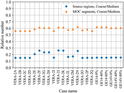
Figure 6 presents the number of source regions and MOC segments of each problem in terms of the ratios of the two meshes. In the figures, VERA-2A to VERA-2Q denote the VERA single-assembly problems in Ref. [42]. The GE14 BWR assemblies with various void fraction percentages are also listed in the figures. Note that the GE14V indicates the GE14 assembly with vanished rods. The medium mesh has more source regions and MOC segments. On average, the coarse transport mesh uses only 18% of source regions and 59% of MOC segments compared to that of the medium mesh.

Fig. 6. The relative number of source regions and MOC segments.

All problems in this section were calculated with the TCP₀ and P₂ scattering options. The TCP₀ scattering may be used in a practical calculation while the P₂ scattering is normally used when higher accuracy is desired. In the comparison, the TCP₀ cases are compared to the reference solution generated with the TCP₀ scattering. Similarly, the P₂ cases are compared to the reference solution with P₂ since the focus of this paper is the accuracy and performance of the LSA instead of the accuracy comparison between TCP₀ and P₂. The reference solutions were calculated with the LS MOC solver, very fine mesh, and a very dense MOC ray spacing and quadrature.

The results for the TCP₀ scattering are summarized in Figs. 7 and 8. It should be noted that results for the FS-Coarse case are presented on a different axis since the order of difference is significantly different from the other cases. The case-averaged results are summarized in Table VI. The results with P₂ scattering are shown in Figs. 9 and 10 and Table VII. The results clearly present that the LSA calculates a more accurate eigenvalue and pin power distribution compared to the FSA. In terms of the RMS pin power difference, the LSA is two to three times more accurate compared with the FS-medium mesh cases irrespective of scattering order. For the coarse mesh, the LSA is 6.6 to 7 times more accurate than the FSA results. Furthermore, the LS-Coarse case is 1.6 to 2 times more accurate than the FS-Medium case. Overall, the LSA calculates more consistent eigenvalue and pin power results across these lattice cases. The FS-Coarse case has very large differences for BWR problems especially for the GE14-0% problem that has a softer spectrum. It is likely that the LSA is essential for BWRs since a BWR assembly design has a more heterogeneous fuel and geometry configuration with a significant amount of gadolinia and the interassembly gap.

TABLE VI Case-Averaged Differences for Eigenvalue and Pin Power Distribution with TCP₀ Scattering

Method	Case-Averaged $\mathrm{\Delta }{k}_{\mathit{eff}}$ (pcm)	Case-Averaged Pin Power Difference (%)
		RMS	Maximum
FS-Medium	39	0.08	0.21
LS-Medium	23	0.04	0.13
FS-Coarse	163	0.33	0.71
LS-Coarse	24	0.05	0.16

TABLE VII Case-Averaged Difference for Eigenvalue and Pin Power Distribution with P₂ Scattering

Method	Case-Averaged $\mathrm{\Delta }{k}_{\mathit{eff}}$ (pcm)	Case-Averaged Pin Power Difference (%)
		RMS	Maximum
FS-Medium	40	0.12	0.27
LS-Medium	22	0.04	0.13
FS-Coarse	158	0.42	0.91
LS-Coarse	34	0.06	0.19

Fig. 7. Eigenvalue difference (compared to fine mesh case) for TCP₀ scattering.

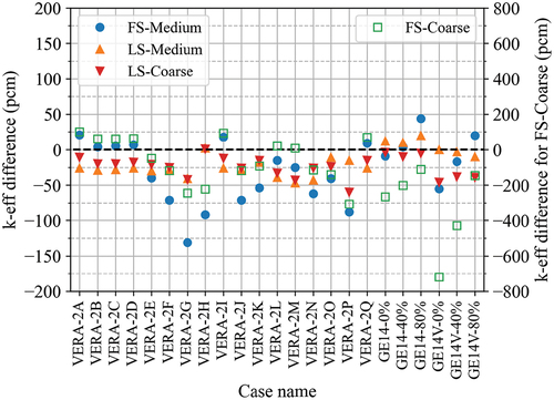
Fig. 8. Pin power difference (compared to fine mesh case) for TCP₀ scattering.

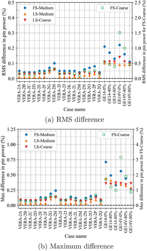
Fig. 9. Eigenvalue difference compared to fine mesh calculation with P₂ scattering.

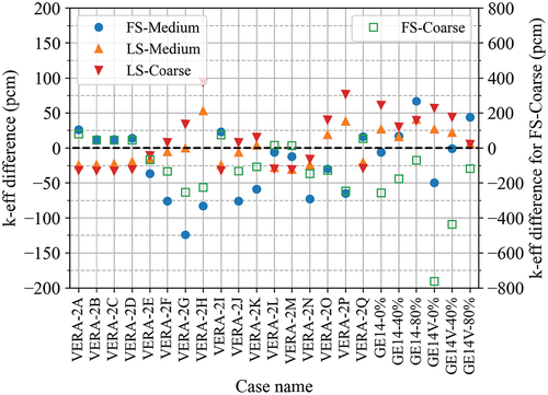
Fig. 10. Difference in pin power compared to fine mesh calculation with P₂ scattering.

Overall, the RMS pin power differences of P₂ cases are 1.2 to 1.5 times larger than that of TCP₀. In general, the transport-corrected total cross section is smaller than the noncorrected total cross section, which is used in the P₂ case. Therefore, the TCP₀ cases may have a longer mean free path. On the other hand, the P₂ cases may have a larger total cross section than that of TCP₀; therefore, the problem becomes more difficult to get a spatially converged solution with the same mesh. It is also worth noting that the LIFA source approximation may have a potential error from the FSA for the higher-order source even though it is hardly noticeable with conventional LWR applications as shown in this section.

The run-time and memory results for the TCP₀ and P₂ cases are presented in Tables VIII and IX. With the same coarse mesh, the LS-Coarse case has a 67% slower run time and 3% more memory usage than the FS-Coarse case for the TCP₀ cases. By comparing LS-Coarse to FS-Medium, LS-Coarse took 12% more time per iteration and used 12% less memory. Even though LS-Coarse is slightly slower than FS-Medium, there is a possibility to make the LS-Coarse case faster than FS-Medium by using coarser mesh than the one used in the test since LS-Coarse is 1.6 to 2 times more accurate than the FS-Medium mesh in terms of the RMS pin power difference.

TABLE VIII Case-Averaged Relative Run Time and Memory with TCP₀ Scattering

Method	Relative Iterations	Relative MOC Run Time/Iteration	Relative Memory
FS-Medium	1.00	1.00	1.00
LS-Medium	1.04	1.90	1.12
FS-Coarse	0.90	0.67	0.85
LS-Coarse	1.05	1.12	0.88

TABLE IX Case-Averaged Relative Run Time and Memory with P₂ Scattering

Method	Relative Iterations	Relative MOC Run Time/Iteration	Relative Memory
FS-Medium	1.00	1.00	1.00
LS-Medium	1.22	1.70	1.08
FS-Coarse	1.01	0.44	0.70
LS-Coarse	1.24	0.79	0.71

The LSA has better performance in the case of anisotropic scattering. In Table IX, LS-Coarse is 21% faster and uses 29% less memory than FS-Medium. As mentioned in Sec. II, the LSA in MPACT uses LIFA. In the LIFA source, the higher-order source moment is spatially flat while the isotropic source is linear. Therefore, the run-time and memory burden to calculate the higher-order flux and source is small in the case of LS-Coarse thanks to the coarse mesh. In general, the high-order flux is spatially more smooth than the P₀ flux. Therefore, the LIFA method is still accurate, and it is possible to take advantage of this fact to have better performance.

III.C. 2D PWR Core Problem

In this section, the VERA-5A 2D core quarter-core problem is evaluated. The specification for the problem is described in Ref. [42]. This problem has quarter-core symmetry so that this problem can be used for the whole-core calculation, which is the main interest of MPACT. The spatial discretizations for the coarse mesh and medium mesh pin cells are the same as described in Table V. The medium reflector cell mesh was divided into approximately 0.316- $\times$ 0.316-cm² cells while the coarse reflector cell mesh was divided into approximately 0.632- $\times$ 0.632-cm² cells. The medium mesh uses five times as many regions as the coarse mesh. The reference solution was calculated with the LS MOC solver, fine mesh, and dense MOC ray spacing and quadrature. In total, 16 distributed memory processors with the same spatial partitioning are used in each simulation.

The eigenvalue and pin power results are presented in Tables X and XI. The pin power differences for the P₂ cases are visualized in the Fig. 11 pin power difference. Similar to the single-assembly problems, both the FS-Medium case and the LS-Coarse case calculate reasonably accurate eigenvalues and pin power distributions. The LS-Coarse case has a 1.6 to 1.7 times more accurate result in terms of RMS pin power difference compared to the FS-Medium case. The FS-Coarse case shows a significant power tilt across the core as shown in Fig. 11c. This power tilt is not observed with the LS-Coarse mesh. The LS-Coarse case is 11 times more accurate in terms of the RMS pin power compared with the FS-Coarse case.

TABLE X VERA-5A 2D Core Problem Eigenvalue and Pin Power Results with TCP₀

Method	$\mathrm{\Delta }$$k_{\mathit{eff}}$ (pcm)	Pin Power Difference (%)
		RMS	Maximum
FS-Medium	−47	0.08	0.25
LS-Medium	−43	0.05	0.11
FS-Coarse	−57	0.58	1.39
LS-Coarse	−32	0.05	0.15

TABLE XI VERA-5A 2D Core Problem Eigenvalue and Pin Power Results with P₂

Method	$\mathrm{\Delta }$$k_{\mathit{eff}}$ (pcm)	Pin Power Difference (%)
		RMS	Maximum
FS-Medium	−44	0.12	0.34
LS-Medium	−29	0.07	0.18
FS-Coarse	−82	0.74	1.73
LS-Coarse	−23	0.07	0.21

Fig. 11. VERA-5A 2D core problem pin power differences with P₂ (in units of percent).

The run-time and memory results are shown in Tables XII and XIII. For the TCP₀ case, the LS-Coarse case is 6% slower but uses 19% less memory than the FS-Medium case. Since the LS-Coarse case has higher accuracy than the FS-Medium case, it is likely that the LS-Coarse case can outperform the FS-Medium case if meshing methods are adjusted to have the same accuracy. The relative memory footprints are shown in the tables, but it is sometimes important to observe the absolute value as well. The total memory requirements in the simulation with TCP₀ are 20.6, 24.7, 15.6, and 16.6 Gbytes for the FS-Medium, LS-Medium, FS-Coarse, and LS-Coarse cases, respectively.

TABLE XII VERA-5A 2D Core Problem Relative Run Time and Memory with TCP₀

Method	Relative Iterations	Relative MOC Run Time/Iteration	Relative Memory
FS-Medium	1.00	1.00	1.00
LS-Medium	1.00	1.97	1.20
FS-Coarse	1.00	0.60	0.76
LS-Coarse	1.00	1.06	0.81

TABLE XIII VERA-5A 2D Core Problem Relative Run Time and Memory with P₂

Method	Relative Iterations	Relative MOC Run Time/Iteration	Relative Memory
FS-Medium	1.00	1.00	1.00
LS-Medium	1.07	1.68	1.12
FS-Coarse	1.00	0.41	0.56
LS-Coarse	1.00	0.69	0.59

The LS-Coarse case with P₂ scattering is 31% faster and uses 41% less memory than FS-Medium with P₂. On the same coarse mesh, the LS-Coarse case is 1.7 times slower and uses 5% to 6% more memory than the FS-Coarse case. It is also noted that the number of iterations is identical for all cases. This is likely because the spatial moment of the LSA does not noticeably degrade the fission source convergence rate in the larger core problem.

III.D. 2D Lattice Depletion

In Sec. III.B, the LS MOC on the coarse mesh was shown to be sufficiently accurate for an array of lattice problems with single physics. Two of these PWR problems, 2A and 2P, were selected for further study by performing isotopic depletion up to 70 MWd/kg HM at HFP conditions. Problem 2A represents a typical lattice configuration consisting of only fuel rods and empty guide tubes. Problem 2P contains several gadolinia rods that act as burnable absorbers; reactivity is significantly damped at the beginning of cycle but increases as gadolinia is burned. The gadolinia rods require significant radial meshing to accurately capture the complicated spatial burnup distributions throughout the depletion (it is effectively a moving boundary layer). As described in Table V, the meshing has 10 equal volume rings in the gadolinia fuel. Because of this complicated distribution, the LS MOC solver cannot eliminate the additional radial rings to maintain the same level of accuracy as the FS MOC solver on the current default mesh. However, similar azimuthal coarsening is possible on these rods, with a single azimuthal region in all but the surrounding coolant, which has four azimuthal regions.

The eigenvalue and pin power results are presented in Figs. 12 and 13. Tables XIV and XV present the burnup-averaged differences in the eigenvalue and pin power distribution. Again, it should be noted that the TCP₀ cases are compared to the fine mesh calculation with TCP₀ while the P₂ cases are compared to the fine mesh with P₂ scattering. For these depletion problems, the LS cases and the FS-Medium case have accurate results with less than 50 pcm difference in the eigenvalue and less than 0.1% in the RMS pin power difference. The FS-Coarse case has larger differences due to spatial discretization error.

TABLE XIV Burnup-Averaged Eigenvalue and Pin Power Differences for VERA 2A Depletion Problem

Method	Scattering	$\mathrm{\Delta }$$k_{\mathit{eff}}$ (pcm)	Pin Power Difference (%)
			RMS	Maximum
FS-Medium	TCP0	21	0.06	0.13
LS-Medium		40	0.05	0.12
FS-Coarse		29	0.10	0.20
LS-Coarse		27	0.06	0.17
FS-Medium	P2	11	0.06	0.14
LS-Medium		30	0.04	0.12
FS-Coarse		38	0.13	0.26
LS-Coarse		23	0.06	0.16

TABLE XV Burnup-Averaged Eigenvalue and Pin Power Differences for VERA 2P Depletion Problem

Method	Scattering	$\mathrm{\Delta }$$k_{\mathit{eff}}$ (pcm)	Pin Power Difference (%)
			RMS	Maximum
FS-Medium	TCP0	19	0.06	0.14
LS-Medium		33	0.04	0.12
FS-Coarse		89	0.16	0.39
LS-Coarse		23	0.05	0.15
FS-Medium	P2	17	0.07	0.15
LS-Medium		32	0.05	0.14
FS-Coarse		76	0.20	0.45
LS-Coarse		35	0.07	0.19

Fig. 12. VERA 2A depletion problem results.

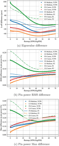
Fig. 13. VERA 2P depletion problem results.

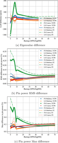
One noticeable result is that the LS cases and the FS-Medium case have very similar accuracy. There are two possible sources of error in interpreting these depletion problems. First, as in the previous section, flux or power results may not be accurate due to insufficient mesh and source representation. Second, there could be an error in the burnup distribution due to an insufficient number of fuel radial divisions; the fine mesh reference case uses 15 radial divisions while the medium and coarse mesh cases use 3 and 2, respectively. The second error source can be neglected in the previous section and the initial state of these depletion problems. At the initial state of the 2A problem with TCP₀ scattering, the FS-Medium, LS-Medium, and LS-Coarse cases have 0.049%, 0.012%, and 0.027% of RMS pin power differences, respectively. However, the first error source becomes dominant as burnup evolves. The second error source causes the LS cases and the FS-Medium cases to have a similar level of accuracy, which is 0.05% to 0.06%, in the burnup-averaged RMS pin power difference. A similar result can be observed for the 2P problem. This level of accuracy is still reasonable and acceptable in practice.

As shown in the figures, the LS case and the FS-Medium case have similar accuracy. At a glance, it may appear that the FS results are more accurate than the LS, but there are confounding effects, namely, those from the spatial mesh and how it affects the depletion in the different rings of the fuel. At beginning of life, like in the other comparisons we show, the LS is objectively better than the FS. However, at some points in the depletion, the FS cases look more accurate than the LS. We attribute this to beneficial error cancellation relative to the reference solution, as this is a not an uncommon observation in these types of analyses.

The run-time and memory results are shown in Tables XVI through XIX. For the TCP₀ cases, the LS-Coarse case is 7% to 11% slower and uses 10% less memory than the FS-Medium case. In the case of P₂ scattering, the LS-Coarse case is 22% faster and uses 25% less memory than the FS-Medium case. There is a 1.65 to 1.86 times run-time overhead for LSA compared to the FSA on the same mesh. It is also noted that there is minimal overhead in the number of iterations due to the use of LSA. This is probably because the LS spatial moments are not the main driver of fission source convergence. Additionally, a fairly good initial guess for the LS moments from the previous state is available in multistate problems, so the degradation of the fission source convergence rate is less affected.

TABLE XVI VERA 2A Depletion Step-Averaged Relative Run Time and Memory with TCP₀ Scattering

Method	Relative Iterations	Relative MOC Run Time/Iteration	Relative Memory
FS-Medium	1.00	1.00	1.00
LS-Medium	1.00	1.84	1.07
FS-Coarse	1.00	0.66	0.88
LS-Coarse	1.00	1.07	0.90

TABLE XVII VERA 2P Depletion Step-Averaged Relative Run Time and Memory with TCP₀ Scattering

Method	Relative Iterations	Relative MOC Run Time/Iteration	Relative Memory
FS-Medium	1.00	1.00	1.00
LS-Medium	1.01	1.86	1.07
FS-Coarse	0.98	0.67	0.90
LS-Coarse	1.00	1.11	0.91

TABLE XVIII VERA 2A Depletion Step-Averaged Relative Run Time and Memory with P₂ Scattering

Method	Relative Iterations	Relative MOC Run Time/Iteration	Relative Memory
FS-Medium	1.00	1.00	1.00
LS-Medium	1.01	1.78	1.05
FS-Coarse	1.00	0.44	0.74
LS-Coarse	1.01	0.78	0.75

TABLE XIX VERA 2P Depletion Step-Averaged Relative Run Time and Memory with P₂ Scattering

Method	Relative Iterations	Relative MOC Run Time/Iteration	Relative Memory
FS-Medium	1.00	1.00	1.00
LS-Medium	1.03	1.73	1.04
FS-Coarse	0.97	0.42	0.75
LS-Coarse	1.02	0.78	0.76

III.E. 3D Fuel Assembly with TH Feedback

The verification problem in this section is a single 3D assembly with TH feedback: VERA problem 6, Sec. III.B. This case demonstrates that a coarser mesh can be used with the LS MOC solver in problems with TH feedback. Furthermore, the cross sections are changed every source iteration since the problem case uses TH feedback as well as the 2D/1D method, which changes the cross section when TL splitting is necessary. If the moment-based LSA in CASMO5^[9] is used for this simulation, the LS MOC solver may become much slower than solving the single-physics 2D lattice problem. On the other hand, the LSA method presented in this paper will not have an increased overhead from having to recompute certain coefficients for the linear components, and the overhead should remain the same for the multiphysics and 2D/1D calculation.

The meshing parameters are the same as in Secs. III.B and III.C. The lower and upper plates and nozzles are meshed as rectilinear grids similar to the reflector mesh. Even though three radial divisions are used in the coarse mesh, the coarse mesh still has 83% fewer source regions than the medium mesh. Each calculation was compared against a finely meshed case run with the LS MOC solver. The TH feedback calculation was performed by CTF.^[46] In the coupling of MPACT/CTF, the radial power and fuel temperature profiles within a pellet are represented by Zernike polynomials.^[47]

The eigenvalue and pin power results are summarized in Tables XX and XXI. All cases have reasonably accurate eigenvalue results while there is a noticeable difference between LS and FS MOC in the pin power. LS-Coarse has a 2.1 to 2.8 times more accurate RMS pin power compared to FS-Medium. With the same coarse mesh, the LS-Coarse mesh shows a 6 to 7.8 times more accurate pin power result compared to FS-Coarse. The pellet-averaged fuel temperature also has similar differences.

TABLE XX VERA Problem 6 3D Single-Assembly Eigenvalue and Pin Power Results with TCP₀

Method	$\mathrm{\Delta }$$k_{\mathit{eff}}$ (pcm)	Pin Power Difference (%)		Fuel Temperature Difference (K)
		RMS	Maximum	RMS	Maximum
FS-Medium	$<$1	0.17	0.31	0.49	0.94
LS-Medium	−36	0.03	0.10	0.09	0.33
FS-Coarse	74	0.47	0.91	1.40	2.79
LS-Coarse	−20	0.06	0.17	0.22	0.61

TABLE XXI VERA Problem 6 3D Single-Assembly Eigenvalue and Pin Power Results with P₂

Method	$\mathrm{\Delta }$$k_{\mathit{eff}}$ (pcm)	Pin Power Difference (%)		Fuel Temperature Difference (K)
		RMS	Maximum	RMS	Maximum
FS-Medium	10	0.15	0.29	0.42	0.87
LS-Medium	−27	0.07	0.14	0.20	0.40
FS-Coarse	59	0.42	0.91	1.22	2.72
LS-Coarse	−34	0.07	0.19	0.23	0.68

Tables XXII and XXIII show the run-time and memory results. Most cases have the same number of iterations except the FS-Coarse case with P₂ scattering. The LS methods have 1.51 to 1.81 times slower run time and 2% to 9% more memory usage compared to FS MOC with the same mesh. LS-Coarse is 7% slower and uses 12% less memory compared to FS-Medium in the case of TCP₀ scattering. In the P₂ case, LS-Coarse is 40% faster and uses 25% less memory than FS-Medium. From these results, it is concluded that the run-time and memory usage for the multiphysics and 2D/1D cases are more or less similar to those of the single-physics 2D lattice simulation case.

TABLE XXII VERA Problem 6 Relative Run Time and Memory with TCP₀

Method	Relative Iterations	Relative MOC Run Time/Iteration	Relative Memory
FS-Medium	1.00	1.00	1.00
LS-Medium	0.91	1.81	1.09
FS-Coarse	1.00	0.71	0.86
LS-Coarse	0.91	1.07	0.88

TABLE XXIII VERA Problem 6 Relative Run Time and Memory with P₂

Method	Relative Iterations	Relative MOC Run Time/Iteration	Relative Memory
FS-Medium	1.00	1.00	1.00
LS-Medium	1.10	1.55	1.09
FS-Coarse	1.00	0.36	0.73
LS-Coarse	1.10	0.60	0.75

III.F. Verification for LLSA

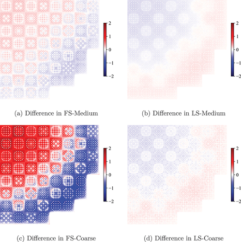
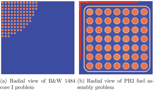
In this section, the LSA and LLSA are compared for the Babcock and Wilcox (B&W) 1484 core I benchmark problem^[48] and the Peach Bottom 2 (PB2) BWR single-assembly problem.^[49,50] The radial views of the problem geometries are shown in Fig. 14. Both problems are 3D; therefore, the 2D/1D method is used with the one-node P₃ nodal method for the axial direction. Both cases are divided into 40 planes in the axial direction. In this section, the LLSA is compared to the LSA for the coarse mesh and P₂ scattering source to look closely at the impact of LLSA.

Fig. 14. Problem geometries.

The simulation results for both cases are summarized in Tables XXIV and XXV. The LSA calculates negative sources in both problems. The negative LS does not occur at the beginning of the outer iterations in the B&W 1484 problem, but it occurs from the seventh outer iteration to the end of the iteration. The negative LS is calculated in 10 cells out of 40 490 cells. In the case of the PB2 problem, the negative LS is observed from the second outer iteration to convergence and is calculated in 1260 cells out of 62 069 cells.

TABLE XXIV Numerical Results from B&W 1484 Core I Simulations

Method	$\mathrm{\Delta }$$k_{\mathit{eff}}$ (pcm)	Maximum Difference in Pin Power (%)	Relative MOC Run Time	Relative Memory	Number of Cells with Negative LS^a
LSA	Reference	Reference	1.00	1.00	10
LLSA	$<$1	$<$0.01	1.05	1.00	0

^aThe total number of cells is 40 490.

TABLE XXV Numerical Results from PB2 Assembly Simulations

Method	$\mathrm{\Delta }$$k_{\mathit{eff}}$ (pcm)	Maximum Difference in Pin Power (%)	Relative MOC Run Time	Relative Memory	Number of Cells with Negative LS^a
LSA/split $\bar{q}+\bar{L}$	Reference	Reference	1.00	1.00	1260
LSA/split $\bar{L}$	$<$1	0.54	1.00	1.00	1260
LLSA	$<$1	0.06	1.06	1.00	0

^aThe total number of cells is 62 069.

For the PB2 assembly problem, an additional method (i.e., LSA/split $\mathit{L}$) was tested to determine the error caused by splitting TL only (i.e., ${\bar{L}}_{\mathit{i}}^{\mathit{g}}$) instead of the total source (i.e., ${\bar{q}}_{\mathit{i}}^{\mathit{g}}+{\bar{L}}_{\mathit{i}}^{\mathit{g}}$). In Sec. II.B.2, splitting ${\bar{L}}_{\mathit{i}}^{\mathit{g}}$ solely is discussed as an alternative method instead of using the LLSA. This method may reduce some parts of the negative LS. However, the method causes a considerable error due to the isotropic flux approximation. The maximum difference in the relative pin power distribution is 0.54% with this method. Moreover, the negative LS issue is not completely resolved. Fortunately, the negative LS does not lead to instability in either problem, but the possibility remains.

On the other hand, the LLSA does not calculate the negative LS in either case. There are minimal differences between the results from the LSA and LLSA. The maximum difference in the pin power distribution is 0.06%. This is because the LLSA changes the LS coefficient and splits the TL by as little as possible to maintain a nonnegative LS at the same time. It is concluded that the LLSA successfully resolves the negative LS issues caused by the LSA. There is a 5% to 6% run-time overhead from the LLSA compared to LSA. Most of the additional run time is used to find the minimum LS in Eq. (40)(40) ${\bar{q}}_{\mathit{i}}^{\mathit{g},min}=\underset{\mathit{m},\mathit{k}}{min}\left\{{\bar{q}}_{\mathit{aki}}^{\mathit{g}}\pm {\hat{q}}_{\mathit{mi}}^{\mathit{g}}\frac{{\mathit{t}}_{\mathit{mki}}}{2}\right\}.$(40) . The memory overhead is negligible.

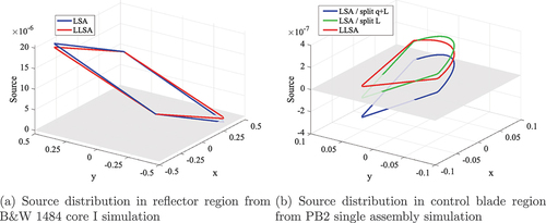
The source distribution is plotted in Fig. 15 to illustrate the difference between the LSA and LLSA. Figure 15a shows the LS at the reflector mesh. In the figure, $\mathit{x}$ and $\mathit{y}$ indicate the relative position from the center of the mesh. Figure 15a also shows that the LSA has some negative sources while the LLSA source is positive at all positions. The TL splitting was not performed for the B&W problem since the scattering and fission source are sufficiently large to compensate for the TL. Therefore, the difference between the LSA and the LLSA in Fig. 15a is solely caused by the gradient reduction of LS. The LLSA successfully prevents the negative LS by reducing the gradient—in strictly 2D problems.

Fig. 15. Comparisons between LSA and LLSA.

Consequently, refining the spatial mesh is a workaround to prevent the negative LS instead of using LLSA in 2D problems. The LSA with a smaller mesh may represent a more realistic source shape as it is. Specifically, the simulation with the LSA and refined coolant mesh (8×8 mesh per coolant pin) does not calculate the negative LS even though the result is not presented in this paper. However, this workaround has limitations since it needs a smaller mesh and there is no way to know how small of a mesh is needed before running it. Moreover, this workaround is only valid for a 2D case or 3D case that does not need TL splitting. If TL splitting is needed, half of the cell always has negative LS regardless of the mesh size. Therefore, it is necessary to use LLSA for robust 2D/1D simulations.

Figure 15b shows the source distributions at the end of the control blade mesh in the PB2 assembly problem. In contrast to the B&W problem, the TL splitting was performed for the PB2 problem. This may be because the PB2 problem has a more complicated configuration in the axial direction. As discussed in Sec. II.B.2, the LSA (i.e., LSA/split $\mathrm{q}$+$\mathrm{L}$ in Fig. 15b) has negative sources when the TL splitting is performed. This is clearly observed for the LSA in Fig. 15b. The average source is 0, and half of the mesh has a negative LS. The LSA with splitting TL only (i.e., LSA/split $\mathrm{L}$ in Fig. 15b) has a less negative LS; however, there is still some remaining negativity in the LS due to its steep gradient. This is why the negative LS was observed in Table XXV. On the other hand, the LLSA has positive sources in all cells. This example shows why the LLSA is necessary to adjust the quantity of the split source and the gradient of LS simultaneously to avoid the negative LS that may cause instability.

IV. DISCUSSION

In Sec. III, it is demonstrated that the LS-Coarse mesh is about 5% slower than that of FS-Medium mesh in the case of TCP₀ scattering. However, the LS-Coarse mesh is actually faster than FS-Medium in terms of overall run time thanks to the smaller number of mesh regions. In actual calculations, the subgroup MOC fixed source calculation is performed to calculate fuel (or resonance material) escape probabilities for the resonance self-shielding. In this calculation, the neutron source is represented with the intermediate resonance approximation with an assumed flat source over the mesh. Since the source is flat and fixed, it is not necessary to have a good spatial representation (such as a linear source) for the resonance self-shielding calculation. In general, the same mesh is used in the self-shielding calculation and the eigenvalue transport calculation.

Therefore, the subgroup MOC fixed source calculation with coarse mesh is very efficient with the coarse mesh without a significant loss of accuracy. Specifically, the coarse mesh option normally uses 50% fewer MOC segments than the medium mesh as presented in Sec. III. The run time of the subgroup MOC fixed source calculation is simply proportional to the number of MOC segments since only a flat source is used. Therefore, the LS-Coarse mesh has an about 2 times faster run time for the subgroup calculation than the FS-Medium mesh.

Overall, the LS-Coarse mesh is about 10% faster than the FS-Medium mesh in MPACT even for the TCP₀ scattering case, thanks to the run-time reduction in the subgroup calculation. This fact is not discussed in Sec. III to focus on the calculation performance of the MOC transport calculation. Additional run-time improvements may also be achieved in the depletion and TH feedback calculations thanks to the use of fewer regions.

The numerical results shown in Sec. III.F verified that the LLSA can eliminate the negative source, which may degrade convergence stability. The LLSA can be applied to the improved LSA described in this paper as well as the moment-based LSA in CASMO5.^[9] In MPACT, the LLSA method has been implemented and is used optionally if necessary. Although the negative LS is obviously harmful to the convergence, the negative LS rarely makes the iteration diverge. The LLSA has a 5% to 6% run-time overhead, which is not considered significant. At this time, how the emergence of a negative MOC source affects the convergence is still not well understood. This may be an area of future work. However, if a simulation is diverged due to a negative source, a user may try to use the LLSA method to resolve the issue. Otherwise, the method may be used conditionally.

V. CONCLUSIONS

This paper describes an improved LSA for the MOC to support efficient and robust multiphysics and 2D/1D applications. Ferrer and Rhodes developed the moment-based LSA and demonstrated the performance of the method against 2D and single-physics (i.e., neutronics) transport simulations.^[9] The moment-based LSA in Ref. [9] relies on precomputed coefficients with a cross-section dependence. The cross-section dependence of these coefficients leads to inefficiency in calculations where cross sections are not constant throughout, such as in multiphysics and 2D/1D applications.

A reformulation of this method is introduced that eliminates the cross-section dependence of these coefficients, without additional operations, allowing for more efficient calculations, using the LS MOC method. The reformulation may use less memory than the previous formulation since it is not necessary to use the precomputed coefficients that are functions of source regions and energy groups. Furthermore, a more numerically robust formulation of the LSA (i.e., LLSA) is introduced to eliminate the emergence of negative sources calculated during the LS MOC calculation. The LS MOC solver may calculate a negative source, which generally degrades numerical stability of convergence, due to steep a gradient of the linear source, or the TL splitting used in the 2D/1D method. The LLSA introduces a gradient reduction factor and a new source splitting method to prevent the negative source with minimal computational burden.

The newly developed method is implemented in MPACT, and the performance is demonstrated through several LWR problems. The objective of using the LS MOC method is to allow for use of a coarser mesh while maintaining accuracy, leading to lower overall run time. This work has demonstrated that a coarser mesh can be used even in cases with isotopic depletion and TH feedback. From the numerical results, it was verified that LS MOC with coarse mesh can improve the accuracy and computational performance compared to FS MOC with finer mesh. For the C5G7 benchmark, LS MOC with coarse mesh reduced the run time by 40% and memory by 15% with 1.5 times more accurate pin power results. For LWR assembly and core problems, LS MOC with coarse mesh calculated up to 2 times more accurate pin powers with less than 10% run-time overhead and reduced the memory by 10% to 20% in the case of TCP₀ scattering. The improvement was more dramatic in the case of P₂ scattering: LS MOC with a coarse mesh reduced the run time by 30% and memory by 40% while still improving the pin power accuracy by a factor of 1.5 to 2 times. It is also demonstrated that the LLSA successfully eliminates the negative LS that arises with the LSA.

Disclosure Statement

No potential conflict of interest was reported by the author(s).

Additional information

Funding

This material is based upon work supported under an Integrated University Program Graduate Fellowship. This research was partially supported by the Consortium for Advanced Simulation of Light Water Reactors www.casl.gov, and Energy Innovation Hub (http://www.energy.gov/hubs) for Modeling and Simulation of Nuclear Reactors under U.S. Department of Energy contract number DE-AC05-00OR22725.We would like to thank Constellation for initiating this project with Oak Ridge National Laboratory, Idaho National Laboratory, the University of Michigan, North Carolina State University, and the University of Illinois Urbana-Champaign under U.S. Department of Energy contract number DE-AC05-00OR22725. This research made use of the resources of the High Performance Computing Center at Idaho National Laboratory, which is supported by the Office of Nuclear Energy of the U.S. Department of Energy and the Nuclear Science User Facilities under contract number DE-AC07-05ID14517.

References

- J. R. ASKEW, “A Characteristics Formulation of the Neutron Transport Equation in Complicated Geometries,” AEEW-M–1108. United Kingdom Atomic Energy Authority (1972).
- MPACT TEAM, “MPACT Theory Manual, Version 2.2.0,” ORNL/TM-2016/476, Consortium for Advanced Simulation of Light Water Reactors (2016).
- B. KOCHUNAS et al., “VERA Core Simulator Methodology for Pressurized Water Reactor Cycle Depletion,” Nucl. Sci. Eng., 185, 1, 217 (2017); https://doi.org/10.13182/NSE16-39.
- P. T. PETKOV and T. TAKEDA, “Transport Calculations of MOX and UO2 Pin Cells by the Method of Characteristics,” J. Nucl. Sci. Technol., 35, 12, 874 (1998); https://doi.org/10.1080/18811248.1998.9733960.
- S. SANTANDREA, R. SANCHEZ, and P. MOSCA, “A Linear Surface Characteristics Approximation for Neutron Transport in Unstructured Meshes,” Nucl. Sci. Eng., 160, 1, 23 (2008); https://doi.org/10.13182/NSE07-69.
- C. TANG and S. ZHANG, “Development and Verification of an MOC Code Employing Assembly Modular Ray Tracing and Efficient Acceleration Techniques,” Ann. Nucl. Energy, 36, 8, 1013 (2009); https://doi.org/10.1016/j.anucene.2009.06.007.
- C. RABITI et al., “Quasi Linear Representation of the Isotropic Scattering Source for the Method of Characteristics,” Proc. Int. Conf. Mathematics, Computational Methods and Reactor Physics (M&C 2009), Saratoga Springs, New York, May 3–7, 2009, p. 461, American Nuclear Society (2009).
- A. HÉBERT, “High-Order Linear Discontinuous and Diamond Differencing Schemes Along Cyclic Characteristics,” Nucl. Sci. Eng., 184, 4, 591 (2016); https://doi.org/10.13182/NSE16-82.
- R. M. FERRER and J. D. RHODES, “A Linear Source Approximation Scheme for the Method of Characteristics,” Nucl. Sci. Eng., 182, 2, 151 (2016); https://doi.org/10.13182/NSE15-6.
- G. A. GUNOW, “Full Core 3D Neutron Transport Simulation Using the Method of Characteristics with Linear Sources,” PhD Thesis, Massachusetts Institute of Technology (2018).
- M. J. HALSALL, “Neutron Transport in WIMS by the Characteristics Method,” Trans. Am. Nucl. Soc., 68 (1993).
- P. PETKOV, T. TAKEDA, and T. MORI, “Comparison of the Flat and Linear Source Variants of the Method of Characteristics,” Ann. Nucl. Energy, 26, 10, 935 (1999); https://doi.org/10.1016/S0306-4549(98)00109-1.
- S. SANTANDREA and R. SANCHEZ, “Positive Linear and Nonlinear Surface Characteristic Schemes for the Neutron Transport Equation in Unstructured Geometries,” Proc. Int. Conf. Physics of Reactors (PHYSOR-2002), Seoul, Korea, October 7–10, 2002.
- R. LE TELLIER and A. HÉBERT, “On the Integration Scheme Along a Trajectory for the Characteristics Method,” Ann. Nucl. Energy, 33, 14–15, 1260 (2006); https://doi.org/10.1016/j.anucene.2006.07.010.
- E. MASIELLO, R. CLEMENTE, and S. SANTANDREA, “High Order Method of Characteristics for 2-D Unstructured Meshes,” Proc. Int. Conf. Mathematics, Computational Methods and Reactor Physics (M&C 2009), Saratoga Springs, New York, May 3–7, 2009, p. 3360, American Nuclear Society (2009).
- X. M. CHAI, K. WANG, and D. YAO, “The Linear Source Approximation in Three Dimension Characteristics Method,” Proc. Int. Conf. Mathematics, Computational Methods and Reactor Physics (M&C 2009), Saratoga Springs, New York, May 3–7, 2009, p. 474, American Nuclear Society ( 2009).
- K. S. SMITH, “Full-Core, 2-D, LWR Core Calculations with CASMO-4E,” Proc. Int. Conf. Physics of Reactors (PHYSOR-2002), Seoul, Korea, October 7–10, 2002.
- J. CHOE and D. LEE, “Development of Angle-Dependent Linear Source Approximation for Three-Dimensional Method of Characteristics Transport Analysis Method in STREAM,” Ann. Nucl. Energy, 181, 109572 (2023); https://doi.org/10.1016/j.anucene.2022.109572.
- B. COLLINS et al., “Stability and Accuracy of 3D Neutron Transport Simulations Using the 2D/1D Method in MPACT,” J. Comput. Phys., 326, 612 (2016); https://doi.org/10.1016/j.jcp.2016.08.022.
- K. D. LATHROP, “Spatial Differencing of the Transport Equation: Positivity vs. Accuracy,” J. Comput. Phys., 4, 4, 475 (1969); https://doi.org/10.1016/0021-9991(69)90015-1.
- Z. DODSON, B. KOCHUNAS, and E. LARSEN, “The Stability of Linear Diffusion Acceleration Relative to CMFD,” J. Nucl. Eng., 2, 4, 336 (2021); https://doi.org/10.3390/jne2040027.
- A. FITZGERALD, B. KOCHUNAS, and T. DOWNAR, “Improved Formulation of the Method of Characteristics with Linear Source for 2D/1D and Multiphysics Calculations,” Proc. Int. Conf. Mathematics and Computational Methods Applied to Nuclear Science and Engineering (M&C 2019). Portland, Oregon, August 25–29, 2019, American Nuclear Society (2019).
- N. F. HERRING et al., “Improved Anisotropic Linear Source Formulation for Multiphysics Problems,” Proc. PHYSOR 2020: Transition to a Scalable Nuclear Future, 2020, EPJ Web Conf., 247, 03003 (2021).
- S. CHOI and B. KOCHUNAS, “The Limited Linear Source Approximation of the Method of Characteristics for Mitigating Negative Sources,” Proc. Int. Conf. Mathematics Computational Methods Applied to Nuclear Science and Engineering (M&C 2021), Virtual Meeting, October 3–7, 2021, American Nuclear Society (2021).
- A. FITZGERALD, “Parallel 3-D Method of Characteristics with Linear Source and Advanced Transverse Integration,” PhD Thesis, University of Michigan (2020).
- A. HÉBERT, Applied Reactor Physics, Presses inter Polytechnique (2009).
- A. YAMAMOTO, Y. KITAMURA, and Y. YAMANE, “Computational Efficiencies of Approximated Exponential Functions for Transport Calculations of the Characteristics Method,” Ann. Nucl. Energy, 31, 9, 1027 (2004); https://doi.org/10.1016/j.anucene.2004.01.003.
- B. M. KOCHUNAS, “A Hybrid Parallel Algorithm for the 3-D Method of Characteristics Solution of the Boltzmann Transport Equation on High Performance Compute Clusters,” PhD Thesis, University of Michigan (2013).
- G. W. STEWART, Afternotes on Numerical Analysis, SIAM (1996).
- A. FITZGERALD and B. KOCHUNAS, “Fast Exponential Function Approximations for the Method of Characteristics with Linear Source,” Trans. Am. Nucl. Soc., 119, 645 (2018).
- S. SANTANDREA et al., “A Neutron Transport Characteristics Method for 3D Axially Extruded Geometries Coupled with a Fine Group Self-Shielding Environment,” Nucl. Sci. Eng., 186, 3, 239 (2017); https://doi.org/10.1080/00295639.2016.1273634.
- M. TABUCHI et al., “Convergence Analysis of MOC Inner Iterations with Large Negative Self-Scattering Cross-Section,” J. Nucl. Sci. Technol., 50, 5, 493 (2013); https://doi.org/10.1080/00223131.2013.785271.
- Y. S. JUNG, C. H. LEE, and M. A. SMITH, “Verification of High-Fidelity Neutronics Code PROTEUS for C5G7 Benchmark Problems,” Trans. Am. Nucl. Soc., 116, 1042 (2017).
- S. CHOI and D. LEE, “Three-Dimensional Method of Characteristics/Diamond-Difference Transport Analysis Method in STREAM for Whole-Core Neutron Transport Calculation,” Comput. Phys. Commun., 260, 107332 (2021); https://doi.org/10.1016/j.cpc.2020.107332.
- M. HURSIN, “Full Core, Heterogeneous, Time Dependent Neutron Transport Calculations with the 3D Code DeCART,” PhD Thesis, University of California, Berkeley (2010).
- B. W. KELLEY and E. W. LARSEN, “A Consistent 2D/1D Approximation to the 3D Neutron Transport Equation,” Nucl. Eng. Des., 295, 598 (Dec. 2015); https://doi.org/10.1016/J.NUCENGDES.2015.07.026.
- M. JARRETT et al., “Improved Accuracy in the 2-D/1-D Method with Anisotropic Transverse Leakage and Cross-Section Homogenization,” Nucl. Sci. Eng., 192, 3, 219 (2018); https://doi.org/10.1080/00295639.2018.1507186.
- Y. LIU et al., “Validation of Pin-Resolved Reaction Rates, Kinetics Parameters, and Linear Source MOC in MPACT,” Nucl. Sci. Eng., 195, 1, 50 (Aug. 2020); https://doi.org/10.1080/00295639.2020.1780853.
- K. SMITH and B. FORGET, “Challenges in the Development of High-Fidelity LWR Core Neutronics Tools,” Proc. Int. Conf. Mathematics and Computational Methods Applied to Nuclear Science and Engineering (M&C 2013), Sun Valley, Idaho, May 5–9, 2013, p. 1809, American Nuclear Society (2013).
- M. A. SMITH, E. E. LEWIS, and N. BYUNG CHAN, “Benchmark on Deterministic 2-D MOX Fuel Assembly Transport Calculations Without Spatial Homogenization,” Prog. Nucl. Energy, 48, 5, 383 (2006); https://doi.org/10.1016/j.pnucene.2006.01.002.
- A. ZHU et al., “An Optimally Diffusive Coarse Mesh Finite Difference Method to Accelerate Neutron Transport Calculations,” Ann. Nucl. Energy, 95, 116 (2016); https://doi.org/10.1016/j.anucene.2016.05.004.
- A. T. GODFREY, “VERA Core Physics Benchmark Progression Problem Specifications,” CASL-U-2012-0131-004, Rev. 4, Consortium for Advanced Simulation of Light Water Reactors (2014); https://corephysics.com/docs/CASL-U-2012-0131-004.pdf.
- C. LAWING, S. PALMTAG, and M. ASGARI, “BWR Progression Problems,” ORNL/TM-2020/1792. Oak Ridge National Laboratory (2021).
- K. SEOG KIM et al., “Development of the CASL-VERA V4.2m5 MPACT 51-Group Libraries with ENDF/B-VII. 0 and VII. 1,” Proc. Int. Conf. Mathematics and Computational Methods Applied to Nuclear Science and Engineering, Jeju, Korea, April 16–20, 2017, p. 16 (2017).
- A. YAMAMOTO et al., “Non-Equidistant Ray Tracing for the Method of Characteristics,” Proc. Int. Topl. Mtg. M&C 2005, Avignon, France, September 12–15, 2005.
- R. SALKO et al., “CTF: A Modernized, Production-Level, Thermal Hydraulic Solver for the Solution of Industry-Relevant Challenge Problems in Pressurized Water Reactors,” Nucl. Eng. Des., 397, 111927 (2022); https://doi.org/10.1016/j.nucengdes.2022.111927.
- E. WALKER et al., “Effects of Fuel Temperature-Shaping Functions on Xenon Oscillations,” Proc. Int. Conf. Physics of Reactors: Transition to a Scalable Nuclear Future (PHYSOR2020), Cambridge, United Kingdom, March 29–April 2, 2020, EPJ Web Conf., 247, 02025 (2020).
- M. N. BALDWIN et al., “Critical Experiments Supporting Close Proximity Water Storage of Power Reactor Fuel,” Technical Progress Report, July 1, 1978–September 30, 1978, Babcock and Wilcox Company (1978).
- N. H. LARSEN, “Core Design and Operating Data for Cycles 1 and 2 of Peach Bottom 2,” General Electric Company, Nuclear Energy Engineering Division (1978).
- J. SOLIS et al., “Boiling Water Reactor Turbine Trip (TT) Benchmark. Volume I: Final Specifications,” Organisation for Economic Co-operation and Development (2001).