A Precision Benchmark Suite for Nuclear Reactor Point Kinetics Equations via Converged Accelerated Taylor Series (CATS)

Abstract

Extreme benchmarks of 10 or more places for the point kinetics equations for time-dependent nuclear reactor power transients are rare. Therefore, to establish an extreme benchmark, we employ a Taylor series (TS) with continuous analytical continuation to solve the ordinary differential equations of point kinetics including feedback. Nonlinear Wynn-epsilon convergence acceleration confirms the highly precise solutions for neutron and precursor densities. Through adaptive partitioning of time intervals, the proposed Converged Accelerated Taylor Series, or CATS algorithm in double precision, automatically performs successive mesh refinement to obtain high-precision initial conditions for each subinterval, with the intent to reduce propagation error. Confirmation of 10 to 12 places comes from comparison to the BEFD (Backward Euler Finite Difference) algorithm in quadruple precision also developed by the author. We report benchmark results for common cases found in the literature including step, ramp, zigzag, and sinusoidal prescribed reactivity insertions and insertions with nonlinear adiabatic Doppler feedback. We also establish a suite of new prescribed reactivity insertions and insertions with feedback, based on reactivities with Taylor series representations as suggested by the CATS algorithm.

Keywords:

• Point kinetics
• convergence acceleration
• Taylor series
• adaptive partitioning
• numerical wrangling
• extreme benchmark precision

I. MOTIVATION

The numerical solution of the point kinetics equations (PKEs) characterizing nuclear reactor transients is one of the most noted computations in all of reactor physics. The PKEs admit few analytical solutions, so numerical means are necessary and consequently have drawn attention from nuclear engineers, applied mathematicians, and physicists. It is not surprising to find that nearly every well-known method of solving a system of ordinary differential equations (ODEs) has been applied to the PKEs. One only need survey the list of references found in this work and the references therein to verify the truth of this statement. Among the many proposed solutions have been Runge-Kutta (RK) methods of all orders including generalized RK^[1,2] and the Rosenbrock forms,^[3] exponential transform or basis functions,^[4] stiffness integrating factors,^[5] Padé approximants,^[6–8] Laplace transform inversion,^[9] piecewise constant reactivity approximations,^[10,11] finite difference and converged accelerated finite differences,^[12–14] and solutions of integral equations.^[15–17]

Such an important set of equations therefore demands adequate numerical standards of solution, or high-precision (often-called extreme) benchmarks, to ensure confidence in the many numerical algorithms that have been, or will be, proposed. A high-precision PKE benchmark, based on Taylor series (TS) called Converged Accelerated Taylor Series (CATS),^[18] appeared in the 2012 American Nuclear Society Mathematics and Computation Topical Meeting in Knoxville. However, although not in the mainstream, the CATS benchmark managed to contribute to the development of a considerable number of published algorithms since its first appearance. Along with a second benchmark based on Backward Euler Finite Difference (BEFD),^[19] the two algorithms are arguably the most precise found in today’s literature. My objective in this work therefore is to bring an updated and even more precise CATS version (at least to 10 places) to a wider audience and simultaneously to augment the existing examples of reactivity insertions with new and novel ones.

Our focus is to compute 10-place solutions to the PKEs from a fast, efficient, and straightforward TS expansion. PKEs find application in nuclear facilities worldwide as numerical simulators, where they are essential to the design and operation of next-generation reactors and research facilities. Aside from their practicality, there is a particular satisfaction associated with developing a reliable, efficient, straightforward, and competitive numerical solution for PKEs for a wide variety of transients. “Efficient and straightforward” are to be interpreted as “simple yet extraordinarily precise within a reasonable execution time.”

Taylor series solutions to the PKEs^[20–25] have been prominent and are arguably the most straightforward of all. Notably, the TS was one of the earliest solutions conceived of, but the approach never gained popularity as it was thought to have poor convergence. In addition, time step control is required, and the algorithm exhibits rather delicate numerical behavior because of its susceptibility to roundoff error. In his classical work, Vigil^[23] presented one of the most precise implementations of the TS solution through continuous analytical continuation (CAC). His work was truly ahead of its time. Vigil chose time steps to systematically reduce propagation and roundoff errors. The CAC concept still requires a time step since the TS representation is over a time interval. However, with reduced time steps, fewer terms in the series are necessary for convergence than otherwise, thus leading to a higher-precision evaluation in potentially less computational time. At long times, however, the algorithm still suffered from propagation error accumulation, as does any solution of an initial value problem, unless one takes precautions to reduce error propagation, as is done here.

Before addressing the numerical solution, it is natural to question the significance of a high-precision benchmark. It seems that five or six places would suffice, which indeed would be most practical. However, my aim is to go beyond practical and to push the boundaries of what is possible. Specifically, I address the question: Can a Taylor series serve as an extreme benchmark solution (9/10 places or better) for the PKEs? To further clarify, I have coined the term “extreme benchmark,” which I use for all benchmarks that I develop. The term refers to the number of places that one wants to achieve and depends on what one finds in the literature at the time of publication for the specific benchmark being developed. For PKEs, one finds in the literature mostly 6- or 7-place benchmarks, though because of my benchmarks, the number can be 10 or 11 places. So, here, to be conservative (though clearly we are 10 or better places), I have chosen the challenge of 9-or-better places as extreme to augment current literature.

The CATS algorithm implements the common TS approximation at the numerical margins of double precision (DP) arithmetic rather than with extended precision arithmetic to maintain computational simplicity and to be accessible. Thus, the term “extreme benchmark” means to find solutions to nine or more digits of precision by application of readily accessible DP arithmetic. We will explore the essential elements required to address extreme benchmarking including CAC, partitioning, adaptivity, convergence acceleration, numerical “wrangling” (to coin a word from cowboy culture), and benchmark confirmation.

We begin with the mathematical theory of the TS solution followed by the numerical formulation for high-precision. The first nine benchmarks considered in Tables 1 through 7 are those previously published in Ref. [18] but are now given to 11 or 12 places and checked against the BEFD benchmark. The next 15 are new to 10, 11, or 12 places. After an explanation of the CATS algorithm, the first (extreme) benchmark confirms the CATS algorithm for a step insertion demonstrating 23 places of precision in a quadruple precision (QP) calculation. The usual prescribed reactivity insertions found in the literature come next followed by nonlinear insertions including Doppler. The last two sections present a suite of new reactivity insertions including both nonlinear prescribed insertions and variations of nonlinear Doppler insertions.

II. MATHEMATICAL THEORY

We begin with the PKEs for an arbitrary number m of delayed neutron groups without an external source for simplicity:

(1a,b) $\begin{array}{rl}& \frac{\mathit{dN}\left(\mathit{t}\right)}{\mathit{dt}}=\left[\frac{\mathit{\rho }\left(\mathit{t},\mathit{N}\right)-\beta }{\mathrm{\Lambda }}\right]\mathit{N}\left(\mathit{t}\right)+\sum _{\mathit{i}=1}^m{\lambda }_i{C}_i\left(\mathit{t}\right)\\ & \frac{d{C}_i\left(\mathit{t}\right)}{\mathit{dt}}=\frac{{\mathit{\beta }}_i}{\mathrm{\Lambda }}\mathit{N}\left(\mathit{t}\right)-{\lambda }_i{C}_i\left(\mathit{t}\right),\mathit{\hspace{0.17em}}\mathit{i}=1,...,\mathit{m},\end{array}$(1a,b)

where N and C_i are the neutron and precursor densities; ρ is the reactivity, which may depend upon the neutron density and time t; β_i are the i’th delayed group yield directly from fission; β is the total yield from all groups; λ_i is the decay constant for the i’th delayed group; Λ = neutron generation time. All kinetic parameters except possibly reactivity are constant in time.

Next, we assume a time grid as shown in Fig. 1 for arbitrary time edits $\left\{t_0,t_1,...,t_j,...,t_J\right\}$, except $t_0\equiv 0$. Neutron and precursor densities at the time edits are the primary numerical objective. If expanded in a TS about the initial time t_j−1 of the edit interval $t_{\mathit{j}-1}\le \mathit{t}\le t_j$, the neutron, precursor densities, and reactivity, assumed to be piecewise infinitely differentiable within an interval, are

Fig. 1. Time edit grid.

(2a,b,c) $\left\{\begin{array}{c}{N}_j\left(\mathit{t}\right)\\ C_{\mathit{i},\mathit{j}}\left(\mathit{t}\right)\\ {\rho }_j\left(\mathit{t},N_j\right)-\mathit{\beta }\end{array}\right\}=\sum _{\mathit{n}=0}^{\mathrm{\infty }}\left\{\begin{array}{c}{N}_{\mathit{n},\mathit{j}-1}\\ C_{\mathit{i},\mathit{n},\mathit{j}-1}\\ {\rho }_{\mathit{n},\mathit{j}-1}-\mathit{\beta }{\delta }_{\mathit{n}0}\end{array}\right\}{\left(\mathit{t}-{\mathit{t}}_{\mathit{j}-1}\right)}^{\mathit{n}}.$(2a,b,c)

The notation for all TS coefficients is

(2d) $f_{\mathit{n},\mathit{j}}\equiv \frac{1}{\mathit{n}!}{\left.\frac{d^n\mathit{f}\left(\mathit{t}\right)}{\mathit{d}{t}^n}\right|}_{t_j}$(2d)

including a subscript j to indicate the time.

On multiplying TS as a Cauchy product,^[26] the first term on the right-hand side (RHS) of Eq. (1a)(1a,b) $\begin{array}{rl}& \frac{\mathit{dN}\left(\mathit{t}\right)}{\mathit{dt}}=\left[\frac{\mathit{\rho }\left(\mathit{t},\mathit{N}\right)-\beta }{\mathrm{\Lambda }}\right]\mathit{N}\left(\mathit{t}\right)+\sum _{\mathit{i}=1}^m{\lambda }_i{C}_i\left(\mathit{t}\right)\\ & \frac{d{C}_i\left(\mathit{t}\right)}{\mathit{dt}}=\frac{{\mathit{\beta }}_i}{\mathrm{\Lambda }}\mathit{N}\left(\mathit{t}\right)-{\lambda }_i{C}_i\left(\mathit{t}\right),\mathit{\hspace{0.17em}}\mathit{i}=1,...,\mathit{m},\end{array}$(1a,b) becomes

(2e) $\left[\frac{{\rho }_j\left(\mathit{t},N_j\right)-\mathit{\beta }}{\mathrm{\Lambda }}\right]N_j\left(\mathit{t}\right)=\frac{1}{\mathrm{\Lambda }}\sum _{\mathit{k}=0}^{\mathrm{\infty }}{\gamma }_{\mathit{k},\mathit{j}-1}{\left(\mathit{t}-{\mathit{t}}_{\mathit{j}-1}\right)}^{\mathit{k}},$(2e)

where

(2f) ${\gamma }_{\mathit{k},\mathit{j}}\equiv \sum _{\mathit{l}=0}^k\left({\rho }_{\mathit{k}-\mathit{l},\mathit{j}}-\mathit{\beta }{\delta }_{\mathit{k}-\mathit{l},0}\right)N_{\mathit{l},\mathit{j}}=\left({\rho }_{0,\mathit{j}}-\mathit{\beta }\right)N_{\mathit{k},\mathit{j}}+\sum _{\mathit{l}=0}^{\mathit{k}-1}{\rho }_{\mathit{k}-\mathit{l},\mathit{j}}{N}_{\mathit{l},\mathit{j}}.$(2f)

Substitution into the PKEs, with the RHS derivative appropriately represented as

(3) $\frac{d}{\mathit{dt}}\left\{\begin{array}{c}{N}_j\left(\mathit{t}\right)\\ C_{\mathit{i},\mathit{j}}\left(\mathit{t}\right)\end{array}\right\}=\sum _{\mathit{n}=0}^{\mathrm{\infty }}\mathit{n}\left\{\begin{array}{c}{N}_{\mathit{n},\mathit{j}-1}\\ C_{\mathit{i},\mathit{n},\mathit{j}-1}\end{array}\right\}{\left(\mathit{t}-{\mathit{t}}_{\mathit{j}-1}\right)}^{\mathit{n}-1},$(3)

gives the recurrences for the TS coefficients for $\mathit{n}=0,1,...$:

(4a,b) $\begin{array}{rl}& \left(\mathit{n}+1\right)N_{\mathit{n}+1,\mathit{j}}=\frac{1}{\mathrm{\Lambda }}{\gamma }_{\mathit{n},\mathit{j}}+\sum _{\mathit{i}=0}^m{\lambda }_i{C}_{\mathit{i},\mathit{n},\mathit{j}}\\ & \left(\mathit{n}+1\right)C_{\mathit{i},\mathit{n}+1,\mathit{j}}=\frac{{\beta }_i}{\mathrm{\Lambda }}{N}_{\mathit{n},\mathit{j}}-{\lambda }_i{C}_{\mathit{i},\mathit{n},\mathit{j}}.\end{array}$(4a,b)

Starting from critical at t₀, the starting terms for the recurrence come from the initial conditions:

(4c,d) $N_{0,0}=N_0\left(0\right)C_{\mathit{i},0,0}=\frac{{\beta }_i}{{\lambda }_i\mathit{\Lambda }}{N}_{0,0}.$(4c,d)

From continuity of the initial edit t_j−1 of edit interval j, the zeroth term of the TS is the neutron or precursor density at the end of the previous time interval t_j–1:

(5a) $\begin{array}{rl}& N_{\mathit{j}-1}\left(t_{\mathit{j}-1}\right)=N_j\left(t_{\mathit{j}-1}\right)=\sum _{\mathit{n}=0}^{\mathrm{\infty }}{N}_{\mathit{n},\mathit{j}-1}{\left({\mathit{t}}_{\mathit{j}-1}-t_{\mathit{j}-1}\right)}^{\mathit{n}}\\ & =N_{0,\mathit{j}-1}& (5\mathrm{a})\end{array}$(5a)

(5b) $\begin{array}{rl}& C_{\mathit{i},\mathit{j}-1}\left(t_{\mathit{j}-1}\right)=C_{\mathit{i},\mathit{j}}\left(t_{\mathit{j}-1}\right)=\sum _{\mathit{n}=0}^{\mathrm{\infty }}{C}_{\mathit{i},\mathit{n},\mathit{j}-1}{\left({\mathit{t}}_{\mathit{j}-1}-t_{\mathit{j}-1}\right)}^{\mathit{n}}\\ & =C_{\mathit{i},0,\mathit{j}-1},& (5\mathrm{b})\end{array}$(5b)

which is the definition of CAC. A key feature of the CATS algorithm is that once one assumes the TS for reactivity either from its functional form or, say, from a Padé approximant, the recurrence is complete with all coefficients deriving from Eqs. (4a,b(4a,b) $\begin{array}{rl}& \left(\mathit{n}+1\right)N_{\mathit{n}+1,\mathit{j}}=\frac{1}{\mathrm{\Lambda }}{\gamma }_{\mathit{n},\mathit{j}}+\sum _{\mathit{i}=0}^m{\lambda }_i{C}_{\mathit{i},\mathit{n},\mathit{j}}\\ & \left(\mathit{n}+1\right)C_{\mathit{i},\mathit{n}+1,\mathit{j}}=\frac{{\beta }_i}{\mathrm{\Lambda }}{N}_{\mathit{n},\mathit{j}}-{\lambda }_i{C}_{\mathit{i},\mathit{n},\mathit{j}}.\end{array}$(4a,b) ). Equations (2)(2a,b,c) $\left\{\begin{array}{c}{N}_j\left(\mathit{t}\right)\\ C_{\mathit{i},\mathit{j}}\left(\mathit{t}\right)\\ {\rho }_j\left(\mathit{t},N_j\right)-\mathit{\beta }\end{array}\right\}=\sum _{\mathit{n}=0}^{\mathrm{\infty }}\left\{\begin{array}{c}{N}_{\mathit{n},\mathit{j}-1}\\ C_{\mathit{i},\mathit{n},\mathit{j}-1}\\ {\rho }_{\mathit{n},\mathit{j}-1}-\mathit{\beta }{\delta }_{\mathit{n}0}\end{array}\right\}{\left(\mathit{t}-{\mathit{t}}_{\mathit{j}-1}\right)}^{\mathit{n}}.$(2a,b,c) , (3(3) $\frac{d}{\mathit{dt}}\left\{\begin{array}{c}{N}_j\left(\mathit{t}\right)\\ C_{\mathit{i},\mathit{j}}\left(\mathit{t}\right)\end{array}\right\}=\sum _{\mathit{n}=0}^{\mathrm{\infty }}\mathit{n}\left\{\begin{array}{c}{N}_{\mathit{n},\mathit{j}-1}\\ C_{\mathit{i},\mathit{n},\mathit{j}-1}\end{array}\right\}{\left(\mathit{t}-{\mathit{t}}_{\mathit{j}-1}\right)}^{\mathit{n}-1},$(3) ), and (4(4a,b) $\begin{array}{rl}& \left(\mathit{n}+1\right)N_{\mathit{n}+1,\mathit{j}}=\frac{1}{\mathrm{\Lambda }}{\gamma }_{\mathit{n},\mathit{j}}+\sum _{\mathit{i}=0}^m{\lambda }_i{C}_{\mathit{i},\mathit{n},\mathit{j}}\\ & \left(\mathit{n}+1\right)C_{\mathit{i},\mathit{n}+1,\mathit{j}}=\frac{{\beta }_i}{\mathrm{\Lambda }}{N}_{\mathit{n},\mathit{j}}-{\lambda }_i{C}_{\mathit{i},\mathit{n},\mathit{j}}.\end{array}$(4a,b) ) therefore define CAC (connecting edit subintervals) to provide the basis for extraordinary precision.

Theoretically, Eqs. (2a,b)(2a,b,c) $\left\{\begin{array}{c}{N}_j\left(\mathit{t}\right)\\ C_{\mathit{i},\mathit{j}}\left(\mathit{t}\right)\\ {\rho }_j\left(\mathit{t},N_j\right)-\mathit{\beta }\end{array}\right\}=\sum _{\mathit{n}=0}^{\mathrm{\infty }}\left\{\begin{array}{c}{N}_{\mathit{n},\mathit{j}-1}\\ C_{\mathit{i},\mathit{n},\mathit{j}-1}\\ {\rho }_{\mathit{n},\mathit{j}-1}-\mathit{\beta }{\delta }_{\mathit{n}0}\end{array}\right\}{\left(\mathit{t}-{\mathit{t}}_{\mathit{j}-1}\right)}^{\mathit{n}}.$(2a,b,c) are the true analytical solution representations—though not in closed form. Most importantly with Doppler feedback, when the reactivity is expressed as a piecewise continuous TS of the neutron density, the recurrence for the TS coefficients for the neutron density [Eqs. (4b,c)(4a,b) $\begin{array}{rl}& \left(\mathit{n}+1\right)N_{\mathit{n}+1,\mathit{j}}=\frac{1}{\mathrm{\Lambda }}{\gamma }_{\mathit{n},\mathit{j}}+\sum _{\mathit{i}=0}^m{\lambda }_i{C}_{\mathit{i},\mathit{n},\mathit{j}}\\ & \left(\mathit{n}+1\right)C_{\mathit{i},\mathit{n}+1,\mathit{j}}=\frac{{\beta }_i}{\mathrm{\Lambda }}{N}_{\mathit{n},\mathit{j}}-{\lambda }_i{C}_{\mathit{i},\mathit{n},\mathit{j}}.\end{array}$(4a,b) ] naturally lags the RHS relative to the left-hand side. Thus, the RHS is always numerically available without approximation, and the TS solution in the limit of an infinite number of terms becomes exact. Note that the previous statement is true only for piecewise continuous reactivity, which is always satisfied within an interval.

From a purely numerical consideration, besides roundoff error, there are two primary sources of numerical error associated with the TS solution of the PKEs. The first is the evaluation of the TS itself, or the series truncation error, and is the local error. The TS evaluation requires convergence of its partial sums, which in the limit admit convergence acceleration. The second error comes from the propagation of the local error from one time interval to the next like in a finite difference approximation. From Eqs. (5)(5a) $\begin{array}{rl}& N_{\mathit{j}-1}\left(t_{\mathit{j}-1}\right)=N_j\left(t_{\mathit{j}-1}\right)=\sum _{\mathit{n}=0}^{\mathrm{\infty }}{N}_{\mathit{n},\mathit{j}-1}{\left({\mathit{t}}_{\mathit{j}-1}-t_{\mathit{j}-1}\right)}^{\mathit{n}}\\ & =N_{0,\mathit{j}-1}& (5\mathrm{a})\end{array}$(5a) , we observed that the solution propagates through CAC and is continuous at an interval endpoint and the adjacent interval initial point. Minimization of the local and propagation errors is the essence of the CATS implementation through grid refinement and acceleration as discussed and demonstrated next.

III. NUMERICAL IMPLEMENTATION

III.A. Continuous Analytical Continuation with Partitioning

As already mentioned, to achieve extraordinary precision, we base the TS solution for the neutron and precursor densities on CAC with grid refinement convergence. Note, however, that we are primarily interested in the neutron density. To do so, one evaluates the recurrence of Eqs. (4)(4a,b) $\begin{array}{rl}& \left(\mathit{n}+1\right)N_{\mathit{n}+1,\mathit{j}}=\frac{1}{\mathrm{\Lambda }}{\gamma }_{\mathit{n},\mathit{j}}+\sum _{\mathit{i}=0}^m{\lambda }_i{C}_{\mathit{i},\mathit{n},\mathit{j}}\\ & \left(\mathit{n}+1\right)C_{\mathit{i},\mathit{n}+1,\mathit{j}}=\frac{{\beta }_i}{\mathrm{\Lambda }}{N}_{\mathit{n},\mathit{j}}-{\lambda }_i{C}_{\mathit{i},\mathit{n},\mathit{j}}.\end{array}$(4a,b) on the arbitrary discrete set of time edits t_j forming the edit intervals or subintervals [t_j–1,t_j] of the (total) interval [0,t_J] as shown in Fig. 1. Since the first coefficient initiates the recurrence, all coefficients follow, therefore enabling construction of the TS of Eqs. (2)(2a,b,c) $\left\{\begin{array}{c}{N}_j\left(\mathit{t}\right)\\ C_{\mathit{i},\mathit{j}}\left(\mathit{t}\right)\\ {\rho }_j\left(\mathit{t},N_j\right)-\mathit{\beta }\end{array}\right\}=\sum _{\mathit{n}=0}^{\mathrm{\infty }}\left\{\begin{array}{c}{N}_{\mathit{n},\mathit{j}-1}\\ C_{\mathit{i},\mathit{n},\mathit{j}-1}\\ {\rho }_{\mathit{n},\mathit{j}-1}-\mathit{\beta }{\delta }_{\mathit{n}0}\end{array}\right\}{\left(\mathit{t}-{\mathit{t}}_{\mathit{j}-1}\right)}^{\mathit{n}}.$(2a,b,c) to converge, in principle, to any precision. The concept of CAC therefore continues the TS solution between subintervals by continuity through the last subinterval. Generally, the smaller the time step (subinterval) is, the more quickly the TS convergence since fewer terms are necessary to converge the partial sums. Thus, high-precision convergence in a realistic computational time requires time step management. Therefore, we introduce additional partitioned subintervals within edit intervals along with convergence acceleration of the approximate solution at each edit t_j (as explained below).

III.B. Operational Flowchart Explained

The CATS algorithm is organized around edit subintervals specified at input as shown in the flowchart of Fig. 2 and further clarified. The desired edit is the endpoint of the interval [t_j–1,t_j], which is determined in Loop (A). However, in general, a more refined interval is required for efficient TS convergence; thus, the subintervals are refined in Loop (B) through further subdivision by partition.

Fig. 2. CATS algorithm operational flowchart.

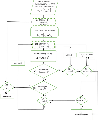
Refinement enables the TS (C) to converge more efficiently, either through acceleration or sequentially. Each refinement gives an approximate solution at the edit subinterval endpoint t_j and therefore together form a sequence of solutions for the densities. One monitors the sequence of densities to be either accelerated for convergence by the Wynn-epsilon (W-e) acceleration^[27] or allowed to naturally converge sequentially (G).

We now briefly outline the operational flow as shown in the flowchart of Fig. 2. The letters (A), (B), etc., in the diamond boxes refer to decisions with outcome y or n as indicated. The dashed outlined rectangles indicate the beginning of loops with their indices specified.

Referring to Fig. 2, the explanation of the algorithmic flow is as follows:

(A) Edit subinterval loop

Loop (A) specifies the j’th edit subinterval Δt_j = [t_j–1,t_j] to be partitioned eventually covering all J intervals over the total time interval [0,t_J].

(B) Partition of subinterval loop

The j’th edit interval is then sub-partitioned in Loop (B) according to^a

(6) $h_l=\frac{\mathrm{\Delta }{t}_j}{2^l}$(6)

for (partition) l in [l1,l2]^b to determine the densities at edit t_j for partition l.

(A/B/Cn/Dn/B) Convergence^c of TS?/Last l?

If the TS does not converge (Cn) at partition l within [l1,l2) of Loop (B) in (C), we discard the current partition l and increment l. Loop (B) partitioning continues unless l is the last l (l2), which is not yet true (Dn).

(A/B/Cn/Dy/En/B) Convergence of TS?/Last l?/Count ≤ 12?

If at the last l (Dy), the partition loop fails to give a converged TS for all densities at t_j, the original edit interval is partitioned by 2*ne, and the partition Loop (B) restarts for the newly formed partitions as long as the number (Count) of restarts is not greater than 12 (En).

(A/B/Cn/Dy/Ey/F) Convergence of TS?/Last l?/Count > 12?

If after 12 restarts of Loop (B), not all TS have converged at t_j (Ey), a manual restart (F, explained in IV.A) is called for, and the program stops. This means the TS in the partition loop did not all converge at edit t_j after dividing the edit subinterval into 2¹² subintervals. Further interval partitioning is therefore required.

(A/B/Cy/Gn/Hn/B) Convergence of TS?/Convergence of densities?/Last l?

If the TS has converged for some l in [l1,l2] of Loop (B), it is an approximation for the edit at t_j for the l’th partition. This adds to the sequence of solutions in l for which we also seek convergence. We then ask if the sequence at t_j has converged. If not (Gn), we check for the last l of the Loop (B). If not (Hn), l is incremented (ignoring the current l) as the (B) loop continues to build the sequence of solutions at t_j.

(A/B/Cy/Gn/Hy/Iny/B) Convergence of TS?/Convergence of densities and precursors?/Last l?/Count < > 12?

If at the last l (Hy) not exceeding 12 attempts (In), Loop (B) restarts with the original edit interval halved (Gn/Hy/In/B). After 12 restarts, a manual restart (Iy/F) is required, and the program stops.

(A/B/Cy/Gy/Jn/A) Convergence of TS?/Convergence of the densities and precursors?/Last j?

If all the TS have converged at some l (Cy) and the sequence of solutions for the densities has converged (Gy), we check for the last j. If true (Jy), we are done. If not (Jn), j is incremented, and the flow continues through Loops (A) and (B) until j is J.

III.C. Sequence Convergence

As noted in the algorithmic flowchart, there are two sequence convergences: one for the partial sums of the TS, say, for the neutron density at partition l,

(7a) $N_j\left(t_j;\mathit{l}\right)=\underset{\mathit{N}\to \mathrm{\infty }}{lim}\sum _{\mathit{n}=0}^N{N}_{\mathit{n},\mathit{j}-1}\left(\mathit{l}\right){\left(t_j-t_{\mathit{j}-1}\right)}^{\mathit{n}},$(7a)

and the second for the neutron density at edit t_j converging over the time steps defined by the partition l.

(7b) $N_j\left(t_j\right)=\underset{\mathit{l}\to \mathrm{\infty }}{lim}{N}_j\left(t_j;\mathit{l}\right).$(7b)

The means of convergence of Eqs. (7)(7a) $N_j\left(t_j;\mathit{l}\right)=\underset{\mathit{N}\to \mathrm{\infty }}{lim}\sum _{\mathit{n}=0}^N{N}_{\mathit{n},\mathit{j}-1}\left(\mathit{l}\right){\left(t_j-t_{\mathit{j}-1}\right)}^{\mathit{n}},$(7a) is convergence term-by-term, called natural or sequential convergence. In addition, we apply W-e convergence acceleration to extrapolate the sequences to their limits. W-e acceleration is a nonlinear acceleration assuming an extrapolated error series representation in terms of the sequence elements with unknown coefficients. A system of equations is constructed and solved with an extra equation for the approximation of the limit. In principle, the approximation should improve with the number of elements in the error series. Since the initial sequence elements are usually inaccurate, a window of elements for acceleration, nominally consisting of five elements, advances through the sequence list. Note that unlike Richardsons extrapolation,^[27] there is no regularity to the error series required for W-e making it virtually universal but possibly ineffective. We apply W-e acceleration to the sequences of TS partial sums of Eq. (7a)(7a) $N_j\left(t_j;\mathit{l}\right)=\underset{\mathit{N}\to \mathrm{\infty }}{lim}\sum _{\mathit{n}=0}^N{N}_{\mathit{n},\mathit{j}-1}\left(\mathit{l}\right){\left(t_j-t_{\mathit{j}-1}\right)}^{\mathit{n}},$(7a) and to the partitioned sequence solutions of Eq. (7b)(7b) $N_j\left(t_j\right)=\underset{\mathit{l}\to \mathrm{\infty }}{lim}{N}_j\left(t_j;\mathit{l}\right).$(7b) at each edit. Finally, the convergence mode, W-e or natural, whichever results in the least relative error between the last two sequence elements (called the “engineering” error estimate), becomes the sequence limit.

IV. NUMERICAL CONFIRMATION OF CATS ALGORITHM

To be clear, all tabular and graphical results to follow are for the neutron density normalized to one at time zero.

IV.A. Input Parameters and Convergence, Wrangling, and Agreement

To ensure a meaningful comparison, one compares the Double Precision Converged Accelerated Taylor Series (DPCATS) algorithm (called CATS) to the Quadruple Precision Backward Euler Finite Difference (QPBEFD) algorithm (called BEFD). This section describes how one compares the two benchmark solutions. In particular, on what basis is the comparison, and to what extent does CATS input adjustment play a role in providing a meaningful assessment.

Table A gives the nominal input parameter list (NIPL) with suggested values for the CATS algorithm. Parameter err is the relative error to determine convergence of the TS partial sums and the solution at each edit over the l-partitions. We define relative error as the difference between the last two sequence elements over the most recent element, which is an “engineering” estimate of Cauchy convergence. For example, if we expect 10 places, the relative error is set in the range of 10⁻¹² for DP arithmetic. A lower value could possibly incur roundoff error, though we will see several examples converge with a lower err. To get tighter TS convergence, an increase in the parameter m1 forces the TS to converge to a tighter relative error (err/10^m1).

TABLE A Nominal Input Parameter List (NIPL) for CATS

Parameter	Suggested Value	Description
err	10^−12 to 10^−15	Desired range of relative error
ne	1	Further partition of edit intervals in Loop (B)
ne1	1	One time partition of original edit intervals
l1/l2	4/11,12	Initial/final partition in Loop (B) [l1$\le$l$\le$l2]
K	15	Maximum number of terms for TS convergence
m1	0 to 3	TS over convergence index OCI (err/10^m1)
n0	5	Number of sequence elements in W-e window

Parameters ne1 and ne further divide the edit intervals for additional time step reduction. Parameter ne1 partitions the original edit intervals into ne1 partitions,

(8) $\mathrm{\Delta }{t}_j\to \frac{\mathrm{\Delta }{t}_j}{\mathbf{ne1}},$(8)

but only once at the start of the calculation, thus further reducing the time step to enable TS convergence within K terms. In addition, ne1 values make up the plots. As noted in the flowchart (Fig. 2) for loop (B/C/D/E/B), if the TS has not converged at a given partition, say, l–1 in Loop (B), the next partition interval $h_l$ [Eq. (7)(7a) $N_j\left(t_j;\mathit{l}\right)=\underset{\mathit{N}\to \mathrm{\infty }}{lim}\sum _{\mathit{n}=0}^N{N}_{\mathit{n},\mathit{j}-1}\left(\mathit{l}\right){\left(t_j-t_{\mathit{j}-1}\right)}^{\mathit{n}},$(7a) ] is partitioned by a factor 2*ne

(9) $h_l\to h_l/(2\ast \mathit{ne})=\frac{1}{2\ast \mathbf{ne}}\frac{\mathrm{\Delta }{t}_j}{2^l},$(9)

and Loop (B) continues at l. With partition adjustment, the intervals can be made as small as necessary to give efficient TS convergence. In addition, partition adjustments allow numerical wrangling.

The value l1 (nominally 4) denotes where the Loop (B) partition begins, which is important for TS convergence. The larger l1 is, the smaller the time step and faster convergence is. Partition l2, which nominally can be either 11 or 12, ends the solution sequence for each edit. The larger l2 is, the more elements are in the sequence increasing the potential for convergence without further time step reduction, i.e., avoidance of loop (B/C/D/E/B) shown in Fig. 2, but requiring more CPU.

The number of terms for TS to converge is restricted to K for the neutron and precursor densities, which is nominally 15 in current comparisons. If not converged within K terms, the TS is declared failed and ignored, the partition advances to l + 1, and the calculation of Loop (B) continues. The same is true if convergence is to any negative density. Referring to the flowchart of Fig. 2, failure to converge to a positive value at or before partition l2 (En) forces further partitions [by factor 2*ne; see Eq. (9(9) $h_l\to h_l/(2\ast \mathit{ne})=\frac{1}{2\ast \mathbf{ne}}\frac{\mathrm{\Delta }{t}_j}{2^l},$(9) )], and Loop (B) continues. Any combination of TS failures can occur in [l1,l2] 12 times before a manual adjustment is necessary (Ey/F). One then proceeds by choosing from the following adjustments and restarting:

1. Increase the initial number of partitions (i.e., ne1) to reduce the time step in Loop (B) in order to induce TS convergence.

2. Increase l1 to further reduce the step or increase l2 to extend partitions to produce more sequence elements.

3. Increase K to ease the TS convergence limitation.

4. Reduce or increase the over convergence index (OCI) (i.e., m1) to converge the TS with higher precision. To be considered nominal, m1 is 0 to 3.

5. Increase the W-e window n0 to provide a better opportunity for W-e convergence. n0 should be no larger than 15.

6. Increase or decrease the desired relative error err.

Thus, selections of adjustments are available to enable TS convergence and numerical wrangling for potential full agreement with BEFD.

CATS solutions are not unique with regard to the choice of input parameters because of the considerable number of input parameters (seven) with each choice defining a different path to sequence convergence. Since extreme benchmarks live between the 9th and 12th digit, we are comparing solutions at the margin of DP computational precision, which practically is no more than 12 digits. Thus, the choice of the input parameter list (NIPL) has a significant impact on the last digit. Here is where wrangling comes in. Since we are in the unique position of knowing the 12-place benchmark from BEFD, one could simply adjust or wrangle the partitions through the NIPL to try to eventually match the known benchmark by trial and error. But, what value is such an exercise with regard to verification of the CATS algorithm since, except in this rare situation, we never have the true benchmark to compare to? The best outcome would be that on convergence, all 12 places match (within the NIPL ranges of l2, m1, and err) and CATS would be verified to 12 places. Chances of this occurring are small. Wrangling the NIPL therefore offers the possibility of verifying a number of places, say, 10, which we know to be true, thus providing a measure of precision of the CATS algorithm. The least amount of wrangling, the higher the confidence in the precision. If a benchmark like BEFD is unavailable, then wrangling is the same as a sensitivity study, which is common sense verification of a solution. The precision would then be how close two solutions are with respect to number of places when, say, err or m1 are varied. For the purpose of our investigation, however, we use wrangling in a controlled way to address our curiosity regarding exactly how close the two algorithms actually are. Thus, wrangling does play a role in CATS verification at several levels.

To limit excessive wrangling possibly leading nowhere and to provide some consistency, we suggest the following wrangling guidelines based on the application of the boldface values (NIPL) of Table A. If agreement is fewer than 10 or 11 places,

1. Change m1 from 0 to 3 with l2 = 11.

2. Still no agreement, increase l2 to 12 for better TS convergence and again try m1 from 0 to 3.

3. Still no agreement, reduce relative error err to 10⁻¹³, 10⁻¹⁴, or 10⁻¹⁵. Chances are convergence will be lost when err is too low however.

4. Still no agreement, set l2 to 14, 15, or 16 and m1 = 2 or 3.

5. Still no agreement, increase ne1 to 16 or ne to 16 or both for (c) or (d).

6. Set ne1 to 100 in (e).

For each benchmark, the outcome, with or without wrangling, is included as a table of BEFD results with an overlay of CATS results and the differences marked. In this way, the 12-place BEFD benchmark is available, and, simultaneously, the precision of CATS is evident. An accompanying narrative gives the details of the wrangling required. Two categories of wrangling exist: minor and major. Minor wrangling includes steps (a), (b), (c), and (d), which would naturally be part of a sensitivity study of any solution. Major wrangling includes steps (e) and (f), which are not obvious and require guessing and trial and error. Minor wrangling could conceivably be applied to all CATS benchmarks as a sensitivity study, but major wrangling is for a known benchmark thus requiring, in our case, BEFD. We record all input lists in Table B.I of Appendix B including computational time.

Several comments are in order. While 10-place agreement emerges most readily, 11 and 12 places may not. Here is where one wrangles just to see if higher agreement is indeed possible. However, noting that 10 places accomplishes our original extreme benchmark goal, we limit excessive wrangling usually to several discrepancies in the 12th place. The premise is that a 10-place CATS benchmark is sufficient since it is still high precision in the PKE literature, but if we can establish more places, all the better. Note, however, that regardless, we always publish the 12-place BEFD benchmark as the reference.

Since we are creating a benchmark for a given set of edits (usually from 5 to 10), the precision of any benchmark may depend upon the choice of edits because they determine the partitions. Therefore, there is a degree of uncontrolled uncertainty associated with establishing a high-precision benchmark, which is unavoidable. However, experience has shown that 10 places are relatively independent of variation of the choice of the NIPL and edits as will become obvious in the examples to follow.

Finally, a third independent comparison option is always available, and that is Quadruple Precision Converged Accelerated Taylor Series (QPCATS); however, CPU will be greatly increased. Nevertheless, QP is a last resort for verification, which we apply on three occasions in this investigation.

IV.B. An Extreme Benchmark Comparison

To show that the CATS algorithm indeed gives a reliable benchmark, we consider a step reactivity insertion of $0.5 in Fast Reactor I (FRI) in the extreme. Reactor kinetic parameters for all benchmarks in our study are in the tables of Appendix A with FRI Table A.I. The first appearance of this benchmark seems to be in Nobrega^[7] and ever since has served as a standard for comparison for newly developed numerical RKE algorithms. It is well known for step reactivities that there exists an analytical solution via diagonalization of the Jacobian matrix to solve the scalar ODEs on the diagonal coupled through eigenvectors. Since the analytical solution has appeared in texts (see Ref. [28], for example), we skip its derivation.

As mentioned, the existence of the BEFD algorithm^[19] puts us in a unique situation regarding comparisons. First published to precision better than one unit in the ninth place, the BEFD algorithm is a fundamental finite difference solution for all densities with iteration for nonlinear reactivity feedback. The BEFD algorithm also includes sequence convergence with acceleration on an adaptive mesh to mitigate propagation error. Recently, in a relatively thorough investigation, the BEFD algorithm was compared to the physics informed neural net (PINN) precise formulation X-TFC^[29] to, in some cases, 12 places. The PINN comparison gives confidence in the BEFD benchmark for what follows. However, to ensure a proper comparison, we execute BEFD in QP to be certain of at least 12 places of precision when compared to CATS in DP.

For all comparisons, the number of digits minus 1 in agreement (number of places), primarily for the neutron density at a given time edit, is the benchmarking measure. Each case includes a table of only the BEFD benchmark results for 10, 11, and 12 places, expected to be precise including the last digit quoted. The discrepant digits in comparison to CATS will be in boldface type in the table. An underscored digit, such as , indicates the CATS digit is below BEFD, and if underscored, such as X, CATS is above BEFD. In either case, the discrepancy is a single unit. If the digit is only highlighted, then the discrepancy is more than one unit either above or below BEFD.

Table 1a presents the results of an extreme precision example to 23 places for step reactivity insertion with both BEFD and CATS in QP and including the analytical solution in QP by diagonalization. This is the first of three instances of CATS executed in QP. One finds perfect agreement to all places for all three solutions, which gives additional confidence in the BEFD benchmark for the CATS comparisons to follow.

TABLE 1a Extreme Precision Demonstration: Step Insertion into FRI (ρ₀ = $0.5, Λ = 10⁻⁷s)

t(s)	QPBEFD/QPCATS/QPAnalytical
0.0000E+00	1.00000000000000000000000E+00
1.0000E−01	2.07531716248122033152682E+00
1.0000E+00	2.65585295935837676143711E+00
1.0000E+01	1.27465396678628924693564E+01
1.0000E+02	1.31287276940349626158236E+07

With BEFD established as a credible benchmark, at least for step insertions, in the following demonstrations, we compare DPCATS to QPBEFD (called CATS and BEFD, respectively) anticipating at least 10 or more place agreement. As will be shown, because of variability associated with the NIPL, in particular, partitioning, the 11th or 12th place can require numerical wrangling to achieve full agreement—especially for the 12th place. We now continue toward our goal of a minimum of 9 places of agreement for a common NIPL including only minor wrangling and possibly full agreement with major wrangling.

IV.C. Further Verification

Table 1b is a continuation of the initial demonstration for the NIPL of Table A to establish a 12-place benchmark. The number in parenthesis in the column headings indicates the number of precise digits in that column. Note that, while unnecessary, columns of 10, 11 and 12 digits are provided for each benchmark. This is to confirm all digits and to also, in some cases, justify rounding error. As observed, both benchmarks agree to all 12 digits (since no digits are boldface).

TABLE 1b Neutron Density Confirmation: Step Reactivity into FRI (ρ₀ = $0.5, Λ = 10⁻⁷s)

t(s)	(10)	(11)	(12)	Reference [7]	Convergence
0.0000E+00	1.0000000000E+00	1.00000000000E+00	1.000000000000E+00	1.000000E+00
1.0000E–01	2.0753171625E+00	2.07531716248E+00	2.075317162481E+00	2.075317E+00	1
1.0000E+00	2.6558529594E+00	2.65585295936E+00	2.655852959358E+00	2.655853E+00	1
1.0000E+01	1.2746539668E+01	1.27465396679E+01	1.274653966786E+01	1.274654E+01	2
1.0000E+02	1.3128727694E+07	1.31287276940E+07	1.312872769403E+07	—	2

Table 1c compares the precursor densities to 11 places. For the NIPL there is only one discrepancy in the 11th place in delayed group 2 at t = 10s. It seems that no amount of wrangling eliminates this discrepancy without causing discrepancies at other entries. However, QPCATS agrees with BEFD at 12 times the CPU of DPCATS and is the second instance where QP is used to show agreement.

TABLE 1c Precursor Density Confirmation: Step Reactivity into FRI (ρ₀ = $0.5, Λ = 10⁻⁷s)

t(s)/m	1	2	3	4	5	6
0.0000E+00	1.29612403101E+05	3.96141479100E+05	7.09253731343E+04	4.35951661631E+04	3.59841269841E+03	4.79750778816E+02
1.0000E−01	1.29785770834E+05	3.97417778603E+05	7.19049645570E+04	4.50681476487E+04	4.04075603004E+03	6.16699564464E+02
1.0000E+00	1.31839871541E+05	4.12418201067E+05	8.29098959659E+04	6.02777250697E+04	7.22324746594E+03	1.16488836072E+03
1.0000E+01	2.13283235626E+05	9.77487790540E+05	4.04343149675E+05	3.71865336497E+05	4.07151646027E+04	5.82683889600E+03
1.0000E+02	1.31850995210E+11	8.75792669859E+11	4.33872945342E+11	3.90947865256E+11	4.21097025638E+10	6.01091977254E+09

Figure 3 displays the decadal neutron density trace for a $0.5 step showing the initiation of the delayed neutron contribution at early time and the prompt neutrons at late time. Table 1d gives a decadal benchmark over 18 temporal decades as confirmed by BEFD to all 12 digits quoted. The primary mode of convergence is W-e acceleration as indicated by “2” in the last column. “1” is conventional sequential convergence.

Fig. 3. Decadal time variation of the density step reactivity into FRI.

TABLE 1d Decadal Variation: Step Reactivity into FRI (ρ₀ = $0.5, Λ = 10⁻⁷s)

t(s)	BEFD/CATS(10)	BEFD/CATS(11)	BEFD/CATS(12)	Convergence
1.0000E−15	1.0000000000E+00	1.00000000002E+00	1.000000000022E+00
1.0000E−14	1.0000000002E+00	1.00000000022E+00	1.000000000220E+00	2
1.0000E−13	1.0000000022E+00	1.00000000220E+00	1.000000002200E+00	1
1.0000E−12	1.0000000220E+00	1.00000002200E+00	1.000000022000E+00	2
1.0000E−11	1.0000002200E+00	1.00000022000E+00	1.000000220000E+00	2
1.0000E−10	1.0000022000E+00	1.00000220000E+00	1.000002199998E+00	2
1.0000E−09	1.0000219998E+00	1.00002199976E+00	1.000021999758E+00	1
1.0000E−08	1.0002199758E+00	1.00021997580E+00	1.000219975802E+00	2
1.0000E−07	1.0021975818E+00	1.00219758177E+00	1.002197581774E+00	2
1.0000E−06	1.0217597650E+00	1.02175976501E+00	1.021759765011E+00	2
1.0000E−05	1.1974812583E+00	1.19748125831E+00	1.197481258310E+00	2
1.0000E−04	1.8892203637E+00	1.88922036370E+00	1.889220363704E+00	1
1.0000E−03	2.0007068176E+00	2.00070681763E+00	2.000706817634E+00	1
1.0000E−02	2.0076811958E+00	2.00768119583E+00	2.007681195831E+00	1
1.0000E−01	2.0753171625E+00	2.07531716248E+00	2.075317162481E+00	1
1.0000E+00	2.6558529594E+00	2.65585295936E+00	2.655852959358E+00	2
1.0000E+01	1.2746539668E+01	1.27465396679E+01	1.274653966786E+01	2
1.0000E+02	1.3128727694E+07	1.31287276940E+07	1.312872769403E+07	2

With the benchmarking procedure now in place, we are ready to demonstrate the CATS high-precision benchmark on a variety of standard and new insertions.

V. SELECTED DEMONSTRATIONS OF PRESCRIBED REACTIVITY INSERTIONS

The following demonstrations are representative of cases found in the literature including standard prescribed reactivity insertions covering negative step, ramp, and sinusoidal. For all cases, a table of 10-, 11- and 12-place benchmarks is presented for the neutron density from the BEFD benchmark determined in QP to 14 or 15 places with CATS results overlaid (see Sec. IV.B for explanation).

V.A. Negative Step Insertions

We now consider Thermal Reactor I (TRI) with parameters from Table A.II of Appendix A for negative step insertions of –$0.5 and –$1. We see perfect agreement in Tables 2a,b between the two algorithms to 12 digits.

TABLES 2a,b Negative Step:−$0.5/−$1 Step Reactivities into TRI (Λ = 5×10⁻⁴s)

ρ	t(s)	BEFD/CATS(10)	BEFD/CATS(11)	BEFD/CATS(12)	Convergence
(a) −$0.5	0.0000E+00	1.0000000000E+00	1.00000000000E+00	1.000000000000E+00
	1.0000E−01	6.9892522557E−01	6.98925225571E−01	6.989252255707E−01	2
	1.0000E+00	6.0705356561E−01	6.07053565606E−01	6.070535656062E−01	2
	5.0000E+00	4.8255302992E−01	4.82553029922E−01	4.825530299222E−01	2
	1.0000E+01	3.9607769072E−01	3.96077690715E−01	3.960776907155E−01	2
	1.0000E+02	7.1582854439E−02	7.15828544386E−02	7.158285443859E−02	1
	2.0000E+02	1.6934791659E−02	1.69347916587E−02	1.693479165875E−02	2
(b) −$1.0	0.0000E+00	1.0000000000E+00	1.00000000000E+00	1.000000000000E+00
	1.0000E−01	5.2056428661E−01	5.20564286609E−01	5.205642866088E−01	2
	1.0000E+00	4.3333344530E−01	4.33333445301E−01	4.333334453006E−01	1
	5.0000E+00	3.1067776843E−01	3.10677768428E−01	3.106777684278E−01	1
	1.0000E+01	2.3611065079E−01	2.36110650789E−01	2.361106507888E−01	2
	1.0000E+02	2.8667642454E−02	2.86676424545E−02	2.866764245448E−02	2
	2.0000E+02	5.5905967933E−03	5.59059679335E−03	5.590596793349E−03	2

V.B. Ramp Insertions

We next consider ramp insertions of $0.1 and $1s⁻¹ in Thermal Reactor II, whose kinetic parameters are in Table A.III of Appendix A. The PKEs for a reactivity ramp insertion do not have an analytical solution and can reach large densities quickly as shown in Table 3a for the first ramp. Again, we find perfect agreement.

TABLE 3a Ramp Reactivity: $0.1s^–1 Ramp into TRII (Λ =5×10^–4s)

t(s)	BEFD/CATS(10)	BEFD/CATS(11)	BEFD/CATS(12)	Convergence
0.0000E+00	1.0000000000E+00	1.00000000000E+00	1.000000000000E+00
2.0000E+00	1.3382000500E+00	1.33820005005E+00	1.338200050049E+00	2
4.0000E+00	2.2284418968E+00	2.22844189681E+00	2.228441896810E+00	1
6.0000E+00	5.5820524487E+00	5.58205244867E+00	5.582052448674E+00	1
8.0000E+00	4.2786295731E+01	4.27862957311E+01	4.278629573112E+01	1
1.0000E+01	4.5116362391E+05	4.51163623909E+05	4.511636239090E+05	2
1.1000E+01	1.7922136073E+16	1.79221360734E+16	1.792213607343E+16	1

For the second ramp insertion of $1s⁻¹ into FRI with the comparison shown in Table 3b for the nominal case with err set to 8 × 10⁻¹⁵ and m1 set to 2, we see agreement for 10 and 11 places and one entry multiple units off for 12 places. Further, if we continue wrangling and let ne = ne1 = 16 and l1 = 2, which are not obvious changes, we get perfect agreement. Thus, minor wrangling is unnecessary for a 10- or 11-place benchmark, but to reproduce BEFD perfectly, major wrangling is necessary, which is a judgment call.

TABLE 3b Ramp Reactivity: $1s^–1 Ramp into FRI (Λ =5×10^–4s, err = 8×10⁻¹⁵)

t(s)	BEFD/CATS(11)	BEFD/CATS(11)	BEFD/CATS(12)	Convergence
0.0000E+00	1.0000000000E+00	1.00000000000E+00	1.000000000000E+00
1.0000E−02	1.0100971112E+00	1.01009711118E+00	1.010097111175E+00	2
1.0000E−01	1.1133201123E+00	1.11332011226E+00	1.113320112264E+00	2
2.0000E−01	1.2605599250E+00	1.26055992496E+00	1.260559924957E+00	2
5.0000E−01	2.1364091074E+00	2.13640910738E+00	2.136409107379E+00	2
1.0000E+00	1.2078141972E+03	1.20781419722E+03	1.207814197221E+03	1
1.1000E+00	3.2575933547E+99	3.25759335471E+99	3.257593354712E+99	2
1.1500E+00	1.0289753595+219	1.02897535952+219	1.028975359518+219	1

V.C. Zig-Zag Insertion

We now come to one of the more exotic insertions, the Zig-Zag insertion into TRI (Table A.II). The Zig-Zag insertion consist of four legs of up and down insertions as follows:

(10) $\mathit{\rho }\left(\mathit{t}\right)=\left\{\begin{array}{c}0.0075\mathit{t},\mathit{\hspace{0.17em}}0\le \mathit{t}\le 0.5\mathrm{s}\\ -0.0075\left(\mathit{t}-0.5\right)+0.00375,\mathit{\hspace{0.17em}}0.5\mathrm{s}\le \mathit{t}\le 1\mathrm{s}\\ 0.0075\left(\mathit{t}-1\right),\mathit{\hspace{0.17em}}1\mathrm{s}\le \mathit{t}\le 1.5\mathrm{s}\\ 0.00375,\mathit{\hspace{0.17em}}1.5\mathrm{s}\le \mathit{t}\end{array}\right.$(10)

giving a piecewise continuous insertion, but not piecewise smooth. For this reason, each leg is viewed as a separate insertion, so the TS solution is applied piecewise over the entire interval. As observed in Table 4, perfect agreement is achieved for the NIPL with m1 = 2. Also note the majority of edits converged by W-e acceleration.

TABLE 4 Zig-Zag Insertion into TRI (Λ = 5×10^–4s)

t(s)	BEFD/CATS(10)	BEFD/CATS(11)	BEFD/CATS(12)	Convergence
0.0000E−01	1.0000000000E+00	1.00000000000E+00	1.000000000000E+00
5.0000E−01	1.7214224221E+00	1.72142242208E+00	1.721422422085E+00	2
1.0000E+00	1.2111274148E+00	1.21112741483E+00	1.211127414825E+00	1
1.5000E+00	1.8922261404E+00	1.89222614039E+00	1.892226140394E+00	2
2.0000E+00	2.5216005300E+00	2.52160053000E+00	2.521600530004E+00	2
1.0000E+01	1.2047105355E+01	1.20471053548E+01	1.204710535483E+01	2
1.0000E+02	6.8155568885E+07	6.81555688848E+07	6.815556888477E+07	2

The Zig-Zag example shows that by segmenting reactivity, any set of piecewise continuous reactivity insertions is permissible.

V.D. Sinusoidal Insertions

Next, we consider one delayed group sinusoidal insertion into Fast Reactor II (FRII) with kinetic parameters

(11) $\begin{array}{rl}& \mathit{\beta }=0.0079\\ & \mathit{\lambda }=0.077{\mathrm{s}}^{-1}\\ & \mathrm{\Lambda }=1\times {10}^{-7}\mathrm{s}.\end{array}$(11)

For this fast transient, the reactivity varies as

(12a) $\mathit{\rho }\left(\mathit{t}\right)={\rho }_{0}sin\left(\mathit{\gamma t}\right).$(12a)

The TS coefficients are

(12b) ${\rho }_{\mathit{n},\mathit{j}}={\left(-1\right)}^{\left[\mathit{n}/2\right]}\frac{{\gamma }^n}{\mathit{n}!}{\rho }_0\left\{\begin{array}{c}sin\left(\mathit{\gamma }{t}_j\right),\mathit{n}\mathit{even}\\ cos\left(\mathit{\gamma }{t}_j\right),\mathit{n}\mathit{odd},\end{array}\right.$(12b)

or more conveniently,

(12c) ${\rho }_{\mathit{n},\mathit{j}}=\frac{{\gamma }^n}{\mathit{n}!}{\rho }_0\left[cos\left(\mathit{n\pi }/2\right)sin\left(\mathit{\gamma }{t}_j\right)+sin\left(\mathit{n\pi }/2\right)cos\left(\mathit{\gamma }{t}_j\right)\right],$(12c)

which simplifies to

(13) ${\rho }_{\mathit{n},\mathit{j}}=\frac{{\gamma }^n}{\mathit{n}!}{\rho }_{0}sin\left(\mathit{\gamma }{t}_j+\mathit{n\pi }/2\right),$(13)

where $\mathit{\gamma }\equiv \mathit{\pi }/50{\mathrm{s}}^{-1}$ and ${\rho }_0=\mathrm{\$}0.005333$.

Figure 4 is a plot of the neutron density variation, and the benchmark comparison is in Table 5a. With an OCI of m1 = 3, we find convergence to 10 and 11 places as well as 12 places for t < 10s. The CPU time for Table 5a was exceptionally long at 107s. Of course, this gives at least 11 places of precision, but if only 9 places were called for, the CPU would be 30s less.

Fig. 4. Neutron density for one delayed group sinusoidal reactivity insertion into FRII.

TABLE 5a One Delayed Group Sinusoidal Reactivity Insertion into FRII (ρ₀ = $0.005333, γ = π/50s⁻¹, Λ = 10⁻⁷s)

t(s)	BEFD/CATS(10)	BEFD/CATS(11)	BEFD/CATS(12)	Convergence
0.0000E+00	1.0000000000E+00	1.00000000000E+00	1.000000000000E+00
1.0000E−02	1.0004239597E+00	1.00042395973E+00	1.000423959732E+00	1
1.0000E−01	1.0042754809E+00	1.00427548091E+00	1.004275480913E+00	2
1.0000E+00	1.0460190642E+00	1.04601906418E+00	1.046019064184E+00	1
1.0000E+01	2.0652644823E+00	2.06526448228E+00	2.06526448227E+00	1
1.0000E+02	1.5440238789E+01	1.54402387889E+01	1.544023878889E+01	1

For the second sinusoidal variation, we consider a six delayed group TRI (Table A.II) version, where $\mathit{\gamma }\equiv \mathit{\pi }/150{\mathrm{s}}^{-1}$ and ${\rho }_0=\mathrm{\$}0.003233$ with results shown in Table 5b. One observes 12-place precision, when l1 = 5 and m1 = 1, but for several units in the last entry.

TABLE 5b Six Delayed Group Sinusoidal Reactivity Insertion into TRI (ρ₀ = $0.003233, γ = π/150s⁻¹)

t(s)	BEFD/CATS(10)	BEFD/CATS(11)	BEFD/CATS(12)	Convergence
0.0000E+00	1.0000000000E+00	1.00000000000E+00	1.000000000000E+00
1.0000E−02	1.0000064453E+00	1.00000644531E+00	1.000006445312E+00	2
1.0000E−01	1.0004374069E+00	1.00043740686E+00	1.000437406860E+00	1
1.0000E+00	1.0096671690E+00	1.00966716902E+00	1.009667169017E+00	2
1.0000E+01	1.2039760355E+00	1.20397603551E+00	1.203976035506E+00	2
1.0000E+02	3.2103073547E+03	3.21030735465E+03	3.210307354653E+03	2

VI. SELECTED DEMONSTRATIONS OF NONLINEAR ADIABATIC DOPPLER AND DENSITY-DEPENDENT INSERTIONS

We now are concerned with non-linear adiabatic Doppler feedback reactivity of the form

(14a) $\mathit{\rho }\left(\mathit{t}\right)={\rho }_0\left(\mathit{t}\right)-\mathit{B}\underset{0}{\overset{t}{\int }}\mathit{dt}{ }^{\mathrm{\prime }}\mathit{N}\left(\mathit{t}{ }^{\mathrm{\prime }}\right),$(14a)

where ${\rho }_0\left(\mathit{t}\right)$ is prescribed and B is the given temperature coefficient of reactivity. The second term is the Doppler integral term adding negative reactivity proportional to reactor heating. By taking the n’th derivative

(14b) $\frac{d^n}{\mathit{d}{t}^n}\underset{0}{\overset{t}{\int }}\mathit{dt}{ }^{\mathrm{\prime }}\mathit{N}\left(\mathit{t}{ }^{\mathrm{\prime }}\right)=\frac{{\mathit{d}}^{\mathit{n}-1}}{\mathit{d}{t}^{\mathit{n}-1}}\frac{d}{\mathit{dt}}\underset{0}{\overset{t}{\int }}\mathit{dt}{ }^{\mathrm{\prime }}\mathit{N}\left(\mathit{t}{ }^{\mathrm{\prime }}\right)=N^{\left(\mathit{n}-1\right)}\left(\mathit{t}\right),$(14b)

the n’th TS coefficient of reactivity at edit t_j is simply

(15) ${\rho }_{\mathit{n},\mathit{j}}={\rho }_{0,\mathit{n},\mathit{j}}-\frac{B}{n}{N}_{\mathit{n}-1,\mathit{j}}.$(15)

VI.A. Step Insertion with Doppler

For a step insertion ${\rho }_0$, we have for $N_{-1,\mathit{j}}\equiv 0$, the following TS coefficient:

(16) ${\rho }_{\mathit{n},\mathit{j}}={\rho }_0{\delta }_{\mathit{n},0}-\frac{B}{k}{N}_{\mathit{n}-1,\mathit{j}}.$(16)

Now, consider the kinetics parameters of Thermal Reactor IV in Table A.V with Λ = 5×10⁻⁵s and B = 2.5×10⁻⁶/MWs. Figure 5 shows how the Doppler feedback effectively stops transients of step reactivity insertions of $0.1 to $2. Tables 6a,b,c give neutron densities for insertions of $1, $1.5, and $2, respectively. For the $1 insertion with m1 = 1, we observe one discrepancy in the 12th digit by a single unit. When err is 10⁻¹⁴, the discrepancy vanishes however. For the $1.5 insertion with the same NIPL, there are no discrepancies for m1 set to 2 and l2 set to 12, respectively. We see perfect agreement for the $2 insertion when m1 is 2.

Fig. 5. Neutron density for adiabatic feedback and six step insertions.

TABLES 6a,b,c Neutron Densities for Insertions of $1, $1.5, and $2.

(a) ρ0 = $1, Λ = 5x10^−5s
t(s)	BEFD/CATS(10)	BEFD/CATS(11)	BEFD/CATS(12)	conv
0.0000E+00	1.0000000000E+00	1.00000000000E+00	1.000000000000E+00
1.0000E+00	8.0527812545E+02	8.05278125449E+02	8.052781254488E+02	2
1.0000E+01	1.3194585878E+02	1.31945858778E+02	1.319458587776E+02	2
2.0000E+01	5.1675599140E+01	5.16755991398E+01	5.167559913980E+01	2
3.0000E+01	2.8165478123E+01	2.81654781231E+01	2.816547812308E+01	2
4.0000E+01	1.8141812575E+01	1.81418125753E+01	1.814181257533E+01	2
5.0000E+01	1.2776961432E+01	1.27769614317E+01	1.277696143166E+01	2
6.0000E+01	9.4732419528E+00	9.47324195281E+00	9.473241952811E+00	2
7.0000E+01	7.2433002064E+00	7.24330020643E+00	7.243300206432E+00	2
8.0000E+01	5.6454283755E+00	5.64542837546E+00	5.645428375455E+00	2
9.0000E+01	4.4561837084E+00	4.45618370844E+00	4.456183708438E+00	2
1.0000E+02	3.5496012141E+00	3.54960121408E+00	3.549601214084E+00	2
(b) ρ0 = $1.5, Λ = 5x10^−5s
0.0000E+00	1.0000000000E+00	1.00000000000E+00	1.000000000000E+00
1.0000E+00	8.1094972780E+02	8.10949727799E+02	8.109497277989E+02	1
1.0000E+01	1.0787694512E+02	1.07876945123E+02	1.078769451229E+02	1
2.0000E+01	4.1596896088E+01	4.15968960884E+01	4.15968960883E+01	2
3.0000E+01	2.3296227711E+01	2.32962277105E+01	2.329622771050E+01	2
4.0000E+01	1.5302087318E+01	1.53020873175E+01	1.530208731751E+01	2
5.0000E+01	1.0889353812E+01	1.08893538118E+01	1.088935381184E+01	2
6.0000E+01	8.1005133978E+00	8.10051339775E+00	8.100513397754E+00	1
7.0000E+01	6.1823251167E+00	6.18232511674E+00	6.182325116740E+00	1
8.0000E+01	4.7930388494E+00	4.79303884942E+00	4.793038849418E+00	1
9.0000E+01	3.7554112321E+00	3.75541123207E+00	3.755411232072E+00	2
1.0000E+02	2.9659185490E+00	2.96591854900E+00	2.965918548995E+00	2
(c) ρ0 = $2, Λ = 5x10^−5s
0.0000E+00	1.0000000000E+00	1.00000000000E+00	1.000000000000E+00
1.0000E+00	8.1329909944E+02	8.13299099435E+02	8.132990994355E+02	2
1.0000E+01	1.0335691805E+02	1.03356918046E+02	1.033569180456E+02	2
2.0000E+01	3.9134327846E+01	3.91343278459E+01	3.913432784591E+01	1
3.0000E+01	2.2002158526E+01	2.20021585264E+01	2.200215852640E+01	2
4.0000E+01	1.4492870628E+01	1.44928706275E+01	1.449287062751E+01	2
5.0000E+01	1.0318137565E+01	1.03181375650E+01	1.031813756503E+01	2
6.0000E+01	7.6630069808E+00	7.66300698080E+00	7.663006980800E+00	1
7.0000E+01	5.8291748686E+00	5.82917486862E+00	5.829174868621E+00	2
8.0000E+01	4.4992647619E+00	4.49926476188E+00	4.499264761876E+00	2
9.0000E+01	3.5073002243E+00	3.50730022434E+00	3.507300224338E+00	1
1.0000E+02	2.7550331306E+00	2.75503313062E+00	2.755033130619E+00	1

It is comforting that the NIPL gives perfect agreement between the benchmarks with only minor adjustments.

VI.B. Keepin’s Compensated Ramp Insertion

We next consider Keepin’s compensated ramp insertion^[9] with adiabatic Doppler feedback

(17) $\begin{array}{rl}& {\rho }_{0,\mathit{j}}=0\\ & {\rho }_{1,\mathit{j}}=\mathit{a}\\ & {\rho }_{\mathit{n},\mathit{j}}=-\frac{B}{n}{N}_{\mathit{n}-1,\mathit{j}},\mathit{\hspace{0.17em}}\mathit{n}=2,3,& (17)\end{array}$(17)

and proceed as previously for four ramp rates a and two Doppler coefficients B.

Figure 6 shows the Doppler effect again effectively shutting down the transient after a short but increasing time with decreasing ramp rate initiating the transient. The figure is virtually identical to that of the classic work of Keepin.^[9] Tables 7a–h present a comparison between CATS and BEFD neutron densities for the eight transients. For the NIPL with m1 = 0, all 11 places agree with only 6 entries for all tables disagreeing in the 12th place (not shown). For m1 = 2, all discrepancies vanish except for the second-to-last entry of case h (boldface), which vanishes if err is set to 5 × 10⁻¹³ as found by minor wrangling.

Fig. 6. Compensated ramp insertion as in Keepin.^[9]

One should note that more than 70% of the edits (51/72) converge by convergence acceleration in 0.67s of CPU time. If we suppress acceleration, the computational time reduces to 0.14s but with three discrepancies. In comparison, if we only allow acceleration, the CPU time is 7s with one discrepancy. Curiously, all three calculations with acceleration, with no acceleration, and for the choice of acceleration or no acceleration have the same discrepant entry in Table 7h. Including acceleration does increase computational time but, nevertheless, enables the choice of either natural or accelerated convergence, which seems to have a time advantage over acceleration only (i.e., 0.67s vs 7s). Most importantly, including acceleration increases confidence in the computation as it provides an additional verification.

TABLES 7a–h Neutron Densities for Ramps into TRIII with Doppler

(a) a = 0.1s^−1 B = 10^−11/MWs
t(s)	BEFD/CATS(10)	BEFD/CATS(11)	BEFD/CATS(12)	conv
0.0000E+00	1.0000000000E+00	1.00000000000E+00	1.000000000000E+00
1.0000E−01	2.4733658212E+01	2.47336582123E+01	2.473365821230E+01	2
5.0000E−01	9.9498932412E+09	9.94989324117E+09	9.949893241175E+09	2
1.0000E+00	1.0104242001E+10	1.01042420007E+10	1.010424200070E+10	2
2.0000E+00	1.0068310736E+10	1.00683107364E+10	1.006831073642E+10	2
3.0000E+00	1.0049143594E+10	1.00491435935E+10	1.004914359353E+10	2
4.0000E+00	1.0037600560E+10	1.00376005596E+10	1.003760055960E+10	2
5.0000E+00	1.0029740467E+10	1.00297404665E+10	1.002974046651E+10	1
7.5000E+00	1.0017984257E+10	1.00179842572E+10	1.001798425721E+10	2
1.0000E+01	1.0011886158E+10	1.00118861582E+10	1.001188615822E+10	2
(b) a = 0.0s^−1 B = 10^−11/MWs
0.0000E+00	1.0000000000E+00	1.00000000000E+00	1.000000000000E+00
1.0000E−01	1.1672108377E+00	1.16721083771E+00	1.167210837715E+00	1
5.0000E−01	4.2699528441E+00	4.26995284405E+00	4.269952844053E+00	2
1.0000E+00	1.4823509385E+07	1.48235093847E+07	1.482350938467E+07	2
2.0000E+00	1.0016052907E+09	1.00160529072E+09	1.001605290724E+09	2
3.0000E+00	1.0617721285E+09	1.06177212854E+09	1.061772128536E+09	2
4.0000E+00	1.0442587702E+09	1.04425877016E+09	1.044258770157E+09	2
5.0000E+00	1.0337982900E+09	1.03379829001E+09	1.033798290011E+09	2
7.5000E+00	1.0194902855E+09	1.01949028546E+09	1.019490285462E+09	2
1.0000E+01	1.0124316714E+09	1.01243167142E+09	1.012431671425E+09	2
(c) a = 0.003s^−1 B = 10^−11/MWs
0.0000E+00	1.0000000000E+00	1.00000000000E+00	1.000000000000E+00
1.0000E−01	1.0453716663E+00	1.04537166630E+00	1.045371666299E+00	1
5.0000E−01	1.3246619846E+00	1.32466198459E+00	1.324661984585E+00	2
1.0000E+00	2.0531949811E+00	2.05319498114E+00	2.053194981136E+00	1
2.0000E+00	2.3920639689E+01	2.39206396888E+01	2.392063968876E+01	2
3.0000E+00	8.0570978433E+08	8.05709784331E+08	8.057097843307E+08	1
4.0000E+00	3.4133407009E+08	3.41334070087E+08	3.413340700868E+08	1
5.0000E+00	3.2932662695E+08	3.29326626954E+08	3.293266269537E+08	2
7.5000E+00	3.2271921821E+08	3.22719218212E+08	3.227192182120E+08	1
1.0000E+01	3.1459364163E+08	3.14593641634E+08	3.145936416341E+08	1
(d) a = 0.001s^−1 B = 10^−11/MWs
0.0000E+00	1.0000000000E+00	1.00000000000E+00	1.000000000000E+00
1.0000E−01	1.0147177710E+00	1.01471777105E+00	1.014717771047E+00	2
5.0000E−01	1.0898213935E+00	1.08982139354E+00	1.089821393537E+00	2
1.0000E+00	1.2136025788E+00	1.21360257879E+00	1.213602578792E+00	1
2.0000E+00	1.6144148814E+00	1.61441488145E+00	1.614414881449E+00	1
3.0000E+00	2.4471103261E+00	2.44711032608E+00	2.447110326079E+00	2
4.0000E+00	4.6439263602E+00	4.64392636023E+00	4.643926360228E+00	2
5.0000E+00	1.4163711393E+01	1.41637113932E+01	1.416371139317E+01
7.5000E+00	1.2592678382E+09	1.25926783818E+09	1.259267838179E+09	2
1.0000E+01	1.5900586024E+08	1.59005860241E+08	1.590058602409E+08	2
(e) a = 0.1s^−1 B = 10^−13/MWs
0.0000E+00	1.0000000000E+00	1.00000000000E+00	1.000000000000E+00
1.0000E−01	2.4733658251E+01	2.47336582509E+01	2.473365825088E+01	2
5.0000E−01	1.5433617863E+12	1.54336178629E+12	1.543361786285E+12	2
1.0000E+00	1.0100735783E+12	1.01007357828E+12	1.010073578280E+12	2
2.0000E+00	1.0068324164E+12	1.00683241638E+12	1.006832416382E+12	2
3.0000E+00	1.0049146603E+12	1.00491466032E+12	1.004914660322E+12	1
4.0000E+00	1.0037601614E+12	1.00376016137E+12	1.003760161371E+12	2
5.0000E+00	1.0029740921E+12	1.00297409214E+12	1.002974092136E+12	2
7.5000E+00	1.0017984372E+12	1.00179843719E+12	1.001798437192E+12	1
1.0000E+01	1.0011886207E+12	1.00118862073E+12	1.001188620726E+12	2
(f) a = 0.01s^−1 B = 10^−13/MWs
0.0000E+00	1.0000000000E+00	1.00000000000E+00	1.000000000000E+00
1.0000E−01	1.1672108379E+00	1.16721083792E+00	1.167210837918E+00	1
5.0000E−01	4.2699528644E+00	4.26995286440E+00	4.269952864400E+00	2
1.0000E+00	1.4833155106E+07	1.48331551059E+07	1.483315510587E+07	2
2.0000E+00	9.2815225125E+10	9.28152251255E+10	9.281522512546E+10	2
3.0000E+00	1.0620282033E+11	1.06202820331E+11	1.062028203309E+11	2
4.0000E+00	1.0446043780E+11	1.04460437803E+11	1.044604378025E+11	2
5.0000E+00	1.0338896655E+11	1.03388966548E+11	1.033889665484E+11	2
7.5000E+00	1.0194999125E+11	1.01949991252E+11	1.019499912524E+11	2
1.0000E+01	1.0124348832E+11	1.01243488316E+11	1.012434883158E+11	2
(g) a = 0.003s^−1 B = 10^−13/MWs
0.0000E+00	1.0000000000E+00	1.00000000000E+00	1.000000000000E+00
1.0000E−01	1.0453716665E+00	1.04537166646E+00	1.045371666458E+00	1
5.0000E−01	1.3246619862E+00	1.32466198617E+00	1.324661986171E+00	2
1.0000E+00	2.0531949903E+00	2.05319499029E+00	2.053194990288E+00	1
2.0000E+00	2.3920642249E+01	2.39206422487E+01	2.392064224873E+01	1
3.0000E+00	6.3125860906E+11	6.31258609057E+11	6.312586090572E+11	2
4.0000E+00	3.3555955479E+10	3.35559554785E+10	3.355595547852E+10	1
5.0000E+00	3.2156761131E+10	3.21567611308E+10	3.215676113084E+10	2
7.5000E+00	3.2102051821E+10	3.21020518214E+10	3.210205182144E+10	2
1.0000E+01	3.1456146867E+10	3.14561468668E+10	3.145614686684E+10	1
(h) a = 0.001s^−1 B = 10^−13/MWs
0.0000E+00	1.0000000000E+00	1.00000000000E+00	1.000000000000E+00
1.0000E−01	1.0147177712E+00	1.01471777120E+00	1.014717771195E+00	2
5.0000E−01	1.0898213945E+00	1.08982139454E+00	1.089821394541E+00	2
1.0000E+00	1.2136025816E+00	1.21360258156E+00	1.213602581557E+00	2
2.0000E+00	1.6144148929E+00	1.61441489293E+00	1.614414892934E+00	1
3.0000E+00	2.4471103706E+00	2.44711037061E+00	2.447110370609E+00	2
4.0000E+00	4.6439265876E+00	4.64392658765E+00	4.643926587648E+00	2
5.0000E+00	1.4163713862E+01	1.41637138620E+01	1.416371386202E+01	1
7.5000E+00	8.3616177063E+09	8.36161770625E+09	8.361617706254E+09	2
1.0000E+01	1.6158767668E+10	1.61587676681E+10	1.615876766808E+10	2

VI.C. Insertion Proportional to Neutron Density

A more straightforward nonlinear density-dependent feedback is proportionality to the neutron density itself

(18a) $\mathit{\rho }\left(\mathit{t}\right)=0.1\mathit{\beta N}\left(\mathit{t}\right),$(18a)

to give the TS coefficients

(18b) ${\rho }_{\mathit{n},\mathit{j}}=0.1\mathit{\beta }{N}_{\mathit{n},\mathit{j}},\mathit{\hspace{0.17em}}\mathit{n}=0,1,....$(18b)

We choose Thermal Reactor II of Table A.IV with neutron lifetime of 5 × 10⁻⁴s. Table 8a confirms that all entries but two (off by one unit) are in perfect agreement to 12 places (for m1 set to 2). The last two digits come into compliance when the err is set to 5 × 10⁻¹⁵.

TABLE 8a Proportional Insertion TRII (Λ = 5×10⁻⁴s, err = 10⁻¹²)

t(s)	BEFD/CATS(10)	BEFD/CATS(11)	BEFD/CATS(12)	Convergence
0.0000E+00	1.0000000000E+00	1.00000000000E+00	1.000000000000E+00
1.0000E−01	1.0817840726E+00	1.08178407260E+00	1.081784072596E+00	2
5.0000E−01	1.1435623844E+00	1.14356238440E+00	1.143562384399E+00	2
1.0000E+00	1.1676688085E+00	1.16766880850E+00	1.167668808496E+00	2
2.0000E+00	1.2079218113E+00	1.20792181132E+00	1.207921811316E+00	2
5.0000E+00	1.3199424643E+00	1.31994246426E+00	1.319942464258E+00	1
1.0000E+01	1.5296094953E+00	1.52960949528E+00	1.529609495280E+00	2
1.5000E+01	1.8179563592E+00	1.81795635915E+00	1.817956359151E+00	1
2.0000E+01	2.3139472813E+00	2.31394728130E+00	2.313947281298E+00	2
2.5000E+01	4.0904249107E+00	4.09042491066E+00	4.09042491066E+00	2
2.6000E+01	9.1631391167E+00	9.16313911667E+00	9.16313911667E+00	1

This insertion is particularly interesting since the neutron density becomes unbounded in a finite time. Figure 7 shows the steep ascent with time at about 26s. As time approaches 26.163683⁺s, the neutron density approaches infinity. Apparently, the neutron density becomes infinite in the interval [26.163683588, 26.163683589], which needs further verification.

Fig. 7. Neutron density approach to infinity.

The sudden change in agreement between DPCATS and BEFD in the second column of Table 8b indicates that higher-precision arithmetic is required to track the neutron density as it approaches infinity. This is evident when QPCATS (third application of QP) is included in column 3 and is observed to match BEFD to 10 places. When we evaluate at times closer to the singularity as shown in Table 8c, QPCATS responds with larger and larger numbers, but BEFD fails to converge (not shown). We conclude that CATS can do this exceptional case but only with QP arithmetic.

TABLE 8b Asymptotic Approach of Neutron Density to Infinity (Λ = 2×10^–5s, err = 8×10⁻¹⁵)

t(s)	DPCATS(10)	QPCATS(10)	BEFD(10)
2.6000000E+01	9.1631391167E+00	9.1631391167E+00	9.1631391167E+00
2.6100000E+01	1.6795369146E+01	1.6795369146E+01	1.6795369146E+01
2.6160000E+01	2.1373243263E+02	2.1373243263E+02	2.1373243263E+02
2.6163000E+01	1.1299299378E+03	1.1299299378E+03	1.1299299378E+03
2.6163600E+01	9.2047441902E+03	9.2047441929E+03	9.2047441929E+03
2.6163630E+01	1.4354947695E+04	1.4354947701E+04	1.4354947701E+04
2.6163683E+01	1.3064063145E+06	1.3064063682E+06	1.3064063682E+06

TABLE 8c Approach to Singularity

t(s)	QPCATS(10)
26.163683000000	1.3064063682E+06
26.163683588000	1.2101591483E+09
26.163683588568	1.1401156760E+10

VII. ADDITIONAL PRESCRIBED REACTIVITY INSERTIONS

During the past 50 years, few if any new reactivity insertions have appeared in the literature as benchmarks. That is about to change as we investigate several new prescribed reactivities as suggested by the CATS algorithm and confirmed by the BEFD algorithm. Since CATS requires reactivity in the form of a power series (TS) to be input into the recurrence of Eq. (4a)(4a,b) $\begin{array}{rl}& \left(\mathit{n}+1\right)N_{\mathit{n}+1,\mathit{j}}=\frac{1}{\mathrm{\Lambda }}{\gamma }_{\mathit{n},\mathit{j}}+\sum _{\mathit{i}=0}^m{\lambda }_i{C}_{\mathit{i},\mathit{n},\mathit{j}}\\ & \left(\mathit{n}+1\right)C_{\mathit{i},\mathit{n}+1,\mathit{j}}=\frac{{\beta }_i}{\mathrm{\Lambda }}{N}_{\mathit{n},\mathit{j}}-{\lambda }_i{C}_{\mathit{i},\mathit{n},\mathit{j}}.\end{array}$(4a,b) , virtually any common function is a suitable reactivity candidate making the possibilities practically limitless. In essence, only the n’th TS coefficient ${\rho }_{\mathit{n},\mathit{j}}$ of the reactivity is necessary. In this regard, we review several ways of generating TS. Since BEFD only requires the reactivity as a given function, we can simultaneously confirm the CATS benchmark and in so doing establish a suite of new PKE benchmarks. Aside from including Doppler, the reactivities considered do not necessarily represent physical transients and are to be viewed simply as benchmarks.

Our approach is to choose the four example reactivities inserted into TRIII, shown in Table B, and determine their TS coefficients using one of four methods: differentiation, McLaurin series, recurrence, and from literature. From these examples, we then construct additional reactivities in the following section.

TABLE B Example Reactivity Insertions

Insertion	ρ(t)	ρ0	α	μ	σ	γ
Exponential	${\rho }_0{e}^{-\mathit{\alpha t}}$	$1	0.25, 0.5, 1s^–^1	—	—	—
Sine	${\rho }_{0}sin\left(\mathit{\gamma t}\right)$	$1	—	—	—	0.3, 0.6, 0.8s^–^1
Shifted Gaussian	$\frac{{\rho }_0}{\sqrt{2\mathit{\pi }}\mathit{\sigma }}{e}^{-{\left(\mathit{t}-\mathit{\mu }\right)}^2/2{\sigma }^2}$	$1	—	0.1, 1, 3, 10, 20s	0.5, 1, 2, 3s	—
Bessel function	${\rho }_0{J}_0\left(\mathit{\alpha t}\right)$	$0.2, 0.4, 0.6, 0.8, 1	0.5, 1, 5s^–^1	—	—	—

VII.A. Selected Reactivity Insertions into TRIII

VII.A.1. Exponential Insertion: By Differentiation

Consider an exponential insertion

(19) $\mathit{\rho }\left(\mathit{t}\right)={\rho }_0{e}^{-\mathit{\alpha t}},t_{\mathit{j}-1}\le \mathit{t}\le t_j.$(19)

The most straightforward way to find the Taylor coefficients for reactivity is simply differentiate n times to give the TS coefficient at t_j–1:

(20) ${\rho }_{\mathit{n},\mathit{j}-1}={\rho }_0\frac{{\left(-1\right)}^n}{\mathit{n}!}{\alpha }^n{e}^{-\mathit{\alpha }{\mathit{t}}_{\mathit{j}-1}},\mathit{\hspace{0.17em}}\mathit{n}=0,1,....$(20)

Incorporating the coefficient into the CATS algorithm through the recurrence of Eq. (4)(4a,b) $\begin{array}{rl}& \left(\mathit{n}+1\right)N_{\mathit{n}+1,\mathit{j}}=\frac{1}{\mathrm{\Lambda }}{\gamma }_{\mathit{n},\mathit{j}}+\sum _{\mathit{i}=0}^m{\lambda }_i{C}_{\mathit{i},\mathit{n},\mathit{j}}\\ & \left(\mathit{n}+1\right)C_{\mathit{i},\mathit{n}+1,\mathit{j}}=\frac{{\beta }_i}{\mathrm{\Lambda }}{N}_{\mathit{n},\mathit{j}}-{\lambda }_i{C}_{\mathit{i},\mathit{n},\mathit{j}}.\end{array}$(4a,b) and by comparing the resulting neutron density to that of BEFD for exponential reactivity insertion of ${\rho }_0=\mathrm{\$}1$ and $\backslash \mathit{\alpha }=1{\text{s}}^{-1}$ into TRIII, Table 9a1 indicates perfect agreement.

TABLE 9a1 Exponential Insertion into TRIII (ρ₀ = $1, Λ = 2×10⁻⁵s, α = 1s⁻¹)

t(s)	BEFD/CATS(10)	BEFD/CATS(11)	BEFD/CATS(12)	Convergence
0.0000E+00	1.0000000000E+00	1.00000000000E+00	1.000000000000E+00
1.0000E−02	4.4510555338E+00	4.45105553376E+00	4.451055533761E+00	1
1.0000E−01	1.6774521759E+01	1.67745217587E+01	1.677452175867E+01	1
1.0000E+01	1.8023302385E+00	1.80233023845E+00	1.802330238451E+00	2
5.0000E+01	1.5361360685E+00	1.53613606854E+00	1.536136068539E+00	1
1.0000E+02	1.5119197781E+00	1.51191977813E+00	1.511919778127E+00	2

The insertion, a step from critical followed by an exponential falloff, is shown in Figs. 8a and 8b for increasing falloff. Note the insertion is not a prompt jump because of delay caused by the delayed neutrons at early time as shown in Fig. 8b.

Fig. 8. (a) Exponential insertion (α = 0.25, 0.5, 1).(b) Exponential insertion just after critical.

To extend the exponential insertion to a more complicated one, consider

(21a) $\mathit{\rho }\left(\mathit{t}\right)={\rho }_0{e}^{\mathit{\alpha }sin\left(\mathit{\gamma t}\right)},t_{\mathit{j}-1}\le \mathit{t}\le t_j,$(21a)

with derivative

(21b) $\frac{\mathit{d\rho }\left(\mathit{t}\right)}{\mathit{dt}}={\rho }_0\mathit{\alpha \gamma }cos\left(\mathit{\gamma t}\right)\mathit{\rho }\left(\mathit{t}\right).$(21b)

For the n’th derivative, perform consecutive differentiation, and apply Leibnitz’s formula for the n’th derivative of a product^[30] (to play a central role here):

(22a) $\frac{d^n\mathit{\rho }\left(\mathit{t}\right)}{\mathit{d}{t}^n}={\rho }_0\mathit{\alpha \gamma }\frac{{\mathit{d}}^{\mathit{n}-1}\mathit{\rho }\left(\mathit{t}\right)}{\mathit{d}{t}^{\mathit{n}-1}}\frac{d}{\mathit{dt}}cos\left(\mathit{\gamma t}\right)\mathit{\rho }\left(\mathit{t}\right)$(22a)

(22b) ${\rho }^{\left(\mathit{n}\right)}\left(\mathit{t}\right)={\rho }_0\mathit{\alpha \gamma }\sum _{\mathit{l}=0}^{\mathit{n}-1}\frac{\left(\mathit{n}-1\right)!}{\mathit{l}!\left(\mathit{n}-1-\mathit{l}\right)!}\frac{{\mathit{d}}^{\mathit{n}-1-\mathit{l}}cos\left(\mathit{\gamma t}\right)}{\mathit{d}{t}^{\mathit{n}-1-\mathit{l}}}{\rho }^{\left(\mathit{l}\right)}\left(\mathit{t}\right).$(22b)

Since

(23a) $\frac{{\mathit{d}}^{\mathit{n}-1-\mathit{l}}cos\left(\mathit{\gamma t}\right)}{\mathit{d}{t}^{\mathit{n}-1-\mathit{l}}}=Re\left[\frac{{\mathit{d}}^{\mathit{n}-1-\mathit{l}}{e}^{\mathit{i\gamma t}}}{\mathit{d}{t}^{\mathit{n}-1-\mathit{l}}}\right]=Re\left[{\left(\mathit{i\gamma }\right)}^{\mathit{n}-1-\mathit{l}}{e}^{\mathit{i\gamma t}}\right],$(23a)

taking the real part and introducing into Eq. (22b)(22b) ${\rho }^{\left(\mathit{n}\right)}\left(\mathit{t}\right)={\rho }_0\mathit{\alpha \gamma }\sum _{\mathit{l}=0}^{\mathit{n}-1}\frac{\left(\mathit{n}-1\right)!}{\mathit{l}!\left(\mathit{n}-1-\mathit{l}\right)!}\frac{{\mathit{d}}^{\mathit{n}-1-\mathit{l}}cos\left(\mathit{\gamma t}\right)}{\mathit{d}{t}^{\mathit{n}-1-\mathit{l}}}{\rho }^{\left(\mathit{l}\right)}\left(\mathit{t}\right).$(22b)

(23b) $\begin{array}{rl}& {\rho }_{\mathit{n},\mathit{j}-1}=\frac{{\rho }_0\mathit{\alpha \gamma }}{\mathit{n}}\sum _{\mathit{l}=0}^{\mathit{n}-1}\frac{{\mathit{\gamma }}^{\mathit{n}-1-\mathit{l}}}{\left(\mathit{n}-1-\mathit{l}\right)!}\times \\ & \times cos\left(\mathit{\gamma }{t}_{\mathit{j}-1}+\mathit{\pi }\left(\mathit{n}-1-\mathit{l}\right)/2\right){\rho }_{\mathit{l},\mathit{j}-1}.\end{array}$(23b)

For α = –1s⁻¹ and γ = 0.8s⁻¹, Table 9a2 shows perfect agreement with BEFD. Figures 9a and 9b show the rather odd behavior of the neutron density response. Apparently, the exponential controls the early time, and the sine controls the later time. Eventually, each curve will head toward infinity.

Fig. 9. Neutron density for exponential sine argument variation in (a) α and (b) γ.

TABLE 9a2 Exponential Insertion with Sine Argument into TRIII (ρ₀ = $1, Λ = 2×10⁻⁵s, α = −1s⁻¹, γ = 0.8s⁻¹)

t(s)	BEFD/CATS(10)	BEFD/CATS(11)	BEFD/CATS(12)	Convergence
0.0000E+00	1.0000000000E+00	1.00000000000E+00	1.000000000000E+00	1
1.0000E−02	4.4625138585E+00	4.46251385845E+00	4.462513858452E+00	1
1.0000E−01	1.9923186789E+01	1.99231867894E+01	1.992318678935E+01	1
5.0000E−01	9.0340927784E+00	9.03409277845E+00	9.034092778445E+00	1
1.0000E+00	6.2109993534E+00	6.21099935338E+00	6.210999353383E+00	1
2.0000E+00	5.1729513267E+00	5.17295132667E+00	5.172951326669E+00	1
3.0000E+00	7.3922904966E+00	7.39229049662E+00	7.392290496620E+00	1
4.0000E+00	1.3161689705E+03	1.31616897046E+03	1.316168970458E+03	1

VII.A.2. Sine Insertion: By McLaurin Series

We considered the sine insertion previously, but we apply an alternative method to find the n’th derivative using the McLaurin series.

For reactivity,

(24a) $\mathit{\rho }\left(\mathit{t}\right)={\rho }_{0}sin\left(\mathit{\gamma t}\right),t_{\mathit{j}-1}\le \mathit{t}\le t_j,$(24a)

one can write

(24b) $\mathit{\rho }\left(\mathit{t}\right)={\rho }_{0}Im{e}^{\mathit{i\gamma t}}.$(24b)

Then, from the McCLaurin series for the exponential,

(25a) $e^{\mathit{i\gamma t}}=\sum _{\mathit{n}=0}^{\mathrm{\infty }}\frac{{\left(\mathit{i\gamma }\right)}^n}{\mathit{n}!}{t}^n,$(25a)

and shifting t by t_j−1 gives

(25b) $e^{\mathit{i\gamma }\left(\mathit{t}-{\mathit{t}}_{\mathit{j}-1}\right)}=e^{\mathit{i\gamma t}}{e}^{-\mathit{i\gamma }{\mathit{t}}_{\mathit{j}-1}}=\sum _{\mathit{n}=0}^{\mathrm{\infty }}\frac{{\left(\mathit{i\gamma }\right)}^n}{\mathit{n}!}{\left(\mathit{t}-{\mathit{t}}_{\mathit{j}-1}\right)}^{\mathit{n}}.$(25b)

Then, a second expression for the exponential is

(26a) $e^{\mathit{i\gamma t}}=\sum _{\mathit{n}=0}^{\mathrm{\infty }}{\gamma }^n\frac{i^n{e}^{\mathit{i\gamma }{\mathit{t}}_{\mathit{j}-1}}}{\mathit{n}!}{\left(\mathit{t}-{\mathit{t}}_{\mathit{j}-1}\right)}^{\mathit{n}}$(26a)

and taking the imaginary part

(26b) $sin\left(\mathit{\gamma t}\right)=\sum _{\mathit{n}=0}^{\mathrm{\infty }}\frac{{\gamma }^n}{\mathit{n}!}Im\left(i^n{e}^{\mathit{i\gamma }{\mathit{t}}_{\mathit{j}-1}}\right){\left(\mathit{t}-{\mathit{t}}_{\mathit{j}-1}\right)}^{\mathit{n}},$(26b)

which is the TS for sine in the interval $t_{\mathit{j}-1}\le \mathit{t}\le t_j$. The coefficient of ${\left(\mathit{t}-{\mathit{t}}_{\mathit{j}-1}\right)}^{\mathit{n}}$ is the TS coefficient

(27a) ${\left.\frac{1}{\mathit{n}!}\frac{d^n}{\mathit{d}{t}^n}sin\left(\mathit{\gamma t}\right)\right|}_{t_{\mathit{j}-1}}=\frac{{\gamma }^n}{\mathit{n}!}Im\left(i^n{e}^{\mathit{i\gamma }{\mathit{t}}_{\mathit{j}-1}}\right)$(27a)

and

(27b) ${\rho }_{\mathit{n},\mathit{j}-1}={\rho }_0\frac{{\gamma }^n}{\mathit{n}!}sin\left(\mathit{\gamma }{t}_{\mathit{j}-1}+\mathit{\pi n}/2\right).$(27b)

For ${\rho }_0=\mathrm{\$}1,\mathit{\gamma }=0.5{\mathrm{s}}^{-1}$, we find perfect agreement between the two benchmarks for sine insertion as recorded in Table 9b1. In addition, Fig. 10a shows the expected induced oscillation in the neutron density for several values of γ. Also, note the increasing density and large values at large time. The increase comes about because of the cycling positive and negative reactivity over time.

Fig. 10. (a) Sine insertion for γ = 0.5, 1, 2s⁻¹.

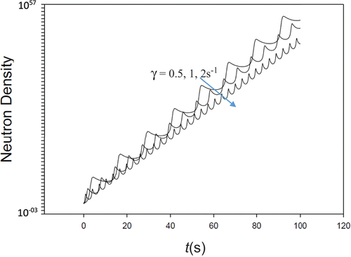
Fig. 10. (b) Neutron density for more complicated waveform.

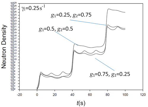
TABLE 9b1 Sine Insertion into TRIII (ρ₀ = $1, Λ = 2×10⁻⁵s, γ = 0.5s⁻¹)

t(s)	BEFD/CATS(10)	BEFD/CATS(11)	BEFD/CATS(12)	Convergence
0.0000E+00	1.0000000000E+00	1.00000000000E+00	1.000000000000E+00
1.0000E−02	1.0036278921E+00	1.00362789209E+00	1.003627892088E+00	1
1.0000E−01	1.0519635883E+00	1.05196358833E+00	1.051963588330E+00	2
1.0000E+01	2.4486238003E+06	2.44862380028E+06	2.448623800278E+06	2
5.0000E+01	1.7938198780E+26	1.79381987799E+26	1.793819877990E+26	2
7.5000E+01	2.4033270507E+39	2.40332705068E+39	2.403327050683E+39	2
1.0000E+02	3.2374576338E+52	3.23745763381E+52	3.237457633808E+52	2

As a variation, now consider the following more complicated waveform for reactivity:

(28) $\mathit{\rho }\left(\mathit{t}\right)={\rho }_0\left[g_{1}sin\left({\gamma }_1\mathit{t}\right)+g_{2}cos\left({\gamma }_2\mathit{t}\right)\right],t_{\mathit{j}-1}\le \mathit{t}\le t_j.$(28)

Taking the real part of Eq. (26a)(26a) $e^{\mathit{i\gamma t}}=\sum _{\mathit{n}=0}^{\mathrm{\infty }}{\gamma }^n\frac{i^n{e}^{\mathit{i\gamma }{\mathit{t}}_{\mathit{j}-1}}}{\mathit{n}!}{\left(\mathit{t}-{\mathit{t}}_{\mathit{j}-1}\right)}^{\mathit{n}}$(26a) gives

(29a) $cos\left(\mathit{\gamma t}\right)=\sum _{\mathit{n}=0}^{\mathrm{\infty }}\frac{{\gamma }^n}{\mathit{n}!}Re\left(i^n{e}^{\mathit{i\gamma }{\mathit{t}}_{\mathit{j}-1}}\right){\left(\mathit{t}-{\mathit{t}}_{\mathit{j}-1}\right)}^{\mathit{n}}$(29a)

to form the TS coefficient from Eqs. (26b)(26b) $sin\left(\mathit{\gamma t}\right)=\sum _{\mathit{n}=0}^{\mathrm{\infty }}\frac{{\gamma }^n}{\mathit{n}!}Im\left(i^n{e}^{\mathit{i\gamma }{\mathit{t}}_{\mathit{j}-1}}\right){\left(\mathit{t}-{\mathit{t}}_{\mathit{j}-1}\right)}^{\mathit{n}},$(26b) and (29a(29a) $cos\left(\mathit{\gamma t}\right)=\sum _{\mathit{n}=0}^{\mathrm{\infty }}\frac{{\gamma }^n}{\mathit{n}!}Re\left(i^n{e}^{\mathit{i\gamma }{\mathit{t}}_{\mathit{j}-1}}\right){\left(\mathit{t}-{\mathit{t}}_{\mathit{j}-1}\right)}^{\mathit{n}}$(29a) ):

(29b) ${\rho }_{\mathit{n},\mathit{j}-1}=\frac{{\rho }_0}{\mathit{n}!}\left[g_1{\gamma }_1^{n}Im\left(i^n{e}^{i{\gamma }_1{t}_{\mathit{j}-1}}\right)+g_2{\gamma }_2^{n}Re\left(i^n{e}^{i{\gamma }_2{t}_{\mathit{j}-1}}\right)\right].$(29b)

Assume

(30) $\begin{array}{c}{\rho }_0=\mathrm{\$}1\\ g_1=0.75\\ g_2=0.25\\ {\gamma }_1=0.5{\mathrm{s}}^{-1}\\ {\gamma }_2=0.5/\mathit{\pi }.\end{array}$(30)

In comparison with BEFD, perfect agreement results as shown in Table 9b2.

TABLE 9b2 More Complicated Sine Insertion into TRIII (ρ₀ = $1, Λ = 2x10⁻⁵s, g₁ = 0.75, g₂ = 0.25, γ₁ = 0.5s⁻¹, γ₂ = 0.5/π)

t(s)	BEFD/CATS(10)	BEFD/CATS(11)	BEFD/CATS(11)	Convergence
0.0000E+00	1.0000000000E+00	1.00000000000E+00	1.000000000000E+00
1.0000E−02	1.3140584016E+00	1.31405840163E+00	1.314058401630E+00	2
1.0000E−01	1.4201345306E+00	1.42013453061E+00	1.420134530610E+00	2
1.0000E+01	6.5775879848E+04	6.57758798483E+04	6.577587984827E+04	2
5.0000E+01	2.1229415327E+12	2.12294153270E+12	2.122941532702E+12	1
7.5000E+01	4.8634888388E+12	4.86348883880E+12	4.863488838801E+12	2
1.0000E+02	1.8785888606E+20	1.87858886056E+20	1.878588860558E+20	2

Figure 10b shows the more complicated neutron density response for the waveform of Eq. (28)(28) $\mathit{\rho }\left(\mathit{t}\right)={\rho }_0\left[g_{1}sin\left({\gamma }_1\mathit{t}\right)+g_{2}cos\left({\gamma }_2\mathit{t}\right)\right],t_{\mathit{j}-1}\le \mathit{t}\le t_j.$(28) as two superimposed waves. This opens up the possibility of Fourier series representations of reactivity with a wide range of function possibilities.

VII.A.3. Shifted Gaussian Insertion: By Recurrence

The shifted Gaussian insertion for mean μ and dispersion σ

(31) $\mathit{\rho }\left(\mathit{t}\right)=\frac{{\rho }_0}{\sqrt{2\mathit{\pi }}\mathit{\sigma }}{e}^{-{\left(\mathit{t}-\mathit{\mu }\right)}^2/2{\sigma }^2}$(31)

presents a similar challenge to the insertion of Eq. (21a)(21a) $\mathit{\rho }\left(\mathit{t}\right)={\rho }_0{e}^{\mathit{\alpha }sin\left(\mathit{\gamma t}\right)},t_{\mathit{j}-1}\le \mathit{t}\le t_j,$(21a) . Only by splitting the n’th derivative into two consecutive derivatives, one of first order

(32a) ${\rho }^{\left(\mathit{n}\right)}\left(\mathit{t}\right)=\frac{{\rho }_0}{\sqrt{2\mathit{\pi }}\mathit{\sigma }}\frac{{\mathit{d}}^{\mathit{n}-1}}{\mathit{d}{t}^{\mathit{n}-1}}\frac{d}{\mathit{dt}}{e}^{-{\left(\mathit{t}-\mathit{\mu }\right)}^2/2{\sigma }^2},$(32a)

with the first-order derivative performed explicitly, one finds

(32b) ${\rho }^{\left(\mathit{n}\right)}\left(\mathit{t}\right)=-\frac{1}{{\sigma }^2}\frac{{\mathit{d}}^{\mathit{n}-1}}{\mathit{d}{t}^{\mathit{n}-1}}\left[\left(\mathit{t}-\mathit{\mu }\right)\frac{{\rho }_0}{\sqrt{2\mathit{\pi }}\mathit{\sigma }}{e}^{-{\left(\mathit{t}-\mathit{\mu }\right)}^2/2{\sigma }^2}\right].$(32b)

Then, identifying the Gaussian reactivity in the term in brackets

(33a) ${\rho }^{\left(\mathit{n}\right)}\left(\mathit{t}\right)=-\frac{1}{{\sigma }^2}\frac{{\mathit{d}}^{\mathit{n}-1}}{\mathit{d}{t}^{\mathit{n}-1}}\left[\left(\mathit{t}-\mathit{\mu }\right)\mathit{\rho }\left(\mathit{t}\right)\right]$(33a)

and from Leibnitz’s product differentiation

(33b) ${\rho }^{\left(\mathit{n}\right)}\left(\mathit{t}\right)=-\frac{1}{{\sigma }^2}\sum _{\mathit{l}=0}^{\mathit{n}-1}\frac{\left(\mathit{n}-1\right)!}{\mathit{l}!\left(\mathit{n}-1-\mathit{l}\right)!}\left[\frac{d^l}{\mathit{d}{t}^l}\left(\mathit{t}-\mathit{\mu }\right)\right]{\rho }^{\left(\mathit{n}-1-\mathit{l}\right)}\left(\mathit{t}\right),$(33b)

there results the following recurrence at t = t_j–1:

(33c) ${\rho }_{j-1}^{\left(n\right)}\equiv {\rho }_{\mathit{n},\mathit{j}-1}=-\frac{1}{{\sigma }^2}\left[\left(t_{\mathit{j}-1}-\mathit{\mu }\right){\rho }_{j-1}^{\left(n-1\right)}+\left(\mathit{n}-1\right){\rho }_{j-1}^{\left(n-2\right)}\right],$(33c)

or the TS coefficient by recurrence is

(33d) ${\rho }_{\mathit{n},\mathit{j}-1}=-\frac{1}{n{\sigma }^2}\left[\left(t_{\mathit{j}-1}-\mathit{\mu }\right){\rho }_{\mathit{n}-1,\mathit{j}-1}+{\rho }_{\mathit{n}-2,\mathit{j}-1}\right]$(33d)

initiated by

(33e) ${\rho }_{0,\mathit{j}}=\frac{{\rho }_0}{\sqrt{2\mathit{\pi }}\mathit{\sigma }}{e}^{-{\left(t_j-\mathit{\mu }\right)}^2/2{\sigma }^2}.$(33e)

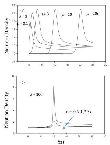
Table 9c shows the comparison for a shifted Gaussian reactivity centered about μ = 3 with dispersion of unity and ρ₀ = $1. We see perfect agreement to 12 places for the nominal case.

TABLE 9c Shifted Gaussian Insertion for TRIII (ρ₀ = $1, Λ = 2×10⁻⁵s, μ = 3s, σ = 1s)

t(s)	BEFD/CATS(10)	BEFD/CATS(11)	BEFD/CATS(12)	Convergence
0.0000E+00	1.0000000000E+00	1.00000000000E+00	1.000000000000E+00
1.0000E−02	1.0044221872E+00	1.00442218720E+00	1.004422187197E+00	2
1.0000E−01	1.0061403508E+00	1.00614035081E+00	1.006140350815E+00	2
1.0000E+00	1.0646324990E+00	1.06463249900E+00	1.064632498998E+00	2
1.0000E+01	1.2421861201E+00	1.24218612010E+00	1.242186120104E+00	2
2.0000E+01	1.1814969337E+00	1.18149693366E+00	1.181496933662E+00	2
2.5000E+01	1.1690820343E+00	1.16908203429E+00	1.169082034289E+00	2

Figure 11a shows a pulse advancing in time centered from 0.1 to 20s with ρ₀ = $1. Apparently, the pulse reaches a fixed shape at sufficiently long time. In contrast, Fig. 11b shows the dispersion of a fixed pulse centered at t = 10s with σ ranging from 0.5 to 3s forcing the pulse height to increase with decreasing dispersion since the Gaussian is constant on integration.

Fig. 11. (a) Gaussian insertion for μ = 0.1, 1, 3, 10, 20s and σ = 1s in TRIII. (b) Dispersion reduction for σ = 0.5, 1, 2, 3s for μ = 10s.

VII.A.4. Bessel Function Insertion: From the Literature

For the last example for this section, we consider a zeroth-order Bessel function insertion

(34) $\mathit{\rho }\left(\mathit{t}\right)={\rho }_0{J}_0\left(\mathit{\alpha t}\right).$(34)

This unusual insertion whose n’th derivative for m = 0 comes from the literature^[31]

(35a) ${\rho }_j^{\left(n\right)}=\frac{d^n{J}_m\left(\mathit{\alpha t}\right)}{\mathit{d}{t}^n}={\rho }_0{\left[\frac{\alpha }{2}\right]}^{\mathit{n}}\sum _{\mathit{k}=0}^n{\left(-1\right)}^k\left(\begin{array}{c}\mathit{n}\\ \mathit{k}\end{array}\right)J_{2\mathit{k}-\mathit{n}+\mathit{m}}\left(\mathit{\alpha t}\right)$(35a)

gives the TS coefficient when m = 0:

(35b) ${\rho }_{\mathit{n},\mathit{j}}=\frac{1}{\mathit{n}!}{\left.\frac{d^n{J}_0\left(\mathit{\alpha t}\right)}{\mathit{d}{t}^n}\right|}_{t_j}=\frac{{\rho }_0}{\mathit{n}!}{\left[\frac{\alpha }{2}\right]}^{\mathit{n}}\sum _{\mathit{k}=0}^n{\left(-1\right)}^k\left(\begin{array}{c}\mathit{n}\\ \mathit{k}\end{array}\right)J_{2\mathit{k}-\mathit{n}}\left(\mathit{\alpha }{t}_j\right).$(35b)

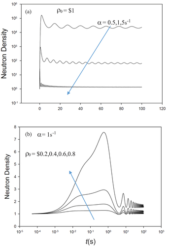
On comparison with BEFD, we see only one discrepancy in the 12th place for α = 1 and ρ₀ = $0.2 shown in Table 9d.

TABLE 9d Bessel Function Insertion for TRIII (ρ₀ = $0.2, Λ = 2×10⁻⁵s, α = 1s⁻¹)

t(s)	BEFD/CATS(10)	BEFD/CATS(11)	BEFD/CATS(12)	Convergence
0.0000E+00	1.0000000000E+00	1.00000000000E+00	1.000000000000E+00
1.0000E−02	1.2353216419E+00	1.23532164189E+00	1.235321641890E+00	2
1.0000E−01	1.2613107936E+00	1.26131079362E+00	1.261310793617E+00	1
1.0000E+00	1.2648939690E+00	1.26489396900E+00	1.264893969004E+00	2
1.0000E+01	9.8636673361E−01	9.86366733608E−01	9.863667336081E−01	1
1.0000E+02	1.0261817333E+00	1.02618173332E+00	1.02618173332E+00	1

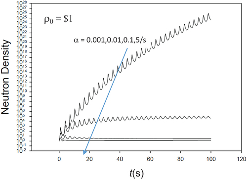
Figure 12a shows the increase in the frequency of oscillation in time with decreasing α and for $1 insertion. The oscillations come from the functional behavior of the Bessel function. In Fig. 12b, we see a growing first pulse followed by smaller pulses increasing in amplitude with reactivity. Note that any order Bessel function can be a reactivity.

Fig. 12. (a) Bessel function oscillations in time for ρ₀ = $1 with α = 0.5, 1, 5s⁻¹. (b) Increase in density response with reactivity for ρ₀ = $0.2, 0.4, 0.6, 0.8 with α = 1s⁻¹.

VII.B. Combination Reactivity Insertions into TRIII

The following set of insertions takes the form

(36a) $\mathit{\rho }\left(\mathit{t}\right)={\rho }_0\mathit{f}\left(\mathit{t}\right)\mathit{g}\left(\mathit{t}\right),$(36a)

which from Leibnitz’s differentiation most conveniently gives the derivative

(36b) ${\rho }^{\left(\mathit{n}\right)}\left(\mathit{t}\right)={\rho }_0\sum _{\mathit{l}=0}^n\frac{\mathit{n}!}{\mathit{l}!\left(\mathit{n}-\mathit{l}\right)!}{f}^{(\mathit{n}-\mathit{l})}\left(\mathit{t}\right)g^{\left(\mathit{l}\right)}\left(\mathit{t}\right).$(36b)

Therefore, the TS coefficient of reactivity for the combination becomes at t_j

(37) ${\rho }_{\mathit{n},\mathit{j}}={\rho }_0\sum _{\mathit{l}=0}^n{f}_{\mathit{n}-\mathit{l},\mathit{j}}{g}_{\mathit{l},\mathit{j}}$(37)

to be introduced into Eq(4a)(4a,b) $\begin{array}{rl}& \left(\mathit{n}+1\right)N_{\mathit{n}+1,\mathit{j}}=\frac{1}{\mathrm{\Lambda }}{\gamma }_{\mathit{n},\mathit{j}}+\sum _{\mathit{i}=0}^m{\lambda }_i{C}_{\mathit{i},\mathit{n},\mathit{j}}\\ & \left(\mathit{n}+1\right)C_{\mathit{i},\mathit{n}+1,\mathit{j}}=\frac{{\beta }_i}{\mathrm{\Lambda }}{N}_{\mathit{n},\mathit{j}}-{\lambda }_i{C}_{\mathit{i},\mathit{n},\mathit{j}}.\end{array}$(4a,b) .

VII.B.1. Oscillating/Exponential Insertion

The oscillating exponentially damped insertion is

(38a) $\mathit{\rho }\left(\mathit{t}\right)={\rho }_{0}sin\left(\mathit{\gamma t}\right)e^{-\mathit{\alpha t}}$(38a)

for which

(38b) $\mathit{f}\left(\mathit{t}\right)=sin\left(\mathit{\gamma t}\right),\mathit{g}(\mathit{t})=e^{-\mathit{\alpha t}}.$(38b)

However, before applying Eq. (38a)(38a) $\mathit{\rho }\left(\mathit{t}\right)={\rho }_{0}sin\left(\mathit{\gamma t}\right)e^{-\mathit{\alpha t}}$(38a) directly in Eq. (37(37) ${\rho }_{\mathit{n},\mathit{j}}={\rho }_0\sum _{\mathit{l}=0}^n{f}_{\mathit{n}-\mathit{l},\mathit{j}}{g}_{\mathit{l},\mathit{j}}$(37) ), the following alternative as applied previously simplifies the derivation of the TS coefficient.

Since the insertion is equivalent to

(39a) $\mathit{\rho }\left(\mathit{t}\right)={\rho }_{0}Im{e}^{\mathit{i\gamma t}}{e}^{-\mathit{\alpha t}},$(39a)

combination of the exponentials gives

(39b) $\mathit{\rho }\left(\mathit{t}\right)={\rho }_{0}Im{e}^{\mathit{i\gamma t}-\mathit{\alpha t}}$(39b)

and on differentiation

(39c) ${\rho }^{(\mathit{n})}\left(\mathit{t}\right)={\rho }_{0}Im\left({\left(-1\right)}^n{\left(\mathit{\alpha }-\mathit{i\gamma }\right)}^n{e}^{-\left(\mathit{\alpha }-\mathit{i\gamma }\right)t}\right).$(39c)

With simplification, the TS coefficient at t_j becomes

(40) ${\rho }_{\mathit{n},\mathit{j}}={\rho }_0\frac{{\left(-1\right)}^n}{\mathit{n}!}{\left({\alpha }^2+{\gamma }^2\right)}^{\mathit{n}/2}sin\left(\mathit{\gamma }{t}_j-\mathit{n}{tan}^{-1}\left(\mathit{\gamma }/\mathit{\alpha }\right)\right)e^{-\alpha t_j}.$(40)

Again, we find perfect agreement as shown in Table 10a and observe the oscillations of Fig. 13, which shows the influence of the exponential factor of the insertion to suppress the increase caused by the sine factor.

TABLE 10a Oscillating/Exponential Insertion in TRIII (ρ₀ = $1, Λ = 2×10⁻⁵s, α = 0.1s⁻¹, γ = 2s⁻¹)

t(s)	BEFD/CATS(10)	BEFD/CATS(11)	BEFD/CATS(12)	Convergence
0.0000E+00	1.0000000000E+00	1.00000000000E+00	1.000000000000E+00
1.0000E−02	1.0146190215E+00	1.01461902149E+00	1.014619021486E+00	2
1.0000E−01	1.2396514745E+00	1.23965147446E+00	1.239651474460E+00	2
1.0000E+01	6.1311855874E+00	6.13118558741E+00	6.131185587406E+00	2
5.0000E+01	3.0355853322E+00	3.03558533219E+00	3.035585332191E+00	2
1.0000E+02	2.9453018081E+00	2.94530180809E+00	2.945301808091E+00	2

Fig. 13. Oscillating/exponential insertion in TRIII.

Now, back to the original form of Eq. (36a)(36a) $\mathit{\rho }\left(\mathit{t}\right)={\rho }_0\mathit{f}\left(\mathit{t}\right)\mathit{g}\left(\mathit{t}\right),$(36a) with application of Leibnitz’s differentiation, we find from Eq. (37(37) ${\rho }_{\mathit{n},\mathit{j}}={\rho }_0\sum _{\mathit{l}=0}^n{f}_{\mathit{n}-\mathit{l},\mathit{j}}{g}_{\mathit{l},\mathit{j}}$(37) ),

(41a) $f_{\mathit{n},\mathit{j}}=\frac{{\gamma }^n}{\mathit{n}!}Im\left(i^n{e}^{i\gamma t_j}\right)$(41a)

(41b) $g_{\mathit{n},\mathit{j}}=\frac{{\left(-1\right)}^n}{\mathit{n}!}{\alpha }^n{e}^{-\alpha t_j},\mathit{\hspace{0.17em}}\mathit{n}=0,1,...,$(41b)

and therefore from Eq. (37(37) ${\rho }_{\mathit{n},\mathit{j}}={\rho }_0\sum _{\mathit{l}=0}^n{f}_{\mathit{n}-\mathit{l},\mathit{j}}{g}_{\mathit{l},\mathit{j}}$(37) ), ${\rho }_{\mathit{n},\mathit{j}}$ is

(42) ${\rho }_{\mathit{n},\mathit{j}}={\rho }_0{e}^{-\alpha t_j}\sum _{\mathit{l}=0}^n{\left(-1\right)}^l{\alpha }^l\frac{{\mathit{\gamma }}^{\mathit{n}-\mathit{l}}}{\mathit{l}!\left(\mathit{n}-\mathit{l}\right)!}sin\left(\mathit{\gamma }{t}_j+\frac{\pi }{2}\left(\mathit{n}-\mathit{l}\right)\right)$(42)

which gives identical results (not shown) as Table 10a.

VII.B.2. Oscillating/Shifted-Gaussian/Exponential Insertion

A more complicated reactivity involves sine, Gaussian, and exponential factors

(43a) $\mathit{\rho }\left(\mathit{t}\right)={\rho }_0\mathit{f}\left(\mathit{t}\right)\mathit{g}\left(\mathit{t}\right)\mathit{h}\left(\mathit{t}\right),$(43a)

where

(43b) $\mathit{f}\left(\mathit{t}\right)=sin\left(\mathit{\gamma t}\right),\mathit{g}(\mathit{t})=e^{-\mathit{\gamma t}},\mathit{h}(\mathit{t})=\frac{{\mathit{e}}^{-{\left(\mathit{t}-\mathit{\mu }\right)}^2/2{\sigma }^2}}{\sqrt{2\mathit{\pi }}\mathit{\sigma }}.$(43b)

From the previous example, one application of Leibnitz’s differentiation gives the TS coefficient for f(t)g(t) as

(44a) $s_{\mathit{n},\mathit{j}}\equiv \sum _{\mathit{l}=0}^n{f}_{\mathit{n}-\mathit{l},\mathit{j}}{g}_{\mathit{l},\mathit{j}},$(44a)

where

(44b) $f_{\mathit{n},\mathit{j}}=\frac{{\gamma }^n}{\mathit{n}!}Im\left(i^n{e}^{i\gamma t_j}\right)$(44b)

(44c) $g_{\mathit{n},\mathit{j}}=\frac{{\left(-1\right)}^n}{\mathit{n}!}{\alpha }^n{e}^{-\alpha t_j}.$(44c)

A second application of Leibnitz’s differentiation then gives the triple product reactivity associated with Eqs. (43a)(43a) $\mathit{\rho }\left(\mathit{t}\right)={\rho }_0\mathit{f}\left(\mathit{t}\right)\mathit{g}\left(\mathit{t}\right)\mathit{h}\left(\mathit{t}\right),$(43a) and (43b(43b) $\mathit{f}\left(\mathit{t}\right)=sin\left(\mathit{\gamma t}\right),\mathit{g}(\mathit{t})=e^{-\mathit{\gamma t}},\mathit{h}(\mathit{t})=\frac{{\mathit{e}}^{-{\left(\mathit{t}-\mathit{\mu }\right)}^2/2{\sigma }^2}}{\sqrt{2\mathit{\pi }}\mathit{\sigma }}.$(43b) ) as

(45) ${\rho }_{\mathit{n},\mathit{j}}\equiv {\rho }_0\sum _{\mathit{l}=0}^n{s}_{\mathit{n}-\mathit{l},\mathit{j}}{h}_{\mathit{l},\mathit{j}},$(45)

where h_l,_j is the recurrence for the Shifted-Gaussian distribution found in Sec. VII.A.3. Table 10b confirms all places of CATS relative to BEFD. For a Gaussian pulse centered at 5s with a spread of 1s, Fig. 14 shows the imprinted oscillations over the pulse width.

Fig. 14. Imprinted oscillations over the pulse width.

TABLE 10b Oscillating/Gaussian/Exponential Insertion for TRIII (ρ₀ = $1, Λ = 2×10⁻⁵s, α = 0.01s⁻¹, σ = 1s, μ = 5, γ = 20s⁻¹)

t(s)	BEFD/CATS(10)	BEFD/CATS(11)	BEFD/CATS(12)	Convergence
0.0000E+00	1.0000000000E+00	1.00000000000E+00	1.000000000000E+00
1.0000E−02	1.0000002230E+00	1.00000022302E+00	1.000000223022E+00	1
1.0000E−01	1.0000022892E+00	1.00000228916E+00	1.000002289161E+00	1
5.0000E+00	8.4047931778E−01	8.40479317785E−01	8.404793177847E−01	2
1.0000E+01	1.0215505490E+00	1.02155054897E+00	1.021550548969E+00	2
1.5000E+01	1.0173288001E+00	1.01732880011E+00	1.017328800110E+00	2

VIII. VARIATIONS ON DOPPLER FEEDBACK

In this section, we consider several generalizations with the Doppler effect for step reactivity. The generalizations admit TS for reactivity that conform to the CATS algorithm. The variations are similar to Secs. VI.A and VI.B but are more sophisticated, and therefore, one should not expect the 10- or 11-place results of the previous benchmarks to be as readily produced. All examples will be for Thermal Reactor IV with kinetic parameters from Table A.V in Appendix A.

VIII.A. Doppler Feedback: Internal Factor

We first consider a modified Doppler feedback with an internal factor f(t) in the Doppler term

(46) $\mathit{\rho }\left(\mathit{t}\right)={\rho }_0-\mathit{B}\underset{0}{\overset{t}{\int }}\mathit{dt}{ }^{\mathrm{\prime }}\mathit{f}\left(\mathit{t}{ }^{\mathrm{\prime }}\right)\mathit{N}\left(\mathit{t}{ }^{\mathrm{\prime }}\right).$(46)

One proceeds as before by finding the n’th derivative of the reactivity according to

(47a) ${\rho }^{\left(\mathit{n}\right)}\left(\mathit{t}\right)=\frac{{\mathit{d}}^{\mathit{n}-1}}{\mathit{d}{t}^{\mathit{n}-1}}\frac{\mathit{d\rho }\left(\mathit{t}\right)}{\mathit{dt}}=-\mathit{B}\frac{{\mathit{d}}^{\mathit{n}-1}}{\mathit{d}{t}^{\mathit{n}-1}}\mathit{f}\left(\mathit{t}\right)\mathit{N}\left(\mathit{t}\right)$(47a)

to give

(47b) ${\rho }^{\left(\mathit{n}\right)}\left(\mathit{t}\right)={\rho }_0{\delta }_{\mathit{n},0}-\mathit{B}\sum _{\mathit{l}=0}^{\mathit{n}-1}\frac{\left(\mathit{n}-1\right)!}{\mathit{l}!\left(\mathit{n}-1-\mathit{l}\right)!}{f}^{\left(\mathit{n}-1-\mathit{l}\right)}\left(\mathit{t}\right)N^{\left(\mathit{l}\right)}\left(\mathit{t}\right).$(47b)

The TS coefficient is therefore

(48) ${\rho }_{\mathit{n},\mathit{j}-1}={\rho }_0{\delta }_{\mathit{n},0}-\frac{B}{n}\sum _{\mathit{l}=0}^{\mathit{n}-1}{f}_{\mathit{n}-1-\mathit{l},\mathit{j}-1}{N}_{\mathit{l},\mathit{j}-1}.$(48)

As a demonstration, we consider several factors with step reactivity insertion.

VIII.A.1. Exponential Factor

If

(49a) $\mathit{f}\left(\mathit{t}\right)\equiv e^{-\mathit{\alpha t}},$(49a)

then

(49b) $f_n=\frac{{\left(-1\right)}^n}{\mathit{n}!}{\alpha }^n{e}^{-\mathit{\alpha t}},$(49b)

and the TS coefficient for reactivity becomes

(49c) ${\rho }_{\mathit{n},\mathit{j}-1}={\rho }_0{\delta }_{\mathit{n},0}-\frac{B}{n}{e}^{-\mathit{\alpha }{\mathit{t}}_{\mathit{j}-1}}{\displaystyle \sum _{\mathit{l}=0}^{\mathit{n}-1}{\left(-1\right)}^{\left(\mathit{n}-1-\mathit{l}\right)}\frac{{\mathit{\alpha }}^{\left(\mathit{n}-1-\mathit{l}\right)}}{\left(\mathit{n}-1-\mathit{l}\right)!}}{N}_{\mathit{l},\mathit{j}-1}$(49c)

with Doppler exponent α = 0.1s⁻¹. Table 11a1 shows no discrepancies for 9 or 10 places for the NIPL with l2 set to 12 to give a greater possibility for convergence within the partitions. In the 11th place, two entries do not conform. When l2 is set to 15, only the second discrepancy remains. Further wrangling did not work in this case, so we accept the 10-place benchmark.

TABLE 11a1 Doppler Feedback with an Internal Exponential Factor (ρ₀ = 0.1, Λ = 5×10⁻⁵s, α = 0.1s⁻¹)

t(s)	BEFD/CATS(9)	BEFD/CATS(10)	BEFD/CATS(11)
0.0000E+00	1.000000000E+00	1.0000000000E+00	1.00000000000E+00
1.0000E+00	1.146784429E+00	1.1467844285E+00	1.14678442851E+00
1.0000E+01	1.332167947E+00	1.3321679468E+00	1.33216794681E+00
2.0000E+01	1.500952047E+00	1.5009520468E+00	1.50095204684E+00
3.0000E+01	1.668934194E+00	1.6689341938E+00	1.66893419381E+00
4.0000E+01	1.846248311E+00	1.8462483107E+00	1.84624831075E+00
5.0000E+01	2.037493519E+00	2.0374935191E+00	2.03749351915E+00
6.0000E+01	2.245722110E+00	2.2457221099E+00	2.24572210988E+00
7.0000E+01	2.473470810E+00	2.4734708104E+00	2.47347081040E+00
8.0000E+01	2.723138348E+00	2.7231383483E+00	2.72313834826E+00
9.0000E+01	2.997163664E+00	2.9971636640E+00	2.99716366400E+00
1.0000E+02	3.298124366E+00	3.2981243655E+00	3.29812436554E+00

Figure 15 shows how α enables control of the Doppler effect to shut down the step transient. For α > 0, Doppler dies away relatively quickly and offers minimal transient reduction. For α < 0, the Doppler term is larger and when sufficiently large provides enough negative reactivity to turn the transient around. To the author’s knowledge, showing control of the Doppler in this way is new.

Fig. 15. Doppler control through α.

VIII.A.2. Sine Factor

For

(50a) $\mathit{f}\left(\mathit{t}\right)\equiv sin\left(\mathit{\gamma t}\right),$(50a)

then

(50b) $f_n\left(\mathit{t}\right)=sin\left(\mathit{\gamma t}+\mathit{\pi n}/2\right),$(50b)

and the TS coefficient with Doppler is

(50c) $\begin{array}{rl}& {\rho }_{\mathit{n},\mathit{j}-1}={\rho }_0{\delta }_{\mathit{n},0}-\frac{B}{n}\sum _{\mathit{l}=0}^{\mathit{n}-1}\frac{{\mathit{\gamma }}^{\left(\mathit{n}-1-\mathit{l}\right)}}{\left(\mathit{n}-1-\mathit{l}\right)!}\\ & sin\left(\mathit{\gamma t}+\mathit{\pi }\left(\mathit{n}-1-\mathit{l}\right)/2\right)N_{\mathit{l},\mathit{j}-1}.& (50\mathrm{c})\end{array}$(50c)

Table 11a2 indicates that NIPL for err of 10⁻¹² and l2 at 12 have no discrepancies for 9 and 10 places, but four occur for 11 places. Most notably, when err is set to 10⁻¹³, all 11 places now agree.

TABLE 11a2 Doppler Feedback with an Internal Sine Factor (ρ₀ = 0.2, Λ = 5×10⁻⁵s, γ = 5s⁻¹, B = 2.5×10⁻⁶/MWs)

t(s)	BEFD/CATS(9)	BEFD/CATS(10)	BEFD/CATS(11)
0.0000E+00	1.000000000E+00	1.0000000000E+00	1.00000000000E+00
1.0000E+00	1.343645243E+00	1.3436452430E+00	1.34364524297E+00
1.0000E+01	1.936737853E+00	1.9367378533E+00	1.93673785328E+00
2.0000E+01	2.647546946E+00	2.6475469456E+00	2.64754694562E+00
4.0000E+01	4.667892768E+00	4.6678927677E+00	4.6678927677E+00
6.0000E+01	8.076561475E+00	8.0765614747E+00	8.07656147474E+00
8.0000E+01	1.391093956E+01	1.3910939558E+01	1.39109395584E+01
1.0000E+02	2.391730138E+01	2.3917301378E+01	2.39173013782E+01

Figure 16 shows how the $0.6 reactivity insertion shuts down with a sine factor of frequency 3 coupled to a decreasing Doppler coefficient. The power oscillation is a unique feature of the sine reactivity trace.

Fig. 16. Doppler shut down by sine internal factor.

VIII.B. Doppler Feedback: External Factor

As another variation, consider the factor external to the Doppler term:

(51) $\mathit{\rho }\left(\mathit{t}\right)={\rho }_0-\mathit{Bf}\left(\mathit{t}\right)\underset{0}{\overset{t}{\int }}\mathit{dt}{ }^{\mathrm{\prime }}\mathit{N}\left(\mathit{t}{ }^{\mathrm{\prime }}\right).$(51)

Separating the integral into past and current Doppler contributions,

(52a) $\mathit{\rho }\left(\mathit{t}\right)={\rho }_0-\mathit{Bf}\left(\mathit{t}\right)\left[\underset{0}{\overset{{\mathit{t}}_{\mathit{j}-1}}{\int }}\mathit{dt}{ }^{\mathrm{\prime }}\mathit{N}\left(\mathit{t}{ }^{\mathrm{\prime }}\right)+\underset{{\mathit{t}}_{\mathit{j}-1}}{\overset{\mathit{t}}{\int }}\mathit{dt}{ }^{\mathrm{\prime }}\mathit{N}\left(\mathit{t}{ }^{\mathrm{\prime }}\right)\right],$(52a)

and noting that when t = t_j–1,

(52b) $-\mathit{B}\underset{0}{\overset{{\mathit{t}}_{\mathit{j}-1}}{\int }}\mathit{dt}{ }^{\mathrm{\prime }}\mathit{N}\left(\mathit{t}{ }^{\mathrm{\prime }}\right)=-\frac{{\rho }_0-\mathit{\rho }\left(t_{\mathit{j}-1}\right)}{\mathit{f}\left(t_{\mathit{j}-1}\right)}$(52b)

gives

(52c) $\begin{array}{rl}& \mathit{\rho }\left(\mathit{t}\right)={\rho }_0-\frac{\mathit{f}\left(\mathit{t}\right)}{\mathit{f}\left({\mathit{t}}_{\mathit{j}-1}\right)}\left[{\rho }_0-\mathit{\rho }\left(t_{\mathit{j}-1}\right)\right]-\\ & -\mathit{Bf}\left(\mathit{t}\right)\underset{{\mathit{t}}_{\mathit{j}-1}}{\overset{\mathit{t}}{\int }}\mathit{dt}{ }^{\mathrm{\prime }}\mathit{N}\left(\mathit{t}{ }^{\mathrm{\prime }}\right).& (52\mathrm{c})\end{array}$(52c)

On differentiating n times by application of Leibnitz’s formula,

(53a) ${\rho }^{\left(\mathit{n}\right)}\left(\mathit{t}\right)={\rho }_0{\delta }_{\mathit{n},0}-\frac{{\mathit{f}}^{\left(\mathit{n}\right)}\left(\mathit{t}\right)}{\mathit{f}\left(t_{\mathit{j}-1}\right)}\left[{\rho }_0-\mathit{\rho }\left(t_{\mathit{j}-1}\right)\right]--\mathit{B}{\displaystyle \sum _{\mathit{l}=0}^n\frac{\mathit{n}!}{\mathit{l}!\left(\mathit{n}-\mathit{l}\right)!}}{f}^{\left(\mathit{n}-\mathit{l}\right)}\left(\mathit{t}\right)\frac{d^l}{\mathit{d}{t}^l}\int t_{\mathit{j}-1}\mathit{t}\mathit{dt}\prime \mathit{Nt}\prime .(\text{53a})$(53a)

Separating out the first term of the sum and from Eq (14b(14b) $\frac{d^n}{\mathit{d}{t}^n}\underset{0}{\overset{t}{\int }}\mathit{dt}{ }^{\mathrm{\prime }}\mathit{N}\left(\mathit{t}{ }^{\mathrm{\prime }}\right)=\frac{{\mathit{d}}^{\mathit{n}-1}}{\mathit{d}{t}^{\mathit{n}-1}}\frac{d}{\mathit{dt}}\underset{0}{\overset{t}{\int }}\mathit{dt}{ }^{\mathrm{\prime }}\mathit{N}\left(\mathit{t}{ }^{\mathrm{\prime }}\right)=N^{\left(\mathit{n}-1\right)}\left(\mathit{t}\right),$(14b) ), there results

(53b) $\begin{array}{rl}& {\rho }^{\left(\mathit{n}\right)}\left(\mathit{t}\right)={\rho }_0{\delta }_{\mathit{n},0}-\frac{{\mathit{f}}^{\left(\mathit{n}\right)}\left(\mathit{t}\right)}{\mathit{f}\left(t_{\mathit{j}-1}\right)}\left[{\rho }_0-\mathit{\rho }\left(t_{\mathit{j}-1}\right)\right]-\\ & -\mathit{B}\sum _{\mathit{l}=1}^n\frac{\mathit{n}!}{\mathit{l}!\left(\mathit{n}-\mathit{l}\right)!}{f}^{\left(\mathit{n}-\mathit{l}\right)}\left(\mathit{t}\right)N^{\left(\mathit{l}-1\right)}\left(\mathit{t}\right)-\\ & -\mathit{B}{f}^{\left(\mathit{n}\right)}\left(\mathit{t}\right)\underset{{\mathit{t}}_{\mathit{j}-1}}{\overset{\mathit{t}}{\int }}\mathit{dt}{ }^{\mathrm{\prime }}\mathit{N}\left(\mathit{t}{ }^{\mathrm{\prime }}\right).& (53\mathrm{b})\end{array}$(53b)

By definition,

(54a) $\mathit{\rho }\left(t_{\mathit{j}-1}\right)\equiv {\rho }_{0,\mathit{j}-1},$(54a)

and at t = t_j–1,

(54b) $\begin{array}{rl}& {\rho }_{\mathit{n},\mathit{j}-1}={\rho }_0{\delta }_{\mathit{n},0}-\frac{{\mathit{f}}_{\mathit{n},\mathit{j}-1}}{f_{0,\mathit{j}-1}}\left[{\rho }_0-{\rho }_{0,\mathit{j}-1}\right]-\\ & -\mathit{B}\sum _{\mathit{l}=1}^n\frac{1}{l}{f}_{\mathit{n}-\mathit{l},\mathit{j}-1}{N}_{\mathit{l}-1,\mathit{j}-1}.\end{array}$(54b)

Now, we demonstrate several external factors.

VIII.B.1. External Exponential Factor

If

(55a) $\mathit{f}\left(\mathit{t}\right)\equiv e^{-\mathit{\alpha t}},$(55a)

then

(55b) $f^{\left(\mathit{n}\right)}\left(\mathit{t}\right)=\frac{{\left(-1\right)}^n}{\mathit{n}!}{\alpha }^n{e}^{-\mathit{\alpha t}},$(55b)

and the TS coefficient for reactivity is

(55c) $\begin{array}{rl}& {\rho }_{\mathit{n},\mathit{j}-1}={\rho }_0{\delta }_{\mathit{n},0}-\frac{{\left(-1\right)}^{\mathit{n}-1}}{\mathit{n}!}{\alpha }^n{e}^{-\mathit{\alpha }{\mathit{t}}_{\mathit{j}-1}}\left[{\rho }_0-{\rho }_{0,\mathit{j}-1}\right]-\\ & -\mathit{B}{e}^{-\mathit{\alpha }{\mathit{t}}_{\mathit{j}-1}}\sum _{\mathit{l}=1}^n{\left(-1\right)}^{\left(\mathit{n}-\mathit{l}\right)}\frac{{\mathit{\alpha }}^{\left(\mathit{n}-\mathit{l}\right)}}{\mathit{l}\left(\mathit{n}-\mathit{l}\right)!}{N}_{\mathit{l}-1,\mathit{j}-1}.& (55\mathrm{c})\end{array}$(55c)

Table 11b1 indicates four discrepancies in the 11th place for err set to 10⁻¹¹, but when set to 3 × 10⁻¹², all discrepancies disappear. Figure 17 shows the control of the Doppler.

Fig. 17. Doppler control through α for external exponential factor.

TABLE 11b1 Doppler Feedback with an External Exponential Factor (ρ₀ = 0.1, Λ = 5×10⁻⁵s, α = 1s⁻¹, B = 2.5×10⁻⁶/MWs)

t(s)	BEFD/CATS(9)	BEFD/CATS(10)	BEFD/CATS(11)
0.0000E+00	1.000000000E+00	1.0000000000E+00	1.00000000000E+00
1.0000E+00	1.147148287E+00	1.1471482871E+00	1.14714828712E+00
1.0000E+01	1.341891344E+00	1.3418913444E+00	1.34189134439E+00
2.0000E+01	1.524321242E+00	1.5243212420E+00	1.52432124196E+00
4.0000E+01	1.903306872E+00	1.9033068715E+00	1.9033068715E+00
6.0000E+01	2.347276140E+00	2.3472761398E+00	2.3472761398E+00
8.0000E+01	2.884599866E+00	2.8845998660E+00	2.8845998660E+00
1.0000E+02	3.540257001E+00	3.5402570007E+00	3.5402570007E+00

VIII.B.2. External Gaussian Factor

For

(56a) $\mathit{f}\left(\mathit{t}\right)\equiv e^{-\alpha t^2},$(56a)

then

(56b) $f^{\left(\mathit{n}\right)}\left(\mathit{t}\right)=-2\mathit{\alpha }\frac{{\mathit{d}}^{\mathit{n}-1}}{\mathit{d}{t}^{\mathit{n}-1}}\mathit{t}{e}^{-\alpha t^2},$(56b)

which gives the recurrence

(56c) $f_{\mathit{n},\mathit{j}-1}=-\frac{2\mathit{\alpha }}{n}\left(t_{\mathit{j}-1}{f}_{\mathit{n}-1,\mathit{j}-1}+f_{\mathit{n}-2,\mathit{j}-1}\right),$(56c)

initiated by

(56d) $f_{0.\mathit{j}-1}=-2\mathit{\alpha }{e}^{-\alpha t_{j-1}^2}.$(56d)

The TS coefficient with Doppler is Eq. (54b)(54b) $\begin{array}{rl}& {\rho }_{\mathit{n},\mathit{j}-1}={\rho }_0{\delta }_{\mathit{n},0}-\frac{{\mathit{f}}_{\mathit{n},\mathit{j}-1}}{f_{0,\mathit{j}-1}}\left[{\rho }_0-{\rho }_{0,\mathit{j}-1}\right]-\\ & -\mathit{B}\sum _{\mathit{l}=1}^n\frac{1}{l}{f}_{\mathit{n}-\mathit{l},\mathit{j}-1}{N}_{\mathit{l}-1,\mathit{j}-1}.\end{array}$(54b) .

All digits to 11 places agree as shown in Table 11b2 for NIPL with l2 set to 12 and m1 set to 1. Figure 18 shows a much faster shutdown of the transient for the Gaussian factor than for the exponential.

TABLE 11b2 Doppler Feedback with an External Gaussian Factor (ρ₀ = 0.1, Λ = 5×10⁻⁵s α = 0.1s⁻¹, B = 2.5×10⁻⁶/MWs)

t(s)	BEFD/CATS(9)	BEFD/CATS(10)	BEFD/CATS(11)
0.0000E+00	1.000000000E+00	1.0000000000E+00	1.00000000000E+00
1.0000E+00	1.146811100E+00	1.1468111005E+00	1.14681110050E+00
1.0000E+01	1.341459632E+00	1.3414596325E+00	1.34145963249E+00
2.0000E+01	1.523933344E+00	1.5239333435E+00	1.52393334353E+00
4.0000E+01	1.902881669E+00	1.9028816688E+00	1.90288166882E+00
6.0000E+01	2.346768735E+00	2.3467687351E+00	2.34676873510E+00
8.0000E+01	2.883983064E+00	2.8839830641E+00	2.88398306409E+00
1.0000E+02	3.539503427E+00	3.5395034268E+00	3.53950342681E+00

Fig. 18. Doppler shutdown for Gaussian factor.

VIII.B.3. External Exponential/Sine Factor

For

(57a) $\mathit{f}\left(\mathit{t}\right)\equiv e^{\mathit{\alpha }sin\left(\mathit{\gamma t}\right)},$(57a)

then from Eq. (22b(22b) ${\rho }^{\left(\mathit{n}\right)}\left(\mathit{t}\right)={\rho }_0\mathit{\alpha \gamma }\sum _{\mathit{l}=0}^{\mathit{n}-1}\frac{\left(\mathit{n}-1\right)!}{\mathit{l}!\left(\mathit{n}-1-\mathit{l}\right)!}\frac{{\mathit{d}}^{\mathit{n}-1-\mathit{l}}cos\left(\mathit{\gamma t}\right)}{\mathit{d}{t}^{\mathit{n}-1-\mathit{l}}}{\rho }^{\left(\mathit{l}\right)}\left(\mathit{t}\right).$(22b) ), with ρ₀ set to unity,

(57b) $\begin{array}{rl}& f_{0,\mathit{j}-1}=e^{\mathit{\alpha }sin\left(\mathit{\gamma }{\mathit{t}}_{\mathit{j}-1}\right)}{f}_{\mathit{n},\mathit{j}-1}=\frac{\mathit{\alpha \gamma }}{n}\sum _{\mathit{l}=0}^{\mathit{n}-1}\frac{{\mathit{\gamma }}^{\mathit{n}-1-\mathit{l}}}{\left(\mathit{n}-1-\mathit{l}\right)!}\times \\ & \times cos\left(\mathit{\gamma }{t}_{\mathit{j}-1}+\mathit{\pi }\left(\mathit{n}-1-\mathit{l}\right)/2\right)f_{\mathit{l},\mathit{j}-1},& (57\mathrm{b})\end{array}$(57b)

and the TS coefficient with Doppler follows from Eq. (54b)(54b) $\begin{array}{rl}& {\rho }_{\mathit{n},\mathit{j}-1}={\rho }_0{\delta }_{\mathit{n},0}-\frac{{\mathit{f}}_{\mathit{n},\mathit{j}-1}}{f_{0,\mathit{j}-1}}\left[{\rho }_0-{\rho }_{0,\mathit{j}-1}\right]-\\ & -\mathit{B}\sum _{\mathit{l}=1}^n\frac{1}{l}{f}_{\mathit{n}-\mathit{l},\mathit{j}-1}{N}_{\mathit{l}-1,\mathit{j}-1}.\end{array}$(54b) .

As shown in Table 11b3, agreement to 10 places is achieved for the choices of ρ₀, α, γ given with err = 10⁻¹³ and m1 = 0. One entry in the 11th place does not conform and resists wrangling. Figure 19 shows how the Doppler oscillations limit the transient by waves of ever-decreasing amplitude according to α. We do not find full 11-place agreement since one entry is off by one unit. In addition, the time of computation is relatively long. While 9 and 10 places are relatively stable with respect to the choice of α and γ, 11 places, but one entry, are not.

Fig. 19. Decreasing wave amplitude with α.

TABLE 11b3 Doppler Feedback with an External Exponential/Sine Factor (ρ₀ = 0.5, Λ = 5×10⁻⁵s, α = 0.1s⁻¹, γ = 1s⁻¹, B = 2.5×10⁻⁶/ MWs)

t(s)	BEFD/CATS(9)	BEFD/CATS(10)	BEFD/CATS(11)
0.0000E+00	1.000000000E+00	1.0000000000E+00	1.00000000000E+00
1.0000E+00	2.667056408E+00	2.6670564081E+00	2.66705640812E+00
1.0000E+01	1.314604787E+01	1.3146047865E+01	1.31460478652E+01
2.0000E+01	3.618881147E+01	3.6188811468E+01	3.6188811468E+01
4.0000E+01	3.522080112E+01	3.5220801122E+01	3.52208011221E+01
6.0000E+01	2.001492629E+01	2.0014926290E+01	2.00149262898E+01
8.0000E+01	1.230882458E+01	1.2308824580E+01	1.23088245795E+01
1.0000E+02	7.648715601E+00	7.6487156009E+00	7.64871560087E+00

VIII.C. Nonlinear Doppler Exponential Convolution

Finally, we consider a nonlinear convolution form of reactivity insertion more general than found in either Sec. VI.A or Sec. VI.B and the last two insertions:

(58) $\mathit{\rho }\left(\mathit{t}\right)={\rho }_0-\mathit{B}\underset{0}{\overset{t}{\int }}\mathit{dt}{ }^{\mathrm{\prime }}{e}^{-\mathit{\alpha }\left(\mathit{t}-\mathit{t}{\mathit{ }}^{\mathrm{\prime }}\right)}\mathit{N}\left(\mathit{t}{ }^{\mathrm{\prime }}\right).$(58)

Isolating the reactivity up to and during the current time interval gives

(59a) $\begin{array}{rl}& \mathit{\rho }\left(\mathit{t}\right)={\rho }_0-\mathit{B}\underset{0}{\overset{{\mathit{t}}_{\mathit{j}-1}}{\int }}\mathit{dt}{ }^{\mathrm{\prime }}{e}^{-\mathit{\alpha }\left(\mathit{t}-\mathit{t}{\mathit{ }}^{\mathrm{\prime }}\right)}\mathit{N}\left(\mathit{t}{ }^{\mathrm{\prime }}\right)-\\ & -\mathit{B}\underset{{\mathit{t}}_{\mathit{j}-1}}{\overset{\mathit{t}}{\int }}\mathit{dt}{ }^{\mathrm{\prime }}{e}^{-\mathit{\alpha }\left(\mathit{t}-\mathit{t}{\mathit{ }}^{\mathrm{\prime }}\right)}\mathit{N}\left(\mathit{t}{ }^{\mathrm{\prime }}\right),\end{array}$(59a)

which when differentiated becomes

(59b) $\begin{array}{rl}& \frac{\mathit{d\rho }\left(\mathit{t}\right)}{\mathit{dt}}=-\mathit{B}\left[-\mathit{\alpha }\underset{0}{\overset{t}{\int }}\mathit{dt}{ }^{\mathrm{\prime }}{e}^{-\mathit{\alpha }\left(\mathit{t}-\mathit{t}{\mathit{ }}^{\mathrm{\prime }}\right)}\mathit{N}\left(\mathit{t}{ }^{\mathrm{\prime }}\right)+\mathit{N}\left(\mathit{t}\right)\right.-\\ & -\left.\mathit{\alpha }\underset{{\mathit{t}}_{\mathit{j}-1}}{\overset{\mathit{t}}{\int }}\mathit{dt}{ }^{\mathrm{\prime }}{e}^{-\mathit{\alpha }\left(\mathit{t}-\mathit{t}{\mathit{ }}^{\mathrm{\prime }}\right)}\mathit{N}\left(\mathit{t}{ }^{\mathrm{\prime }}\right)\right].& (59\mathrm{b})\end{array}$(59b)

From Eq. (59a(59a) $\begin{array}{rl}& \mathit{\rho }\left(\mathit{t}\right)={\rho }_0-\mathit{B}\underset{0}{\overset{{\mathit{t}}_{\mathit{j}-1}}{\int }}\mathit{dt}{ }^{\mathrm{\prime }}{e}^{-\mathit{\alpha }\left(\mathit{t}-\mathit{t}{\mathit{ }}^{\mathrm{\prime }}\right)}\mathit{N}\left(\mathit{t}{ }^{\mathrm{\prime }}\right)-\\ & -\mathit{B}\underset{{\mathit{t}}_{\mathit{j}-1}}{\overset{\mathit{t}}{\int }}\mathit{dt}{ }^{\mathrm{\prime }}{e}^{-\mathit{\alpha }\left(\mathit{t}-\mathit{t}{\mathit{ }}^{\mathrm{\prime }}\right)}\mathit{N}\left(\mathit{t}{ }^{\mathrm{\prime }}\right),\end{array}$(59a) ),

(60a) $\mathit{B}\underset{0}{\overset{{\mathit{t}}_{\mathit{j}-1}}{\int }}\mathit{dt}{ }^{\mathrm{\prime }}{e}^{-\mathit{\alpha }\left(\mathit{t}-\mathit{t}{\mathit{ }}^{\mathrm{\prime }}\right)}\mathit{N}\left(\mathit{t}{ }^{\mathrm{\prime }}\right)={\rho }_0-\mathit{\rho }\left(\mathit{t}\right)-\mathit{B}\underset{{\mathit{t}}_{\mathit{j}-1}}{\overset{\mathit{t}}{\int }}\mathit{dt}{ }^{\mathrm{\prime }}{e}^{-\mathit{\alpha }\left(\mathit{t}-\mathit{t}{\mathit{ }}^{\mathrm{\prime }}\right)}\mathit{N}\left(\mathit{t}{ }^{\mathrm{\prime }}\right),$(60a)

which when introduced into Eq. (59b(59b) $\begin{array}{rl}& \frac{\mathit{d\rho }\left(\mathit{t}\right)}{\mathit{dt}}=-\mathit{B}\left[-\mathit{\alpha }\underset{0}{\overset{t}{\int }}\mathit{dt}{ }^{\mathrm{\prime }}{e}^{-\mathit{\alpha }\left(\mathit{t}-\mathit{t}{\mathit{ }}^{\mathrm{\prime }}\right)}\mathit{N}\left(\mathit{t}{ }^{\mathrm{\prime }}\right)+\mathit{N}\left(\mathit{t}\right)\right.-\\ & -\left.\mathit{\alpha }\underset{{\mathit{t}}_{\mathit{j}-1}}{\overset{\mathit{t}}{\int }}\mathit{dt}{ }^{\mathrm{\prime }}{e}^{-\mathit{\alpha }\left(\mathit{t}-\mathit{t}{\mathit{ }}^{\mathrm{\prime }}\right)}\mathit{N}\left(\mathit{t}{ }^{\mathrm{\prime }}\right)\right].& (59\mathrm{b})\end{array}$(59b) ), we find

(60b) $\begin{array}{rl}& \frac{\mathit{d\rho }\left(\mathit{t}\right)}{\mathit{dt}}=\mathit{\alpha }\left[{\rho }_0-\mathit{\rho }\left(\mathit{t}\right)-\mathit{B}\underset{{\mathit{t}}_{\mathit{j}-1}}{\overset{\mathit{t}}{\int }}\mathit{dt}{ }^{\mathrm{\prime }}{e}^{-\mathit{\alpha }\left(\mathit{t}-\mathit{t}{\mathit{ }}^{\mathrm{\prime }}\right)}\mathit{N}\left(\mathit{t}{ }^{\mathrm{\prime }}\right)\right.+\\ & \left.+\mathit{B}\underset{{\mathit{t}}_{\mathit{j}-1}}{\overset{\mathit{t}}{\int }}\mathit{dt}{ }^{\mathrm{\prime }}{e}^{-\mathit{\alpha }\left(\mathit{t}-\mathit{t}{\mathit{ }}^{\mathrm{\prime }}\right)}\mathit{N}\left(\mathit{t}{ }^{\mathrm{\prime }}\right)\right]-\mathit{BN}\left(\mathit{t}\right)& (60\mathrm{b})\end{array}$(60b)

and with cancellation,

(60c) $\frac{\mathit{d\rho }\left(\mathit{t}\right)}{\mathit{dt}}=-\mathit{\alpha \rho }\left(\mathit{t}\right)-\mathit{BN}\left(\mathit{t}\right)+\mathit{\alpha }{\rho }_0.$(60c)

The n’th derivative is therefore

(61a) $\frac{{\mathit{d}}^{\mathit{n}-1}}{\mathit{d}{t}^{\mathit{n}-1}}\frac{\mathit{d\rho }\left(\mathit{t}\right)}{\mathit{dt}}=-\mathit{\alpha }{\rho }^{\left(\mathit{n}-1\right)}\left(\mathit{t}\right)-\mathit{B}{N}^{\left(\mathit{n}-1\right)}\left(\mathit{t}\right),$(61a)

giving the TS coefficient at t_j–1 as the simple two-point recurrence

(61b) ${\rho }_{\mathit{n},\mathit{j}-1}=-\frac{1}{n}\left[\mathit{\alpha }{\rho }_{\mathit{n}-1,\mathit{j}-1}+\mathit{B}{N}_{\mathit{n}-1,\mathit{j}-1}\right].$(61b)

For a step reactivity of $0.5 and α = –0.1, Table 11c indicates complete agreement to 11 digits. The results came from the NIPL for m1 = 2 and n0, the number of elements in the W-e window, set to 15. The same settings allow all but three entries for a 12-place benchmark (not shown).

TABLE 11c Nonlinear Exponential Convolution (ρ₀ = $0.5, Λ = 5×10^–5s, α = −0.1s^–1)

t(s)	BEFD/CATS(9)	BEFD/CATS(10)	BEFD/CATS(11)
0.0000E+00	1.000000000E+00	1.0000000000E+00	1.00000000000E+00
1.0000E+00	2.667280469E+00	2.6672804688E+00	2.66728046880E+00
1.0000E+01	1.246922241E+01	1.2469222413E+01	1.24692224129E+01
2.0000E+01	2.288076579E+01	2.2880765790E+01	2.28807657905E+01
3.0000E+01	1.084068838E+01	1.0840688376E+01	1.08406883761E+01
4.0000E+01	2.380413310E+00	2.3804133104E+00	2.38041331042E+00
5.0000E+01	4.619709053E−01	4.6197090527E−01	4.61970905269E−01
6.0000E+01	1.021326019E−01	1.0213260191E−01	1.02132601909E−01
7.0000E+01	2.525905634E−02	2.5259056339E−02	2.52590563387E−02
8.0000E+01	6.654819628E−03	6.6548196281E−03	6.65481962814E−03
9.0000E+01	1.813583428E−03	1.8135834280E−03	1.81358342804E−03
1.0000E+02	5.036670171E−04	5.0366701706E−04	5.03667017064E−04

Figure 20 shows the neutron density behavior of the Doppler by the convolution, which is similar to the previous feedbacks with internal and external factors in Secs. VII.A.1 and VII.A.2 and Sec. VIII.B.1.

Fig. 20. Control of Doppler through the convolution insertion.

IX. CONCLUSION

This presentation is a tale of two benchmarks: One (CATS) is a TS, and the other (BEFD) is a finite difference. The two benchmarks could not be any different. Extreme benchmarking of DPCATS comes from CAC, partitioning, adaptivity, convergence acceleration, numerical wrangling, and benchmark confirmation demonstrating that DPCATS can resolve the PKEs to at least 10 places or better. The challenge was confirmed by application of the high-precision (to 14 or more places) independent BEFD benchmark based on a backward Euler’s finite difference. With the precision of BEFD firmly established, BEFD thereafter became the standard to which we compared the CATS algorithm.

Table 12 lists a summary of the 24 extreme benchmarks generated by BEFD during this study. A table of 10, 11, or 12 places accompanies each benchmark for reference. The second column refers to the number of places in agreement between the two algorithms. The number in parentheses for some entries is the number of entries that did not comply with the indicated precision. For example, 12(2) indicates 12-place precision for all but two entries. To not overstate the precision, only the precision primarily from minor wrangling is quoted. Admittedly, some guesswork was necessary to arrive at the final precision counts, but the guesses were based on common sense sensitivity, which is expected to be a part of any benchmark study. The last column gives the time estimates of computation, which may not be the most efficient but certainly are competitive in comparison to the methods found in the literature. All calculations were performed on a 2.6/i7 GHz Dell Precision laptop.

TABLE 12 Summary of Benchmarks Presented

Reactivity Insertion	CATS Precision	CPU (s)
1a    $0.5 step reactivity	23	6.2
2a,b Negative step: −$0.5/−$1 step reactivities	12	0.08
3a   Ramp reactivity: $0.1s^–1 ramp	12	0.02
3b   Ramp Reactivity: $1s^–1 ramp	12(1)	0.21
4     Zig-zag insertion	12	0.02
5a   One delayed group sinusoidal reactivity insertion	12(2)	107
5b   Six delayed group sinusoidal reactivity insertion	12(1)	4.5
6     Step insertion with Doppler	12	3.8
7     Keepin’s compensated ramp insertion	12	0.67
8a   Proportional insertion	12	0.02
9a1  Exponential insertion: by differentiation	12	0.23
9a2  Exponential insertion with sine argument	12	0.03
9b1  Sine insertion: McLaurin series	12	1.4
9b2  More complicated sine insertion	12	1.25
9c    Shifted Gaussian insertion: by recurrence	12	0.04
9d  Bessel function insertion: from the literature	12(1)	5.2
10a  Oscillating/exponential insertion	11	1.1
10b  Oscillating/Shifted-Gaussian/exponential insertion	11	0.13
11a1 Doppler feedback with an internal exponential factor	11(1)	5.9
11a2 Doppler feedback with an internal sine factor	11	25.6
11b1 Doppler feedback with an external exponential factor	11	6.9
11b2 Doppler feedback with an external Gaussian factor	11	1.5
11b3 Doppler feedback with an external exponential/sine factor	11(1)	46
11c  Nonlinear exponential convolution	11	3.8

A word with regard to the role of convergence acceleration is appropriate. W-e convergence acceleration was instrumental in this work. Convergence acceleration is generally a black box—it either accelerates or does not accelerate. Many mathematicians have studied acceleration and have produced surprisingly little operational theory. My approach is to apply it and observe whether it works or not. Fortunately, it has worked for the most part in my investigations. Actually, for some cases reported here, acceleration is not only less effective than no acceleration at all, it also takes longer. Only when given the choice of the most precise result from either acceleration or the original TS sequence does acceleration give an advantage in time to converge.

In the author’s experience, there has never been a PKE comparison like the one presented here. One only needs to ask the following: When have this many PKE benchmarks ever before been published in a single paper? Confidence in the BEFD benchmark is what makes the difference. Some may argue that BEFD may not be as precise as claimed and therefore the study could be flawed. Certainly, BEFD imprecision cannot be ruled out for every benchmark, but referring to the high-precision comparisons of BEFD cited in the literature for a variety of PKE algorithms, cases and authors, it is not hard to argue otherwise. Our study shows the CATS algorithm for all but two cases to be 2 entries from 11-place compliant; and for 22 remaining cases, 5 entries from 12-place benchmarks. Thus, CATS indeed qualifies as an extreme benchmark.

Disclosure Statement

No potential conflict of interest was reported by the author.

Notes

^a ne set to unity (see Sec. IV.A).

^b Boldfaced text refers to input.

^c Convergence refers to both neutron and precursor densities.

APPENDIX A

REACTOR KINETIC PARAMETERS

TABLE A.I Fast Reactor I (FRI)

Λ = 10^−7s
i	βi	λi
1	0.0001672	0.0129
2	0.001232	0.0311
3	0.0009504	0.134
4	0.001443	0.331
5	0.0004534	1.26
6	0.000154	3.21
	β = 0.0044

TABLE A.II Thermal Reactor I (TRI)

Λ = 5x10^−4s
i	βi	λi
1	0.000285	0.0127
2	0.0015975	0.0317
3	0.00141	0.115
4	0.0030525	0.311
5	0.00096	1.40
6	0.000195	3.87
	β = 0.00750

TABLE A.III Thermal Reactor II (TRII)

Λ = 5x10^−4s
i	βi	λi
1	0.000215	0.0124
2	0.001424	0.0305
3	0.001274	0.111
4	0.002568	0.301
5	0.000748	1.14
6	0.000273	3.01
	β = 0.006502

TABLE A.IV Thermal Reactor III (TRIII)

Λ = 2x10^−5s
i	βi	λi
1	0.000266	0.0127
2	0.001491	0.0317
3	0.001316	0.115
4	0.002849	0.311
5	0.000896	1.40
6	0.000182	3.87
	β = 0.00700

TABLE A.V Thermal Reactor IV (TRIV)

Λ = 5x10^−5s
i	βi	λi
1	0.00021	0.0124
2	0.00141	0.0305
3	0.00127	0.111
4	0.00255	0.301
5	0.00074	1.14
6	0.00027	3.00
	β = 0.000645

APPENDIX B

INPUT PARAMETER LISTS BY CASE

TABLE B.I Input Parameter Lists All Benchmark Comparisons

Table # in Text	err	ne	ne1	l1	l2	K	m1	CPU(s) DPCATS/ /QPBEFD
1a	10^−24	1	1	4	11	15	0	232/36
1b	10^−12	1	1	4	11	15	0	6.2/2.7
1c	10^−13	1	1	4	11	15	3	11.3/5
1d	10^−12	1	1	4	11	15	0	6.4/3
2a,b	10^−12	1	1	4	11	15	2	0.08/2.2
3a	10^−12	1	1	4	11	15	0	0.02/20
3b	8x10^−15	16	16	2	11	15	2	0.75/160
4	10^−12	1	1	4	11	15	2	0.02/7.6
5a	10^−12	1	1	4	11	15	3	107/0.83
5b	10^−12	1	1	5	11	15	1	4.5/366
6a	10^−14	1	1	4	11	15	1	3.4/29
6b	10^−12	1	1	4	12	15	2	0.17/33
6c	10^−12	1	1	4	11	15	2	0.22/39
7a-h	10^−12/5x10^−13	1	1	4	11	15	2,2,1,0, 2,2,1,0	0.67/618
8a	10^−12	1	1	4	11	15	2	0.02/23
9a1	10^−12	1	1	4	11	15	1	0.23/17
9a2	10^−12	1	1	4	11	15	1	0.03/17
9b1	10^−12	1	1	4	11	15	2	1.4/176
9b2	10^−12	1	1	4	11	15	2	1.25/166
9c	10^−12	1	1	4	11	15	1	0.04/1.4
9d	10^−12	1	1	4	11	15	1	5.2/14
10a	10^−12	1	1	4	12	15	1	1.1/26
10b	10^−12	1	1	4	12	15	0	0.13/27
11a1	10^−12	1	1	4	12	15	0	15.2/14.4
11a2	10^−12	1	1	4	12	15	2	25.6/91.2
11b1	3x10^−12	1	1	4	12	15	0	6.9/9
11b2	10^−12	1	1	4	12	15	1	1.5/9
11b3	10^−13	1	1	4	11	15	1	50/80
11c	10^−12	1	1	4	12	15	3	3.8/29.3

References

- B. QUINTERO-LEYVA, “CORE: A Numerical Algorithm to Solve the Point Kinetics Equations,” Ann. Nucl. Energy, 35, 2136 (2008); http://dx.doi.org/10.1016/j.anucene.2008.07.002.
- J. SANCHEZ, “On the Numerical Solution of Point Reactor Kinetics Equations by the Generalized Runge-Kutta Methods,” Nucl. Sci. Eng., 103, 94 (1989); http://dx.doi.org/10.13182/NSE89-A23663.
- X. YANG and T. JEVREMOVIC, “Revisiting the Rosenbrock Numerical Solutions of the Reactor Point Kinetics Equation with Numerous Examples,” Nucl. Technol. Radiat. Prot., 24, 1, 3 (2009); http://dx.doi.org/10.2298/NTRP0901003Y.
- H. LI et al., “A New Integral Method for Solving the Point Reactor Neutron Kinetics Equations,” Ann. Nucl. Energy, 36, 427 (2009); http://dx.doi.org/10.1016/j.anucene.2008.11.033.
- Y. CHAO and A. ATTARD, “A Resolution of the Stiffness Problem of Reactor Kinetics,” Nucl. Sci. Eng., 90, 40 (1985); http://dx.doi.org/10.13182/NSE85-A17429.
- A. E. ABOANBER and A. A. NAHLA, “On Padé Approximations to the Exponential Function and Application to Point Kinetics Equations,” Prog. Nucl. Energy, 44, 347 (2004); http://dx.doi.org/10.1016/j.pnucene.2004.07.003.
- J. A. W. DA NOBREGA, “A New Solution of the Point Kinetics Equations,” Nucl. Sci. Eng., 46, 366 (1971); http://dx.doi.org/10.13182/NSE71-A22373.
- C. Z. PETERSEN et al., “An Analytical Solution of the Point Kinetics Equations with Time-Variable Reactivity by the Decomposition Method,” Prog. Nucl. Energy, 53, 1091 (2011); http://dx.doi.org/10.1016/j.pnucene.2011.01.001.
- R. G. KEEPIN, Physics of Nuclear Kinetics, Addison-Wesley (1965).
- M. KINARD and E. ALLEN, “Efficient Numerical Solution of Point Kinetics Equations in Nuclear Dynamics,” Ann. Nucl. Energy, 31, 1039 (2004); http://dx.doi.org/10.1016/j.anucene.2003.12.008.
- P. PICCA, R. FURFARO, and B. D. GANAPOL, “A Highly Accurate Technique for the Solution of the Non-Linear Point Kinetics Equations,” Ann. Nucl. Energy, 58, 43 (2013); http://dx.doi.org/10.1016/j.anucene.2013.03.004.
- B. D. GANAPOL, “A Refined Way of Solving Reactor Point Kinetics Equations for Imposed Reactivity Insertion,” Nucl. Technol. Radiat. Prot., 24, 157 (2009); http://dx.doi.org/10.2298/NTRP0903157G.
- A. A. NAHLA, “An Efficient Technique for the Point Reactor Kinetic Equations with Newtonian Temperature Feedback Effects,” Ann. Nucl. Energy, 38, 2810 (2011); http://dx.doi.org/10.1016/j.anucene.2011.08.021.
- M. IZUMI and T. NODA, “An Implicit Method for Solving the Lumped Parameter Reactor-Kinetics Equations by Repeated Extrapolation,” Nucl. Sci. Eng., 41, 299 (1971); http://dx.doi.org/10.13182/NSE70-A20718.
- D. L. HETRICK, Dynamics of Nuclear Reactors, The University of Chicago Press, Chicago, Illinois (1971).
- J. J. KAGANOVE, “Numerical Solution of the One-Group Space-Independent Reactor Kinetics Equations for Neutron Density Given Excess Reactivity,” ANL- 6132, Argonne National Laboratory (1960).
- B. D. GANAPOL et al., “The Solution of the Point Kinetics Equations via Convergence Acceleration Taylor Series (CATS),” Proc. Topl. Mtg. Advances in Reactors Physics (PHYSOR 2012), Knoxville, Tennessee, April 15–20, 2012, American Nuclear Society (2012).
- B. D. GANAPOL, “A Highly Accurate Algorithm for the Solution of the Point Kinetics Equations,” Ann. Nucl. Energy, 62, 564 (2013); http://dx.doi.org/10.1016/j.anucene.2012.06.007.
- D. MCMAHON and A. PIERSON, “A Taylor Series Solution of the Reactor Point Kinetics Equations,” arXiv:1001.4100v2 (2010).
- A. A. NAHLA, “Taylor Series Method for Solving the Nonlinear Point Kinetics Equations,” Nucl. Eng. Des., 241, 5, 1592 (2011); http://dx.doi.org/10.1016/j.nucengdes.2011.02.016.
- J. BASKEN and J. D. LEWINS, “Power Series Solutions of the Reactor Kinetics Equations,” Nucl. Sci. Eng., 122, 407 (1996); http://dx.doi.org/10.13182/NSE96-A24175.
- J. VIGIL, “Solution of the Reactor Kinetics Equations by Analytic Continuation,” Nucl. Sci. Eng., 29, 392 (1967); http://dx.doi.org/10.13182/NSE29-03-392.
- A. E. ABOANBER and Y. M. HAMADA, “PWS: An Efficient Code System for Solving Space-Independent Nuclear Reactor Dynamics,” Ann. Nucl. Energy, 29, 2159 (2002); http://dx.doi.org/10.1016/S0306-4549(02)00034-8.
- A. E. ABOANBER and Y. M. HAMADA, “Power Series Solution (PWS) of Nuclear Reactor Dynamics with Newtonian Temperature Feedback,” Ann. Nucl. Energy, 30, 1111 (2003); http://dx.doi.org/10.1016/S0306-4549(03)00033-1.
- Handbook of Mathematical Functions with Formulas, Graphs, and Mathematical Tables, pp. 16, 806, 886, M. ABRAMOWITZ and I. STEGUN, Eds., Dover Publications, New York (1972).
- A. SIDI, Practical Extrapolations Methods, Cambridge University Press, Cambridge (2003).
- D. L. HETRICK, Dynamics of Nuclear Reactors, American Nuclear Society (1993).
- E. SCHIASSI et al., “Physics-Informed Neural Networks for the Point Kinetics Equations for Nuclear Reactor Dynamics,” Ann. Nucl. Energy, 167, 1 (2022); http://dx.doi.org/10.1016/j.anucene.2021.108833.
- General Leibniz Rule, Wikipedia; https://en.wikipedia.org/wiki/General_Leibniz_rule (July 2023).
- Bessel, Wolfram Research; https://functions.wolfram.com/Bessel-TypeFunctions/BesselJ/20/ShowAll.html (2023).