Impact of Modeling Assumptions on Muon Scattering Images of Loaded Dry Storage Casks

Abstract

Using cosmic muons allows for a noninvasive imaging approach to examine nuclear fuel in sealed dry storage casks. By assessing muons both before and after passing through the cask, one can infer details about the cask’s interior by analyzing scattering angle data. The effective scattering angles of muons depend on the characteristics of the interacting material, such as the atomic number (Z). This allows for the deduction of the material and geometric composition of the cask’s inventory. When employing simulations to forecast muon paths within the cask, it is essential to scrutinize the impact of modeling assumptions and simplifications on the scattering angle distribution.

In this study, we examine the influence of modeling assumptions and simplifications on the effective scattering angle. Additionally, the significance of the number of particles used is shown. We evaluate four GEANT4 cask models of a CASTOR® V/19, each incorporating varying degrees of simplification, and analyze their impact on the projected muon scattering angle. These simplifications include both the simplification of individual geometric components of the cask and the complete exclusion of specific components. We assess and prioritize the various model simplifications in terms of their effect on the observed scattering angle. We recognize the importance of thoughtfully considering the degree of simplification used in the model to ensure accurate and reliable results for the scattering angle distribution.

Keywords:

• Modeling and simulation
• used nuclear fuel
• validation and verification

I. INTRODUCTION

The use of cosmic muons provides a nondestructive imaging method for dry stored nuclear fuel in sealed casks.^[1,2] Using detectors, incoming and outgoing particle information can be tracked and the effective scattering angle can be determined. The deflection of these cosmic particles, denoted as ${\theta }_{\mathit{eff}}$, directly correlates with the atomic number (Z) [see Eqs. (1)(1) ${\sigma }_{{\mathit{\theta }}_{\mathit{plane}}}=\frac{13.6\mathrm{MeV}}{\mathit{\beta cp}}\mathit{z}\sqrt{\frac{L}{L_0}}\left[1+0.038ln\left(\frac{\mathit{L}{z}^2}{L_0{\beta }^2}\right)\right],$(1) and (2)(2) $L_0=\frac{\mathit{A}(\mathit{A}+1.4\times {10}^{-5}{Z}^2)}{4\mathit{\alpha }{r}_0{N}_{\alpha }\mathit{Z}(\mathit{Z}+1)ln\left({\displaystyle \frac{183}{{\mathit{Z}}^{1/3}}}\right)},$(2) ] of the material they pass through, where the root-mean-square of the scattering angles is shown in Eq. (1)(1) ${\sigma }_{{\mathit{\theta }}_{\mathit{plane}}}=\frac{13.6\mathrm{MeV}}{\mathit{\beta cp}}\mathit{z}\sqrt{\frac{L}{L_0}}\left[1+0.038ln\left(\frac{\mathit{L}{z}^2}{L_0{\beta }^2}\right)\right],$(1) ^[3] and the Z dependency of Eq. (1)(1) ${\sigma }_{{\mathit{\theta }}_{\mathit{plane}}}=\frac{13.6\mathrm{MeV}}{\mathit{\beta cp}}\mathit{z}\sqrt{\frac{L}{L_0}}\left[1+0.038ln\left(\frac{\mathit{L}{z}^2}{L_0{\beta }^2}\right)\right],$(1) comes with the radiation length as in Eq. (2)(2) $L_0=\frac{\mathit{A}(\mathit{A}+1.4\times {10}^{-5}{Z}^2)}{4\mathit{\alpha }{r}_0{N}_{\alpha }\mathit{Z}(\mathit{Z}+1)ln\left({\displaystyle \frac{183}{{\mathit{Z}}^{1/3}}}\right)},$(2) ,

(1) ${\sigma }_{{\mathit{\theta }}_{\mathit{plane}}}=\frac{13.6\mathrm{MeV}}{\mathit{\beta cp}}\mathit{z}\sqrt{\frac{L}{L_0}}\left[1+0.038ln\left(\frac{\mathit{L}{z}^2}{L_0{\beta }^2}\right)\right],$(1)

(2) $L_0=\frac{\mathit{A}(\mathit{A}+1.4\times {10}^{-5}{Z}^2)}{4\mathit{\alpha }{r}_0{N}_{\alpha }\mathit{Z}(\mathit{Z}+1)ln\left({\displaystyle \frac{183}{{\mathit{Z}}^{1/3}}}\right)},$(2)

where $\mathit{p}$ is the incident particles momentum (in GeV), $\mathit{\beta }$ is the velocity, and z represents the charge number.

The radiation length is contingent on the Avogadro number, the fine structure constant, the atomic mass number $\mathit{A}$, the atomic number $\mathit{Z}$ of an atom, and the electron radius.^[4,5] In this research, we utilize the Z dependence of scattering angles to examine the contents of a sealed storage cask holding used nuclear fuel. Muons, detectable both above and below the cask, penetrate it and interact with its contents. The Z-values of uranium and plutonium isotopes greatly exceed those of the cask’s materials and interior components, resulting in distinct scattering angles. By scrutinizing these angles, we can infer information about the materials penetrated by the muons, including the nuclear fuel itself.

The model we are examining is a vertically standing CASTOR® V/19^a model. This cask is commonly employed for the dry storage of fuel assemblies from pressurized water reactors (PWRs) and can be licensed for both transportation and storage purposes.^[6] The cask is designed as a monolithic body made of ductile cast iron equipped with radial cooling fins on the exterior and axial boreholes for rods of polyethylene neutron moderators. The 19 PWR fuel assemblies are placed in a basket, and a double-lid system made of stainless steel along with a protection plate is bolted to the cask body. Additional details can be found in Ref. [6].

Previous discussions have demonstrated that the position and number of fuel assemblies in the cask, as well as individual fuel rods, can be accurately determined with statistical significance.^[7,8] Further research conducted by Ref. [7] showed that the statistical significance of scattering angles is influenced by the relative position of the fuel rods in the assembly and cask. In light of this finding, we investigated how different modeling assumptions of the cask impact the statistical significance of the resulting scattering angles.

One of the key considerations when constructing a model is determining the appropriate level of detail, as it affects the accuracy and effectiveness of the model. For our simulations, we employed the Monte Carlo–based toolkit GEANT4^[9–11] and analyzed the resulting data using PyROOT and Jupyter Notebooks.^[12] In this paper, we furnish a comprehensive description of our models and simulation assumptions. We also deliberate on our data analysis approach, which involved the use of the Anderson-Darling, the Kolmogorov-Smirnov, and the Kuiper’s test. Our results are presented and discussed before we draw our conclusions.

The next section provides an overview of the models employed in the analysis, followed by Sec. III, which details the simulation setup and data analysis procedures. Section IV includes a comprehensive explanation of the statistical analysis. We finish with a summary of the findings in Sec. V, a conclusive discussion in Sec. VI, and conclusions and outlook in Sec. VII.

II. MODEL DESCRIPTION

Developing a detailed model for simulations of the Castor cask can be time consuming. Depending on the desired outcome, a simplified model with fewer details may be more economical in terms of hardware usage. Additionally, simplifications made due to the lack of exact model data can have unknown influences on the results. The work at hand is an extension of Ref. [13]. We investigated the impact of four different assumptions for modeling simplification of the cask and its interior.

We built the first model (the reference model), as shown in Fig. 1a. This model is the most detailed, consisting of the 19 fuel assemblies, the fuel basket, a monolithic body with integrated lids, protection plates, and absorber plates, as well as polyethylene neutron moderators. The body is visualized as turquoise, while the lids are green, the polyethylene plates are royal blue, and the safety lids are turquoise. The model also includes radial cooling fins surrounding the cask and four trunnions (gray). The most relevant properties for the reference model can be found in Tables I and II.

TABLE I Tabulated Materials Used for the Individual Components of the Models

Geometrical Component	Material	Geometrical Component	Material
Monolithic body	Ductile iron	Moderator rods	Polyethylene
Primary lid	Stainless steel	Fuel rods	Uranium oxide
Secondary lid	Stainless steel	Guide tubes	Zirconium alloy

TABLE II Overview of the Dimensions of the Reference Model*

Height	5944 mm
Diameter	2436 mm
Cavity height	5023 mm
Cavity diameter	1480 mm

*Compare with Fig. 1a.

Fig. 1. Exploded view of the components of each model.

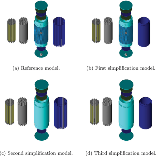
We created the first simplification model, shown in Fig. 1b, by homogenizing the absorber rods to two large circular absorber tubes. For the second simplification model shown in Fig. 1c, we removed the trunnions from the reference model and closed their recesses. Additionally, the cooling fins surrounding the cask were removed.

The third and most simplified model, shown in Fig. 1d, is the combination of the simplifications of the first and the second simplification models; its cooling fins and trunnions are removed, the recesses for the trunnions are closed, and the absorber rods are again homogenized to circular absorber tubes.

We used material descriptions from Ref. [6] for the simulations, and assumed 18×18-24 PWR fuel assemblies, with 300 fuel rods and 24 guide tubes assembled in a square. All fuel rods consist of light water reactor–typical UO₂ fuel with a density of 10.97 g/cm³ in zirconium alloy cladding. We further assumed the cask loading to be homogeneous. This means that all fuel assemblies are identical.

III. SIMULATION AND DATA ANALYSIS

The simulations were conducted utilizing the GEANT4 simulation toolkit^[9–11] to describe the physical processes, such as electromagnetic, hadronic, and optical interactions, as well as long-lived particles, materials, and elements. It tracks the passage of particles through materials employing Monte Carlo methods. Particles are generated using the provided FTFP_ BERT physics list, which is recommended for applications in high-energy physics. To optimize computational efficiency, only muons and antimuons were considered, with all secondaries being annihilated and not tracked. The geometries constituting the models were constructed within the GEANT4 framework.

In our simulations, we posited the generation of mono-energetic muons with an energy of 4 GeV, which corresponds to the average energy of muons at sea level.^[14] Additionally, we considered only monodirectional muons entering at a constant incident angle of 0, corresponding to the incident direction $\vec{z}=(0,0,-1)$ in Fig. 2. The muons were generated over a surface area of $\mathit{x}=[-125\mathrm{cm},125\mathrm{cm}]$ and $\mathit{y}=[-125\mathrm{cm},125\mathrm{cm}]$ at a height of $\mathit{z}=620\mathrm{cm}$ (see Fig. 2).

Fig. 2. Depiction of the orientation of the cask models in the x-, y-, and z-directions relative to the detector plates.

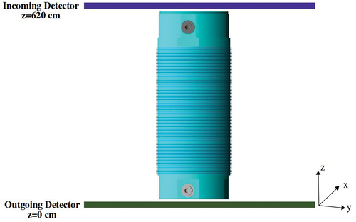
For each simulation, we generated either 4.5 million or 15 million particles. The muons were produced just above the incoming detector, and their incident properties were tracked and stored. Subsequently, they traversed the models, which were positioned perpendicular to the x- and y-planes of the detectors. Thus, the symmetry axis of the models aligned with the z-axis in Fig. 2.

After passing through the geometry, their properties were once again tracked and stored by the outgoing detector. The detectors themselves were considered ideal detectors with dimensions of (500 cm × 500 cm × 1 nm) at positions $z_{\mathrm{inDet}}=(0,0,620,\mathrm{cm})$ and $z_{\mathrm{outDet}}=(0,0,0)$. The tracked properties relevant for data analysis included the incoming and outgoing positions, directions, and particle identifiers (IDs). The latter was crucial to ensuring only muons and antimuons were included in the analysis. The effective scattering angle was obtained by applying Eq. (3)(3) ${\theta }_{\mathrm{eff}}=arccos\left(\frac{\mathit{di}{\mathit{r}}_{\mathit{in}}\cdot \mathit{di}{r}_{\mathit{out}}}{||\mathit{di}{r}_{\mathit{in}}||\cdot ||\mathit{di}{r}_{\mathit{out}}||}\right)\cdot \frac{180}{\pi }$(3) ,

(3) ${\theta }_{\mathrm{eff}}=arccos\left(\frac{\mathit{di}{\mathit{r}}_{\mathit{in}}\cdot \mathit{di}{r}_{\mathit{out}}}{||\mathit{di}{r}_{\mathit{in}}||\cdot ||\mathit{di}{r}_{\mathit{out}}||}\right)\cdot \frac{180}{\pi }$(3)

By using the incoming $\text{Vec}\mathit{di}{r}_{\mathit{in}}$ and outgoing $\text{Vec}\mathit{di}{r}_{\mathit{out}}$ directional information of the particles, this equation allows the calculation of the effective scattering angle for each muon that successfully passes through both detectors. All data were stored in a ROOT file, which was subsequently analyzed using PyROOT within a Jupyter Notebook.

IV. STATISTICAL ANALYSIS

Our data analysis approach involved dividing the data into pixels. For that purpose, Jupyter Notebooks,^[12] with the usage of NumPy,^[15] SciPy,^[16] Astropy,^[17] and Pandas data frames, was used. In detail, we utilized a function that maps incoming continuous position data to integer values representing the ID of the corresponding pixel. The aim was to convert continuous data into discrete units and efficiently process pixelated information for further analysis. The resulting integers were confined to a range of pixel values based on a grid offset of zero and a spacing of 1.5. The pixels ranged from $\mathit{x}=[-125\mathrm{cm},125\mathrm{cm}]$ and $\mathit{y}=[-125\mathrm{cm},125\mathrm{cm}]$, which responds to the particle generation surface. Each pixel contained scatter information, allowing us to create scatter images to visualize and verify the simulation.

In this work, we were interested in the changes of the scattering angle, specifically in the region of the fuel assemblies. Since the surrounding materials affect the scattering angles, we generated difference images to isolate the effects of the fuel assemblies on the muons. To do this, we subtracted the scattering data of the models with fuel assemblies from the scattering data of the same models without fuel assemblies. We conducted a statistical analysis on each pixel data set, wherein we computed the median of the scattering angles. Subsequently, this median value was subtracted from the corresponding pixel in the data set without fuel assemblies. This way, we could analyze the difference in scattering due to the fuel assemblies alone.

The scatter images from simulations with and without fuel assemblies, along with the difference scatter images, are shown in Fig. 3. The order of the four rows represents, from top to bottom, the pixelwise median scattering angles for the reference model and the three simplified models. Each row contains three images. The first column displays the scattering images for the loaded cask model, while the second column presents the results for the empty models. The images were generated through simulation of the reference model (first row), as well as the first, second, and third simplification models (rows 2, 3, and 4, respectively) both with (first column) and without fuel assemblies (second column).

Fig. 3. Scattering images for all models with and without fuel assemblies, as well as difference scattering images. The color code represents the mean of the effective scattering angle ${\theta }_{\mathit{eff}}$ distribution (in degrees) for each pixel, with the x- and y-positions indicating the muon position after traversing the incoming detector.

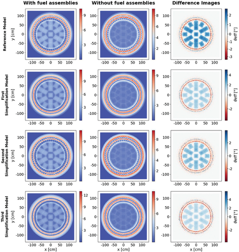
The difference scatter plots in the third column highlight the variations in scattering angles between simulations with and without fuel assemblies. The scattering angles are color coded from blue to red to indicate the corresponding scattering angles. Please be aware that these images serve as visual validation for the model and scattering results (e.g., for symmetry checks). Emphasis on high resolution in the images naturally leads to different scales for the color-coded scattering angles. Consequently, a direct comparison by color alone is not feasible.

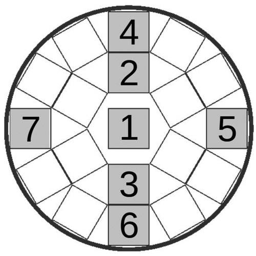
In Fig. 3, the third column showcases the difference images for the corresponding loaded and empty models. The color scheme signifies, for each pixel, the average of the associated effective scattering angle ${\theta }_{\mathrm{eff}}$ distribution (in degrees). The x- and y-positions correspond to the muon position after passing through the incoming detector. For the subsequent statistical analysis, we opted to utilize the difference images. For a thorough examination, we began by choosing pixel IDs linked to the cask region of interest, honing in on specific fuel assemblies marked as 1, 2, 3, 4, 5, 6, and 7 in Fig. 4. Afterward, we extracted the scattering information stored in the pixels corresponding to each fuel assembly area and converted it into a Pandas data frame, generating an individual data frame for every fuel assembly. This procedure was carried out for all simulation data and models.

Fig. 4. Cross-sectional view of the fuel basket, highlighting the fuel assemblies selected for further analysis. These fuel assemblies are labeled with ID numbers 1 through 7 and are color-coded gray for clarity. The fuel assembly had a one-quarter symmetry. Fuel assemblies 5 and 7 were chosen for analysis due to their proximity to the trunnions, while fuel assemblies 4 and 6 were selected for comparison. Fuel assemblies 2 and 3 were chosen for a comprehensive assessment.

Using the resulting data frames, which included the scatter distribution of ${\theta }_{\mathit{eff}}$, a statistical hypothesis test could be performed to determine if there were significant differences in the scatter angles based on the chosen model. To evaluate possible discrepancies in the resulting scattering angles in terms of model accuracy, we used empirical two-sample distribution tests, in particular, the Anderson-Darling test, the Kolmogorov-Smirnov test, and the Kuiper’s test. Utilizing these tests for statistical distribution analysis enabled a comprehensive assessment of the underlying data.

This approach was considered useful for several reasons. First, the Anderson-Darling test, which places more emphasis on the tails of the distribution, is sensitive to subtle differences in extreme values.^[18] In contrast, the Kolmogorov-Smirnov test provides a comprehensive view of differences across the data set,^[19] but especially to variations in the mean.^[20] The Kuiper’s test, on the other hand, is more sensitive to changes in the variance.^[20] Together, these tests provide complementary information that allows for a more holistic understanding of how the data deviate from a theoretical distribution, and they reduce the risk of type I and type II errors by providing a mechanism for cross verification. If all tests consistently reject the null hypothesis, this strengthens the evidence against the hypothesized distribution.

This approach is consistent with standard statistical practice, where the use of multiple tests is recommended to increase the robustness of the results. Overall, the use of the Anderson-Darling test, the Kolmogorov-Smirnov test, and the Kuiper’s test increases the reliability of inferences drawn from the data. These tests calculate the cumulative distribution functions of the scattering angles from each data frame and are explained in detail in the following subsections.

IV.A. Anderson-Darling Test

The quadratic empirical distribution Anderson-Darling test^[21] calculates the cumulative distribution functions of the scattering angles from each data frame. The resulting functions are defined as $F_{{\mathit{n}}_{\mathrm{ref}}}(\mathit{x})$ for the reference model and $F_{m_1}(\mathit{x})$, $F_{m_2}(\mathit{x})$, and $F_{m_3}(\mathit{x})$ for the first, second, and third simplification model, respectively. We than compared and analyzed the data of the reference model with each of the simplification models.

Consider two sample sizes $n_{\mathrm{ref}}$ and $m_{\mathrm{i}}$ of the observations $X_{1_{\mathrm{ref}}}<...<X_{{\mathit{n}}_{\mathrm{ref}}}$ and $Y_{1_{\mathrm{i}}}<...<Y_{{\mathit{m}}_{\mathrm{i}}}$, where i corresponds to the first, the second, and the third simplification models with $\mathrm{i}\in \{1,2,3\}$. $X_{1_{\text{ref}}},..,X_{{\mathit{n}}_{\text{ref}}}$ and $Y_{1_{\text{i}}},..,Y_{{\mathit{m}}_{\text{i}}}$ are pooled and represented by $Z_1,...,Z_{{\mathit{n}}_{\text{ref}}+m_{\text{i}}}$ All values are sorted in ascending order. The statistic is defined as follows^[21]:

(4) $\begin{array}{rl}& A_{{\mathit{n}}_{\mathrm{ref}},m_{\mathrm{i}}}^2=\frac{{\mathit{n}}_{\mathrm{ref}}{m}_{\mathrm{i}}}{n_{\mathrm{ref}}+m_{\mathrm{i}}}\int \frac{{({\mathit{F}}_{{\mathit{n}}_{\mathrm{ref}}}(\mathit{x})-F_{{\mathit{m}}_{\mathrm{i}}}(\mathit{x}))}^2}{H_{{\mathit{n}}_{\mathrm{ref}}+m_{\mathrm{i}}}(\mathit{x})(1-H_{{\mathit{n}}_{\mathrm{ref}}+m_{\mathrm{i}}}(\mathit{x}))}\\ & \mathit{d}{H}_{{\mathit{n}}_{\mathrm{ref}},m_{\mathrm{i}}}(\mathit{x}),& (4)\end{array}$(4)

where $H_{{\mathit{n}}_{\mathrm{ref}}+m_{\mathrm{i}}}$ is defined as the cumulative distribution function of $Z_{{\mathit{n}}_{\mathrm{ref}}+m_{\mathrm{i}}}$,

(5) $H_{{\mathit{n}}_{\mathrm{ref}}+m_{\mathrm{i}}}=\{n_{\mathrm{ref}}{F}_{{\mathit{n}}_{\mathrm{ref}}}(\mathit{x})+m_{\mathrm{i}}{F}_{{\mathit{m}}_{\mathrm{i}}}\}/(n_{\mathrm{ref}}+m_{\mathrm{i}}).$(5)

Equation (4)(4) $\begin{array}{rl}& A_{{\mathit{n}}_{\mathrm{ref}},m_{\mathrm{i}}}^2=\frac{{\mathit{n}}_{\mathrm{ref}}{m}_{\mathrm{i}}}{n_{\mathrm{ref}}+m_{\mathrm{i}}}\int \frac{{({\mathit{F}}_{{\mathit{n}}_{\mathrm{ref}}}(\mathit{x})-F_{{\mathit{m}}_{\mathrm{i}}}(\mathit{x}))}^2}{H_{{\mathit{n}}_{\mathrm{ref}}+m_{\mathrm{i}}}(\mathit{x})(1-H_{{\mathit{n}}_{\mathrm{ref}}+m_{\mathrm{i}}}(\mathit{x}))}\\ & \mathit{d}{H}_{{\mathit{n}}_{\mathrm{ref}},m_{\mathrm{i}}}(\mathit{x}),& (4)\end{array}$(4) uses the weighted quadratic distance between the two cumulative distribution functions $F_{{\mathit{n}}_{\mathrm{ref}}}(\mathit{x})$ and $F_{{\mathit{m}}_{\mathrm{i}}}(\mathit{x})$.^[22] The test statistic can be transformed to

(6) $\begin{array}{rl}& A_{{\mathit{n}}_{\mathrm{ref}},m_{\mathrm{i}}}^2=\frac{{\mathit{n}}_{\mathrm{ref}}{m}_{\mathrm{i}}}{{({\mathit{n}}_{\mathrm{ref}}+m_{\mathrm{i}})}^2}\sum _{\mathit{k}=1}^{{\mathit{n}}_{\mathrm{ref}}+m_{\mathrm{i}}}\\ & \frac{{({\mathit{F}}_{{\mathit{n}}_{\mathrm{ref}}}(Z_k)-F_{{\mathit{m}}_{\mathrm{i}}}(Z_k))}^2}{H_{{\mathit{n}}_{\mathrm{ref}}+m_{\mathrm{i}}}(Z_k)(1-H_{{\mathit{n}}_{\mathrm{ref}}+m_{\mathrm{i}}}(Z_k))}.& (6)\end{array}$(6)

IV.B. Kolmogorov-Smirnov Test

Conversely, the two-sample Kolmogorov-Smirnov test computes the supremum distance between the respective empirical distribution functions, also denoted as $F_{{\mathit{n}}_{\mathrm{ref}}}(\mathit{x})$ and $F_{m_1}(\mathit{x})$, $F_{m_2}(\mathit{x})$, and $F_{m_3}(\mathit{x})$, using the two sets of samples $X_{1_{\mathrm{ref}}},..,X_{{\mathit{n}}_{\mathrm{ref}}}$ and $Y_{1_{\mathrm{i}}},..,Y_{{\mathit{m}}_{\mathrm{i}}}$.^[19] The test statistic generalizes to

(7) $\mathit{K}{S}_{{\mathit{n}}_{\mathrm{ref}}{m}_{\mathrm{i}}}=\sqrt{\frac{{\mathit{n}}_{\mathrm{ref}}{m}_{\mathrm{i}}}{n_{\mathrm{ref}}+m_{\mathrm{i}}}}\mathrm{su}{\mathrm{p}}_x|F_{{\mathit{n}}_{\mathrm{ref}}}(\mathit{x}))-F_{{\mathit{m}}_{\mathrm{i}}}(\mathit{x})|.$(7)

The two empirical distribution functions $F_{{\mathit{n}}_{\mathrm{ref}}}(\mathit{x})$ and $F_{{\mathit{m}}_{\mathrm{i}}}(\mathit{x})$ are based on the sample sizes $n_{\mathrm{ref}}$ and $m_{\mathrm{i}}$, respectively.^[19] The null hypothesis claims that the samples $X_1,...,X_n$ and $Y_1,...,Y_m$ are drawn from the same distribution and is rejected if $\mathit{K}{S}_{{\mathit{n}}_{\mathrm{ref}}{m}_{\mathrm{i}}}$ is larger than a certain critical value $\mathit{K}{S}_{\alpha }$ for a given significance level $\mathit{\alpha }$.^[23] $\mathit{K}{S}_{\alpha }$ can be calculated using the following equation:

(8) $\mathit{K}{S}_{\alpha }=\sqrt{-\frac{1}{2}\cdot \ln \left(\frac{\alpha }{2}\right)}\sqrt{\frac{{\mathit{n}}_{\mathrm{ref}}+m_{\mathrm{i}}}{n_{\mathrm{ref}}\cdot m_{\mathrm{i}}}}.$(8)

In our analysis, we make use of the p-value in the case of the Kolmogorov-Smirnov test. It is derived through a calculation based on the test statistic and the sample sizes. Refer to Ref. [24] for further details.

IV.C. Kuiper’s Test

As a third test, we included the Kuiper’s test^[25] in our analysis. We assumed again that we have the distributions $X_{1_{\mathrm{ref}}},..,X_{{\mathit{n}}_{\mathrm{ref}}}$ and $Y_{1_{\mathrm{i}}},..,Y_{{\mathit{m}}_{\mathrm{i}}}$ with cumulative distribution functions $F_{{\mathit{n}}_{\mathrm{ref}}}(\mathit{x})$ and $F_{{\mathit{m}}_{\mathrm{i}}}(\mathit{x})$ with $\mathrm{i}\in \{1,2,3\}$. The Kuiper’s test is an extended version of the Kolmogorov-Smirnov test. It is different from the Kolmogorov-Smirnov test [compare to Eq. (7)(7) $\mathit{K}{S}_{{\mathit{n}}_{\mathrm{ref}}{m}_{\mathrm{i}}}=\sqrt{\frac{{\mathit{n}}_{\mathrm{ref}}{m}_{\mathrm{i}}}{n_{\mathrm{ref}}+m_{\mathrm{i}}}}\mathrm{su}{\mathrm{p}}_x|F_{{\mathit{n}}_{\mathrm{ref}}}(\mathit{x}))-F_{{\mathit{m}}_{\mathrm{i}}}(\mathit{x})|.$(7) ] in that it uses the sum of the positive and negative maximum distance of $F_{{\mathit{n}}_{\mathrm{ref}}}(\mathit{x})$ and $F_{{\mathit{m}}_{\mathrm{i}}}(\mathit{x})$.^[20] The Kuiper’s test is more effective at detecting changes in variance compared to changes in the mean, which is a strength it has over the Kolmogorov-Smirnov test,^[20]

(9) $\begin{array}{rl}& \mathit{K}{U}_{{\mathit{n}}_{\mathrm{ref}}{m}_{\mathrm{i}}}=\sqrt{\frac{{\mathit{n}}_{\mathrm{ref}}{m}_{\mathrm{i}}}{n_{\mathrm{ref}}+m_{\mathrm{i}}}}\left[\mathrm{su}{\mathrm{p}}_x(F_{{\mathit{n}}_{\mathrm{ref}}}(\mathit{x}))-F_{{\mathit{m}}_{\mathrm{i}}}(\mathit{x}))\right.\\ & \left.+\mathrm{su}{\mathrm{p}}_x(F_{{\mathit{m}}_{\mathrm{i}}}(\mathit{x})+F_{{\mathit{n}}_{\mathrm{ref}}}(\mathit{x}))\right].& (9)\end{array}$(9)

In the analysis, we followed the same strategy as for the Kolmogorov-Smirnov test and used the p-value to assess the validity of the null hypothesis. For further details, please see Ref. [17].

All calculation steps explained in Secs. IV.A and IV.B were calculated using the SciPy packages the Anderson-Darling test for k-samples and the two-sample Kolmogorov-Smirnov test. For the former, it returns the normalized two-sample Anderson-Darling test statistic and the p-values, as well as the critical values for each level of significance. For the latter, it returns the Kolmogorov-Smirnov test statistic and the p-value. For the calculations in Sec. IV.C, we used the Astropy package kuiper_two. This package calculates the raw Kuiper test statistic as well as the p-value of the two distributions to be compared.

Depending on the output of the tests, we decided whether we assumed, depending on a pre-set level of significance, that the two samples were from the same or a different distribution. We defined a null hypothesis $H_0$ that states that the analyzed data were drawn from same distribution.

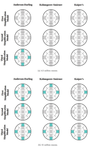
In the case of model comparisons, the meaning was defined as follows. If $H_0$ was rejected, it was assumed that the scattering angles were significantly influenced by the model simplifications to our chosen levels of significance of 1%. On the basis of that, we decided whether a model simplification had a significant impact on the scattering angles. An exemplary representation of the difference scattering data stored in the area of fuel assembly 5 (simulation performed with 15 million muons) can be seen in Fig. 6.

V. RESULTS

To analyze the model-dependent variations in scattering angles, we investigated in detail seven representative fuel assemblies (as shown in Fig. 4). They had unique positions within the fuel basket, showing diverse characteristics in realistic loading scenarios. The inclusion of symmetrical fuel assemblies in our analysis served to avoid mistakenly assuming an influence on scattering angles, whether in the inner or outer row, respectively, due to statistical factors. This ensured a more accurate assessment of the model-dependent effects.

The first assembly was positioned at the center of the cask, and for a homogeneous loading, it would be the hottest due to dissipation of decay heat in the cask. The remaining assemblies were positioned in two concentric circles around the central one. Additional to the central fuel assembly, we further chose six assemblies, two from the inner ring and four from the outer ring, as shown in Fig. 4. On the outer ring, fuel assemblies 5 and 7 were located next to the trunnions. Any effect the latter had would be visible by comparing the scattering angles of fuel assemblies 5 and 7 with 4 and 6, respectively. We compared the scattering angle distributions for the different modeling assumptions and sample sizes.

Using the Anderson-Darling and Kolmogorov-Smirnov tests, we analyzed the respective difference data sets. The critical value ${A_c}^2$ for the Anderson-Darling test for a level of significance of 1% was ${A_c}^2$ = 3.752. If the resulting test statistic $A_{{\mathit{n}}_{\mathrm{ref}},m_{\mathrm{i}}}^2$ was smaller than the critical value, we did not reject the null hypothesis $H_0$ to a level of significance of 1%. If the value was larger, we rejected it. For the Kolmogorov-Smirnov and the Kuiper’s tests, we made use of the p-value. In the context of statistical distribution tests, if a p-value was smaller than a specific predetermined significance level $\mathit{\alpha }$, it indicated the statistical incompatibility of the data. In our case, if $\mathit{\alpha }=0.01>\mathit{p}$, we rejected the null hypothesis.

In Fig. 5, the difference data of the reference model were compared to all difference data of the simplification models. If a fuel assembly is color-coded turquoise, the null hypothesis was rejected. The figure shows the results for each statistical distribution test and particle number. The accordingly calculated test statistic for the Anderson-Darling test and the calculated p-values for the Kolmogorov-Smirnov and Kuiper’s tests can be found in Table III.

TABLE III Calculated Test Statistics for the Anderson-Darling Test and the Calculated p-Value for the Kolmogorov-Smirnov and Kuiper’s Tests After Comparison Between the Reference Model and All Simplified Models*

	ID	Anderson-Darling		Kolmogorov-Smirnov		Kuiper’s Test
Number of muons		4.5 × 10^6	15 × 10^6	4.5 × 10^6	15 × 10^6	4.5 × 10^6	15 × 10^6
Reference versus	1	−0.44005	−0.47863	0.77235	0.42468	0.57763	0.92316
simplified model 1	2	−0.64648	−0.02685	0.88048	0.44341	0.91303	0.08630
	3	−0.64944	0.03012	0.94116	0.58468	0.97497	0.65694
	4	0.44497	5.02497	0.31281	0.00964	0.82401	0.02131
	5	1.96998	7.47372	0.15056	0.00027	0.19996	0.00896
	6	0.75842	3.34086	0.18695	0.01066	0.18328	0.20213
	7	0.61845	6.35889	0.20115	0.00200	0.68386	0.01048
Reference versus	1	−0.41614	−0.78526	0.26775	0.73489	0.77667	0.38569
simplified model 2	2	−0.78383	−0.82529	0.95828	0.80412	0.82780	0.98605
	3	−0.76802	−0.81225	0.71804	0.91882	0.78876	0.61051
	4	−0.84654	0.8453	0.73727	0.31954	0.44890	0.21850
	5	−0.38159	1.76414	0.72196	0.14144	0.14010	0.54692
	6	0.22059	0.15172	0.58521	0.44156	0.29952	0.41748
	7	0.12956	1.47785	0.05910	0.12367	0.87213	0.36858
Reference versus	1	−0.92746	−0.89796	0.67472	0.88712	0.43205	0.57559
simplified model 3	2	−0.51529	−0.02316	0.87405	0.49242	0.74126	0.43538
	3	−0.54906	0.06878	0.84193	0.71632	0.87818	0.71944
	4	1.42972	10.70780	0.06391	0.00073	0.57374	0.01572
	5	4.47591	16.87124	7.86835E-25	0.00001	0.01285	0.00062
	6	4.04571	7.46859	0.09898	0.00659	0.0516	0.00034
	7	2.84604	14.82826	0.03102	0.00003	0.23082	0.00004

*Results for both particle numbers are listed.

Fig. 5. Illustration of the rejection of the null hypothesis after comparing the difference data of the simplified models to the simplified models. The fuel assembly regions are colored turquoise if the data sets with the scattering angles contained therein led to a rejection of the null hypothesis. The results for all three tests for simulations performed with 4.5 million and 15 million muons are shown in (a) and (b), respectively.

VI. DISCUSSION

Our analysis showed that taking a level of significance of 1% and the particle number of 4.5 million muons, the null hypothesis could not be rejected for any model applying the Kolmogorov-Smirnov test or the Kuiper’s test. However, when employing the Anderson-Darling test and specifically comparing the reference model with the third simplification model, it was evident that all the outer fuel assemblies were significantly influenced by the simplifications due to the rejection of the null hypothesis.

With a particle number of 15 million resulting in larger sample sizes, all tests exhibited different outcomes compared to the smaller samples. The Kolmogorov-Smirnov test indicated significant influence on three out of four outer fuel assemblies when comparing the reference model to the first simplification model. Conversely, the Kuiper’s test identified an influence on one out of four outer fuel assemblies in this scenario. When comparing to the third simplification model, the Kolmogorov-Smirnov test rejected the null hypothesis for all four outer fuel assemblies. The Kuiper’s test rejected the null hypothesis $H_0$ in three out of four cases concerning the outer fuel assemblies.

In contrast, the Anderson-Darling test yielded different results. It rejected the null hypothesis for all outer fuel assemblies when comparing the reference model to both the first and third simplification models. However, for the comparison to the second simplification model, $H_0$ was only rejected for three out of four assemblies. In total there were four fuel assemblies that were rejected equally by all three tests.

Figure 6 shows the probability as well as the cumulative function for data stored in fuel assembly 6. The simulations were performed with 15 million and the comparison for all models is shown. Comparing the results shown in Fig. 5b, we observed a rejection of the null hypothesis in two out of three scenarios ($H_0$ rejected by all three tests). By analyzing the extreme values within the cumulative distribution functions of the reference model and the simplified models, the test outcome could be explained, especially in the case of the Anderson-Darling test. The rejection of the null hypothesis occurred due to the test’s particular sensitivity to disparities in extreme values, particularly in the tails of the distribution. Consequently, through a thorough comparison of the three cumulative distribution functions and their extreme values in Fig. 6, the Anderson-Darling test rejected the null hypothesis of data sets where differences in extreme values were pronounced, more precisely in Figs. 6b and 6c.

Fig. 6. (left) Comparison of the probability distribution function and (right) the cumulative probability function of the reference model (black) with the simplified models (red) of scatter data stored in the pixels representing fuel assembly 5 generated using 15 million muons.

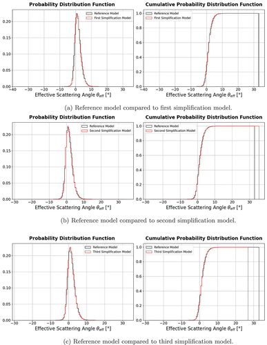
Although the maximum values in Fig. 6a were closely aligned, a quick examination of the two data sets revealed significant disparities among their top 10 largest values, leading to differences in the tails. In contrast, the Kolmogorov-Smirnov test examined the differences in the entirety of the data sets. Hence, the interpretation of the results proved to be more complicated and could not be done only by visually examining the cumulative distribution functions. The same applied to the Kuiper’s test. A closer look at the four statistical moments (especially the mean and the variance) would be necessary to make a sound statement about the behavior of both tests, but that is beyond the scope of this paper.

The analysis additionally showed that when discerning variations in the scattering distribution, small sample sizes, such as those generated with simulations using 4.5 million muons, may prove insufficient for a comprehensive analysis. Significant influences were found in some cases (see Table III, specifically, 4.5 million muons, Anderson-Darling test, comparison between reference model and third simplification model), but by using 15 million muons, the percentage of fuel assemblies that experienced a significant impact increased in both the Anderson-Darling and Kolmogorov-Smirnov tests. Using the Anderson-Darling test, an increase of about 52% was observed, while the Kolmogorov-Smirnov test showed an increase of 33%. The Kuiper’s test rejected the null hypothesis with a percentage of 19.

If only the outer fuel assemblies were considered, 22/36 (11 with the Anderson-Darling test, 7 with the Kolmogorov-Smirnov test, and 4 with the Kuiper’s test) experienced significant influence using 15 million particles. In the case of 4.5 million, only 4/24 (all four with the Anderson-Darling test) experienced significant influence. It is clear that outliers can occasionally occur in the data set and are reflected in the tails of the distributions. Given the sensitivity of the Anderson-Darling test to differences in the tails, we chose to reject the null hypothesis only if all three tests rejected it for the specific fuel assembly.

Finally, we would like to emphasize that the cask geometry was symmetrical, implying that opposite fuel assemblies would be rejected or not rejected to the same extent. If this symmetry is not maintained, it raises questions about whether the statistics will be sufficient. Consequently, simulations with 15 million muons may not yield to a sample size large enough for an overall reliable analysis for all three tests.

VII. CONCLUSION AND OUTLOOK

In conclusion, this study highlighted the impact of simplifying the Castor cask model for muon scattering angle simulations, particularly for fuel assemblies in proximity to these simplifications. Therefore, a careful assessment of the model’s degree of simplification was required to ensure the precision and reliability of the results. Given the specific requirements and objectives of muon radiography on spent fuel casks, our findings underscore the essential need for an accurate model to obtain trustworthy scattering data. Even minor simplifications, such as omitting trunnions and homogenizing the polyethylene rods, can have a noteworthy effect.

Depending on the analysis objective, such as achieving single-rod resolution, the chosen modeling approach can significantly shape the results. For instance, comparing the reference model with the third simplification model requires acknowledgment that simplifying the polyethylene rods to two large tubes and excluding trunnions impacts the scatter distribution in the fuel assemblies of the outer ring. The rejection of the null hypothesis $H_0$ for the investigated outer fuel assemblies in all three tests reinforced this observation (rejection of 4/4 for the Anderson-Darling test and the Kolmogorov-Smirnov test and 3/3 for the Kuiper’s test, respectively).

Our analysis further demonstrated that modeling simplifications did not yield a statistically significant impact on the inner fuel assemblies 1, 2, and 3 for both sample sizes.

If a comprehensive analysis of all fuel assemblies in the cask is desired, our findings indicated that modeling simplifications, as seen in the first and third models, could result in statistically significant differences in muon scattering angle distributions. However, in the case of the second simplification model, we observed that the simplifications (neglecting cooling fins and trunnions) had no statistical influence on the muon scattering distribution. It can be inferred that simplifying or omitting geometries, such as trunnions and cooling fins at the edge of the cask, has negligible impact on the effective scattering angles of muons within the fuel assembly region However, the transformation of polyethylene rods into tubes (Figs. 6a and 6c) demonstrated a significant influence on the resulting angles. Whether this effect was due to the proximity to the fuel assembly or to the specific geometric simplification requires further investigation and detailed analysis.

In this analysis, we presented results for entire fuel assemblies by aggregating information at the corresponding pixel level. However, the segmentation of the cask’s axial slice into pixels opens up the possibility of investigating smaller geometric entities, such as rows of fuel rods or individual fuel rods.

Future work aims to incorporate a more realistic muon spectrum, akin to that provided by Ref. [26]. This entails considering muons with a broader range of energies and incidence angles, potentially resulting in a greater number of signals within the same experimental period. To maintain comparable resolution of the difference images outlined in this study, a selection of signals based on angles becomes crucial.

Acknowledgments

We would like to thank Nadine Berner, Germano Bonomi, Paolo Checchia, Altea Lorenzon, and Marc Péridis for valuable comments and discussions.

Disclosure Statement

No potential conflict of interest was reported by the authors.

Notes

^a For simplicity, we refer to this as Castor in this paper.

References

- K. N. BOROZDIN et al., “Radiographic Imaging with Cosmic-Ray Muons,” Nature, 422, 6929, 277 (2003); https://doi.org/10.1038/422277a.
- G. BONOMI et al., “Applications of Cosmic-Ray Muons,” Prog. Part. Nucl. Phys., 112, 103768 (2020); https://doi.org/10.1016/j.ppnp.2020.103768.
- G. R. LYNCH and O. I. DAHL, “Approximations to Multiple Coulomb Scattering,” Nucl. Instrum. Methods Phys. Res. Sect. B, 58, 1, 6 (1991); https://doi.org/10.1016/0168-583X(91)95671-Y.
- T. M. KNASEL, “Accurate Calculation of Radiation Lengths,” Nucl. Instrum. Methods, 83, 2, 217 (1970); https://doi.org/10.1016/0029-554X(70)90461-1.
- R. L. WORKMAN et al., “Review of Particle Physics,” Prog. Theor. Exp. Phys., 2022, 8, 083C01 (2022); https://doi.org/10.1093/ptep/ptac097.
- “Product Info Castor V/19,” Gesellschaft fur Nuklear-Service; https://www.gns.de/language=en/21551/castor-v-19.
- T. BRAUNROTH et al., “Muon Radiography to Visualise Individual Fuel Rods in Sealed Casks,” EPJ Nucl. Sci. Technol., 7, 12, 12 (2021); https://doi.org/10.1051/epjn/2021010.
- A. GEORGADZE, “Fast Verification of Spent Nuclear Fuel Dry Casks Using Cosmic Ray Muons: Monte Carlo Simulation Study,” Physics, arXiv:2112.03274 (2021); https://doi.org/10.48550/arXiv.2112.03274.
- S. AGOSTINELLI et al., “Geant4—a Simulation Toolkit,” Nucl. Instrum. Methods Phys. Res. Sect. A, 506, 3, 250 (2003); https://doi.org/10.1016/S0168-9002(03)01368-8.
- J. ALLISON et al., “Geant4 Developments and Applications,” IEEE Trans. Nucl. Sci., 53, 1, 270 (2006); https://doi.org/10.1109/TNS.2006.869826.
- J. ALLISON et al., “Recent Developments in Geant4,” Nucl. Instrum. Methods Phys. Res. Sect. A, 835, 186 (2016); https://doi.org/10.1016/j.nima.2016.06.125.
- T. KLUYVER et al., “Jupyter Notebooks—A Publishing Format for Reproducible Computational Workflows,” presented at the Int. Conf. on Electronic Publishing (2016).
- J. NIEDERMEIER and M. STUKE, “Impact of Modeling Assumptions on Muon Scattering Images of Loaded Dry Storage Casks,” presented at the Int. Conf. on Mathematics and Computational Methods Applied to Nuclear Science and Engineering (2023).
- J. AUTRAN et al., “Characterization of Atmospheric Muons at Sea Level Using a Cosmic Ray Telescope,” Nucl. Instrum. Methods Phys. Res. Sect. A, 903, 77, 77 (2018); https://doi.org/10.1016/j.nima.2018.06.038.
- C. R. HARRIS et al., “Array Programming with NumPy,” Nature, 585, 7825, 357 (2020); https://doi.org/10.1038/s41586-020-2649-2.
- P. VIRTANEN et al., “SciPy 1.0: Fundamental Algorithms for Scientific Computing in Python,” Nat. Methods, 17, 3, 261 (2020); https://doi.org/10.1038/s41592-019-0686-2.
- ASTROPY COLLABORATION et al. “The Astropy Project: Sustaining and Growing a Community-Oriented Open-Source Project and the Latest Major Release (v5.0) of the Core Package,” J. Astronomical, 935, 2, 167(2022); https://doi.org/10.3847/1538-4357/ac7c74.
- F. W. SCHOLZ and M. A. STEPHENS, “K-Sample Anderson-Darling Tests,” J. Am. Stat. Assoc., 82, 399, 918 (1987); https://doi.org/10.2307/2288805.
- S. ENGMANN and D. COUSINEAU, “Comparing Distributions: The Two-Sample Anderson–Darling Test as an Alternative to the Kolmogorov–Smirnov Test,” J. App. Quant. Methods, 6, 1, (2011).
- M. A. STEPHENS, “Use of the Kolmogorov-Smirnov, Cramer-Von Mises and Related Statistics Without Extensive Tables,” J. R. Stat. Soc. Series B (Methodol.), 32, 1, 115 (1970); https://doi.org/10.1111/j.2517-6161.1970.tb00821.x.
- T. W. ANDERSON and D. A. DARLING, “A Test of Goodness of Fit,” J. Am. Stat. Assoc., 49, 268, 765 (1954); http://www.jstor.org/stable/2281537.
- A. N. PETTITT, “A Two-Sample Anderson-Darling Rank Statistic,” Biometrika, 63, 1, 161 (1976); https://doi.org/10.2307/2335097.
- D. A. DARLING, “The Kolmogorov-Smirnov, Cramer-von Mises Tests,” Ann. Math. Statist., 28, 4, 823 (1957); https://doi.org/10.1214/aoms/1177706788.
- E. JONES et al., “SciPy: Open Source Scientific Tools for Python,” SciPy (2001). http://www.scipy.org/.
- N. H. KUIPER, “Tests Concerning Random Points on a Circle,” Nederl. Akad. Wetensch. Proc. Ser. A, 63, 38 (1960); https://doi.org/10.1016/S1385-7258(60)50006-0.
- D. PAGANO et al., “EcoMug: An Efficient COsmic MUon Generator for Cosmic-Ray Muon Applications,” Nucl. Instrum. Methods Phys. Res. Sect. A, 1014, 165732 (2021); https://doi.org/10.1016/j.nima.2021.165732.