Securing Anomaly Detection for Process-Based Time Series

Abstract

Widespread innovation from artificial intelligence and machine learning (AI/ML) tools presents a lucrative opportunity for the nuclear industry to improve state-of-the-art analyses (e.g. condition monitoring, remote operation, etc.) due to increased data visibility. In recent years, the risk posed by collaborative data exchange has received increased attention due, in part, to a potential adversary’s ability to reverse-engineer intercepted data using domain knowledge and AI/ML tools. While the efficacy of typical encryption has been proven during passive communication and data storage, collaborative exchange typically requires decryption for extended analyses by a third-party, which poses an intrinsic risk due to these trustworthiness concerns. The directed infusion of data (DIOD)¹

¹ A.Al Rashdan and H.Abdel-Khalik, Deceptive Infusion of Data, Non-Provisional Patent, Application No. 63/227,389, September 2022.

paradigm presented in this paper discusses a novel data masking technique that relies on preserving the usable information of proprietary data while concealing its identity via reduced-order modeling. In contrast to existing state-of-the-art data masking methods, DIOD does not impose limiting assumptions, computational overheads, or induced uncertainties, thereby allowing for secure and flexible data-level security that does not alter the inferential content of the data. This paper focuses on the application of DIOD to a process-based simulation wherein a leaking reservoir with a controlled inlet pump is simulated under various experimental conditions with the goal of producing masked data that preserve the information given by anomalies. These experiments included the injection of statistically significant anomalies, subtle anomalies that occurred over an extended period, and the addition of several independent anomalous states. Each experiment showed that a classifier will identify the same anomalies whether it analyzes the original or masked data. An additional experiment also tested the case of corrupted labeling information wherein labels were arbitrarily randomized, and the loss in labeling accuracy was about the same for both datasets. Each of these experiments show that data obfuscated by DIOD may be utilized in the place of real data for a variety of condition monitoring scenarios with no loss in performance.

Keywords:

• Machine learning
• data privacy
• time series
• secure collaboration
• inference-preserving data masking

I. INTRODUCTION

The nuclear industry has seen a drastic rise in the volume of usable data due to the recent deployment of artificial intelligence and machine learning (AI/ML) capabilities and the rise of active monitoring protocols. The large volume of data recovered by these tools, if properly utilized, can facilitate procedures such as condition monitoring and autonomous control schemes, thereby enabling safe, efficient, and cost-effective operation of nuclear plants. Continued integration of these tools is crucial to extending the operation of existing nuclear reactor technologies, such as large-scale boiling-water reactors and pressurized-water reactors. Autonomous control and AI/ML tools are also crucial for the development of next-generation mixed-source power systems, such as the study of IoT-based hybrid energy systems, an economic analysis of co-generation plants, and the development of advanced / modularized designs.^[1,2]

While they often aid in streamlining engineering analytics, AI/ML tools are complex and may require vast data preprocessing, hyperparameter tuning, and comparative benchmarking, which often warrant collaborative exchange between data holders (e.g., teams associated with the research and development goals of a nuclear power company) and various analyst firms that specialize in technological development (e.g., researchers from academia or vendors). As the volume, variety, and complexity of data expand, so do the barriers to entry for in-house data analytics, thus rendering collaboration an attractive investment to properly assess and compare proprietary AI/ML tools.

Among the primary challenges faced by the nuclear industry is the sensitive nature of its data which may involve proprietary systems or invoke national security concerns due to its proximity to restricted procedures. Data leakage, which has become a major concern in recent years, presents an inherent risk due to the potential loss of proprietary information.^[3] Many sources focus on a network-level risk assessment and protection of the so-called critical digital assets within the nuclear industry.^[4,5] However, data details such as core design or fuel composition may present an inherent risk to information security if they can be reverse-engineered using domain-specific knowledge. Complex analyses such as condition monitoring may require an intrusive AI/ML-based approach since they often entail large volumes of data and a specific range of so-called anomalies.^[6] Validation of the resulting model may also require data transfer for comparative benchmarking across similar experiments, systems, or analyses. The high-dimensional time series data used in condition monitoring, however, are quite revealing since they contain information pertaining to the physical conservation laws of the nuclear core that may contain system design details and fuel information. The DIOD methodology presents an efficient data-based solution to mitigate trustworthiness concerns while maintaining the fidelity of engineering analytics.

Data privacy efforts typically focus on the threat posed by the so-called adversary (e.g., a rival business or hacker) at the network level, whose goal is presumed to involve data theft or exploitation. Typical data masking techniques rely on several approaches to obfuscate usable data such that proprietary details cannot be learned, used, or uncovered by the adversary; the obfuscated data are usually referred to as masked data. In terms of data transfer, the adversarial threat is often seen as the potential for a third party to intercept (or otherwise access) sensitive files. In this case, data protection is often procured by methods such as encryption whose security relies on a highly complex and reversible data obfuscation accessible if, and only if, the analyst is permitted access via the decryption key.^[7–9] Data security in storage or during one-time transfer is well understood in industry. The greater risk, however, is that data exchange for analytic purposes or collaborative endeavors requires the explicit communication of proprietary details with the trusted analyst and any other involved parties. Even though the analyst may be fully trustworthy, the enlarged risk posed by the act of data disclosure across several networks has received increased attention. In a more extreme case, there is a major risk of data leakage posed by a potentially malicious analyst. Both concerns are hereinafter referred to as “the issue of trust,” and several methods have proposed solutions, including homomorphic encryption (HE), differential privacy, and a variety of multiparty computation techniques.^[10–15] Each technique seeks to alleviate the issue of trust by avoiding the need to distribute the original information directly, and each technique uses the masked data directly at some point in its respective procedures. That is, masked data may be used by the analyst in place of the original data.

Among the most popular of the emerging techniques is HE wherein mathematical operations are preserved during decryption by the stakeholder. That is, the data analyst applies some algorithm to the encrypted data and returns it to the stakeholder, who can decrypt it in order to obtain usable results.^[10] While identifying a fully HE (FHE) scheme that is guaranteed to preserve all mathematical operations is very computationally intensive, variations such as Somewhat HE have been proposed as a less demanding variation of the technique. The compromise, however, is that the mathematical capabilities of the analyst are limited in scope or quantity.^[16] While such assumptions can be managed, limitations on the complexity of analyses may prove infeasible to certain applications. Emerging methods may also utilize certain forms of cloud computation alongside HE schemes to strengthen security in an untrustworthy cloud environment.^[17]

Another major family of techniques involves differential privacy, which adds selective levels of noise to provide a corresponding privacy guarantee.^[11,12] The addition of random noise affects the precision of reverse engineering since details cannot be deterministically ascertained by an adversary, thereby providing a mathematical bound on at-risk information. In other words, the amount of information recoverable by an outside party is limited, while the majority of the data’s utility toward downstream analyses is preserved. The inherent trade-off is that newly formed data contain an induced level of uncertainty due to the addition of noise, requiring more data to compensate when training an AI/ML model.^[11–12] As such, industries with a large privacy requirement and limited data, such as the nuclear industry, may suffer from artificially weakened analyses. For instance, process-based data may already contain large noise levels due to background interference and faulty sensor measurements, rendering it impractical to add even more noise. Some extensions mitigate this downside with a careful choice of parameters such as the level and characteristics of additive noise.^[12]

A large variety of multiparty computing (MPC) techniques that may distribute “partial information” to third parties (thereby enabling cooperation on a larger scale) have also received increased attention.^[13,15] Data security is greatly improved since no individual possesses total knowledge of the system or data, aside from the original stakeholder.

To avoid the possibility of data leakage via centralized platforms, many recent techniques make use of so-called federated learning as an alternative to centralized computation wherein privacy is enforced by the fact that local data will not be transferred beyond its original owner.^[14] Instead, each individual owner trains their own model, the collection of which is aggregated downstream. However, results may be limited since the underlying data, and therefore the trained models, may be highly differentiated among various data holders. This has led some authors to use the prior distributions of each model as real-data approximations (without destroying privacy) to apply federated learning.^[14] Similarly, the recent advent of local differential privacy relaxes the assumptions of the standard approach by allowing each stakeholder to apply differential privacy according to their acceptable tolerance, which has distinct advantages for highly differentiated data, such as the current Internet-of-Things market.^[18,19]

Each technique discussed in this section successfully addresses the issue of trust by providing usable masked data, in some form, wherein the analyst(s) is not privy to proprietary details; the potential limitation of each case, however, lies in their limiting assumptions. In HE, the analyst’s ability is diminished, and applying FHE schemes to compensate for this requires vast computational overheads in the current state of the art, which may be infeasible to applications such as real-time analytics and high-dimensional computation. Differential privacy injects artificial uncertainty into the data, thereby weakening high-fidelity data that may already contain process noise. While MPC and/or federated learning address the risk of data privacy and the lack of trust, there is a risk of model bias that is difficult to predict for specialized applications such as nuclear power.

The focus of this paper lies in the extension of a novel data masking paradigm called the directed infusion of data (DIOD) that constructs usable masked datasets while avoiding the various constraints of each method. By utilizing the behavior of a secondary dataset, DIOD’s transformation isolates the usable, information-carrying portion of the original data and associates that subset of information with another system’s behavior and/or visual characteristics. As a brief illustration, suppose that the data contains time series signals from proprietary simulation software. The important artifacts of its behavior, such as correlations between variables or transient effects, can be associated with the visual characteristics of an unrelated dataset, such as a different simulation, stakeholders can freely pass the new dataset without divulging any proprietary details while the data analyst solves an equivalent problem.

A previous publication introduced DIOD from a theoretical perspective and gave a brief classification problem.^[20] A condition monitoring experiment was conducted with the Idaho National Laboratory whose implementation forms the basis of this paper.^[20,21]

The rest of this paper is organized as follows. Sections II and III provide an overview of DIOD in a theoretical sense and an overview of the experimental simulation used throughout this paper, respectively. Section IV conducts an initial condition monitoring experiment using large anomalies, and Sec. V builds on these results shown by applying a subtle condition monitoring experiment. Section VI further extends previous experiments by evaluating a case where several anomalous regimes are considered, and Sec. VII gives a brief discussion on the case of corrupted labeling information within this experimental case. An evaluation of each case (comparing the original and the masked data) is given in Sec. VIII, and concluding remarks are given in Sec. IX.

II. METHODOLOGY

The DIOD methodology takes a similar design philosophy to several techniques discussed in the previous section by directly using masked data rather than relying on any form of decryption. DIOD begins by identifying two independent sets of data. The first dataset is the sensitive data that contain original system information, hereinafter referred to as the proprietary data. The second dataset, which is known hereinafter as the generic data, should be completely unrelated to the proprietary data and underlying system. For example the proprietary data may originate from the sensors of a nuclear power plant, and the generic data may comprise the behavior of a solar array, econometric modeling, the mechanical performance of a car engine, etc. The only requirement for the generic data in this case is that it contain the same number of features. For instance, if the proprietary data measure 100 features across 1000 time steps, then the generic data must also contain 100 features, but the measurement may consider, for example, 10,000 time steps. If the dataset is too large to find an appropriate generic system, then equation-based generic data may be used.

Once identified, the next step of DIOD is to decompose the target data. Though it is a broad topic within engineering communities, data decomposition may be thought of as breaking down the data to form elementary trends so that the data can be easily understood, reduced, and reconstructed. The two datasets are each decomposed via a user-specified reduced-order modeling (ROM) technique (e.g., Fourier-based techniques, principal component analysis, dynamic mode decomposition, etc.) to isolate $\mathit{r}$ components of the so-called inferential metadata that may be utilized to reform the original data. These subsets are denoted as $\mathit{\psi }$ and $\mathit{\varphi }$, respectively, that may be utilized to reform the original data.^[22–24] Briefly, Eqs. (1)(1) $y_P\left(\mathit{x},\mathit{\alpha }\right)\approx \sum _{\mathit{i}=1}^r{\psi }_i^P\left(\mathit{x}\right){\varphi }_i^P\left(\mathit{\alpha }\right)$(1) and (2)(2) $y_G\left(x^{\prime },{\alpha }^{\prime }\right)\approx {\displaystyle \sum _{\mathit{i}=1}^r{\psi }_i^G\left(x^{\prime }\right)}{\varphi }_i^G\left({\alpha }^{\prime }\right)$(2) denote that the proprietary and generic data, respectively, are approximately formed by $\mathit{r}$ summed terms of $\mathit{\psi }$ and $\mathit{\varphi }$ (which is equivalent to a matrix operation), where $\mathit{r}$ is chosen to reconstruct the data to a user-specific error tolerance. Each variable in Eqs. (1)(1) $y_P\left(\mathit{x},\mathit{\alpha }\right)\approx \sum _{\mathit{i}=1}^r{\psi }_i^P\left(\mathit{x}\right){\varphi }_i^P\left(\mathit{\alpha }\right)$(1) , (2)(2) $y_G\left(x^{\prime },{\alpha }^{\prime }\right)\approx {\displaystyle \sum _{\mathit{i}=1}^r{\psi }_i^G\left(x^{\prime }\right)}{\varphi }_i^G\left({\alpha }^{\prime }\right)$(2) , and (3)(3) $\begin{array}{c}{y}_D\left(\mathit{x}{ }^{\mathrm{\prime }},\mathit{\alpha }\right)=\sum _{\mathit{i}=1}^r{\psi }_i^G\left(\mathit{x}{ }^{\mathrm{\prime }}\right){\varphi }_i^P\left(\mathit{\alpha }\right)\end{array}.$(3) is summarized in Table A.I in the Appendix and will be briefly described later:

(1) $y_P\left(\mathit{x},\mathit{\alpha }\right)\approx \sum _{\mathit{i}=1}^r{\psi }_i^P\left(\mathit{x}\right){\varphi }_i^P\left(\mathit{\alpha }\right)$(1)

(2) $y_G\left(x^{\prime },{\alpha }^{\prime }\right)\approx {\displaystyle \sum _{\mathit{i}=1}^r{\psi }_i^G\left(x^{\prime }\right)}{\varphi }_i^G\left({\alpha }^{\prime }\right)$(2)

(3) $\begin{array}{c}{y}_D\left(\mathit{x}{ }^{\mathrm{\prime }},\mathit{\alpha }\right)=\sum _{\mathit{i}=1}^r{\psi }_i^G\left(\mathit{x}{ }^{\mathrm{\prime }}\right){\varphi }_i^P\left(\mathit{\alpha }\right)\end{array}.$(3)

The proprietary fundamental metadata ${\psi }_i^P\left(\mathit{x}\right)$ denote the the dynamic behavior of the original system at some time or space, x. This subset of data will approximately represent characteristics such as noise level, physical dependencies, and conservation laws. This information should be masked since it may contain sufficient information for an adversary to reverse-engineer specific system details. The proprietary inferential metadata ${\varphi }_i^P\left(\mathit{\alpha }\right)$ detail AI/ML relevant information, e.g., anomalous regimes and variable dependencies, at some set of operational parameters $\mathit{\alpha }$. If ${\varphi }_i^P(\mathit{\alpha })$ is not preserved during obfuscation, downstream results with suffer inaccuracies.

For example, consider a hypothetical system comprising the time series data captured by many localized sensors in a large nuclear reactor. In this case, ${\psi }_i^P\left(\mathit{x}\right)$ defines a basis for the temporal evolution of each sensor, noise level, and covariance structure between the sensors, and ${\varphi }_i^P\left(\mathit{\alpha }\right)$ is the underlying system behavior and response to process variations. For example, perhaps there is a particular window of time where each variable displays a certain behavioral shift that is regarded as “anomalous.” The reader should, however, note that both $\mathit{\psi }$ and $\mathit{\varphi }$ are subspaces of the real data, and do not correspond to the actual features or sections of the data.

Likewise, the generic fundamental metadata ${\psi }_i^G\left(\mathit{x}{ }^{\mathrm{\prime }}\right)$ and generic inferential metadata ${\varphi }_i^G\left(\mathit{\alpha }{ }^{\mathrm{\prime }}\right)$ are defined by a second ROM applied to the generic data at some separate space/time $x^{\prime }$ and process parameters ${\alpha }^{\prime }$ that are also unrelated to the proprietary data. Their interpretations are equivalent to ${\psi }_i^P\left(\mathit{x}\right)$ and ${\varphi }_i^P\left(\mathit{\alpha }\right)$, respectively. Note that the inferential details of the generic data do not affect the remainder of the DIOD process and will be discarded for the remainder of the manuscript. While system parameters and potential labeling information may exist within the generic data, they are not used by DIOD at any point.

After obtaining the four subsets of metadata, ${\psi }_i^P\left(\mathit{x}\right)$, ${\varphi }_i^P\left(\mathit{\alpha }\right)$, ${\psi }_i^G\left(x^{\prime }\right)$, and ${\varphi }_i^G\left({\alpha }^{\prime }\right)$, the masking procedure is implemented using Eq. (3)(3) $\begin{array}{c}{y}_D\left(\mathit{x}{ }^{\mathrm{\prime }},\mathit{\alpha }\right)=\sum _{\mathit{i}=1}^r{\psi }_i^G\left(\mathit{x}{ }^{\mathrm{\prime }}\right){\varphi }_i^P\left(\mathit{\alpha }\right)\end{array}.$(3) , where the identity of the generic data is assigned to the information of the proprietary data. The masked data, $y_D\left(\mathit{x}{ }^{\mathrm{\prime }},\mathit{\alpha }\right)$ , will appear as a complex convolution of the two systems that may display similar behavior to the generic system, but may also reflect inferentially relevant portions of the proprietary system such as noise level and sharp spikes. In particular, the noise level of $y_D\left(\mathit{x}{ }^{\mathrm{\prime }},\mathit{\alpha }\right)$ will tend to reflect the higher noise level between the proprietary and generic data, as later sections will show.

Equations (1)(1) $y_P\left(\mathit{x},\mathit{\alpha }\right)\approx \sum _{\mathit{i}=1}^r{\psi }_i^P\left(\mathit{x}\right){\varphi }_i^P\left(\mathit{\alpha }\right)$(1) , (2)(2) $y_G\left(x^{\prime },{\alpha }^{\prime }\right)\approx {\displaystyle \sum _{\mathit{i}=1}^r{\psi }_i^G\left(x^{\prime }\right)}{\varphi }_i^G\left({\alpha }^{\prime }\right)$(2) , and (3)(3) $\begin{array}{c}{y}_D\left(\mathit{x}{ }^{\mathrm{\prime }},\mathit{\alpha }\right)=\sum _{\mathit{i}=1}^r{\psi }_i^G\left(\mathit{x}{ }^{\mathrm{\prime }}\right){\varphi }_i^P\left(\mathit{\alpha }\right)\end{array}.$(3) allow for several robust guarantees. The first is the security afforded to the original proprietary data by the DIOD procedure. To successfully reverse engineer the original data, i.e., solve for $y_P\left(\mathit{x},\mathit{\alpha }\right)$ from $y_D\left(\mathit{x}{ }^{\mathrm{\prime }},\mathit{\alpha }\right)$, which is the typical inverse problem, the adversary would need to know all four subsets in Eqs. (1)(1) $y_P\left(\mathit{x},\mathit{\alpha }\right)\approx \sum _{\mathit{i}=1}^r{\psi }_i^P\left(\mathit{x}\right){\varphi }_i^P\left(\mathit{\alpha }\right)$(1) and (2)(2) $y_G\left(x^{\prime },{\alpha }^{\prime }\right)\approx {\displaystyle \sum _{\mathit{i}=1}^r{\psi }_i^G\left(x^{\prime }\right)}{\varphi }_i^G\left({\alpha }^{\prime }\right)$(2) to separate ${\psi }_i^G\left(\mathit{x}{ }^{\mathrm{\prime }}\right)$ from ${\varphi }_i^P\left(\mathit{\alpha }\right)$ and then successfully combine ${\psi }_i^P\left(\mathit{x}\right)$ and ${\varphi }_i^P\left(\mathit{\alpha }\right)$. A brute-force solution will not arrive at a sufficient conclusion since there are many possible solutions to the inverse problem that look realistic.

The data security afforded to the masked data is bolstered by several other benefits. DIOD is also well-suited for industrial-scale computation. As a product of Eqs. (1)(1) $y_P\left(\mathit{x},\mathit{\alpha }\right)\approx \sum _{\mathit{i}=1}^r{\psi }_i^P\left(\mathit{x}\right){\varphi }_i^P\left(\mathit{\alpha }\right)$(1) , (2)(2) $y_G\left(x^{\prime },{\alpha }^{\prime }\right)\approx {\displaystyle \sum _{\mathit{i}=1}^r{\psi }_i^G\left(x^{\prime }\right)}{\varphi }_i^G\left({\alpha }^{\prime }\right)$(2) , and (3)(3) $\begin{array}{c}{y}_D\left(\mathit{x}{ }^{\mathrm{\prime }},\mathit{\alpha }\right)=\sum _{\mathit{i}=1}^r{\psi }_i^G\left(\mathit{x}{ }^{\mathrm{\prime }}\right){\varphi }_i^P\left(\mathit{\alpha }\right)\end{array}.$(3) , DIOD imposes a large one-time cost due to the ROM techniques and very low costs onward, i.e., simple matrix multiplication. The generic data may also be reimplemented to form a preset library of transformations to offset real-time constraints and ease the computational burden on large datasets. Most importantly, since ${\varphi }_i^P\left(\mathit{\alpha }\right)$ is preserved, the inferential content associated with the masked data is equivalent to that of the original data. As a result, an inferential model that learns from the masked data will arrive at the same labeling information as a classifier trained on the original data. Since no limitation is placed on the complexity of the downstream model, AI/ML tools like neural networks (NNs), high-dimensional support vector machines (SVMs), etc., may be utilized. This paper’s primary motivation is the verification of the preserved inference guarantee for a specific condition monitoring case study.

III. EXPERIMENTAL DESIGN

To assess the feasibility of DIOD across a broad range of scenarios, this manuscript assumes a two-party collaboration where the stakeholder’s goal is to formulate a trained model that can identify anomalous events such as control system failure or pipe leakage at discrete timesteps. The experiments hereinafter utilize a modified version of a pre-rendered system in Open Modellica (available as open-source code).^[25,26]

The experimental system, hereinafter referred to as the proprietary system and shown Fig. 1, simulates the flow of room temperature water pumped from an infinite source into a central reservoir, which then leaks into an infinite sink. The reservoir, shown as the “Reservoir” component in Fig. 1, is connected to unsteady valves upstream and downstream, labeled “UpstreamValve” and “DownstreamValve,” respectively (note that “upstream” refers to components from which water will flow before the reservoir, as water flow is from the “Source” component on the left to the “Sink” component on the right). The primary pump, labeled “PrimaryPump” in Fig. 1, is controlled by the height of water in the reservoir, which is measured via the relative pressure of the reservoir compared to atmospheric conditions. The “Controller” monitors the measured pressure and sends a signal to the primary pump when it falls below a corresponding water height of about 4 m; i.e., the pump is inactive while the water height is above 4 m. Since the initial water level is 5 m, the pump is initially off.

Fig. 1. Proprietary System, Water Pumped into Leaking Reservoir. Variables, a1 through a5, labeled with Red Arrows.

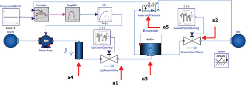
The system measures five physical quantities measured throughout a 2000-s simulation of this system, which are labeled “a1” through “a5,” shown via red arrows in Fig. 1, and are detailed in Table I.

TABLE I Description of Simulation Variables, Proprietary System

Name	Variable Description
a1 $({\mathrm{m}}^3/\mathrm{s})$	Volumetric flow through “UpstreamValve” block
a2 $({\mathrm{m}}^3/\mathrm{s})$	Volumetric flow through “DownstreamValve” block
a3 $(\mathrm{W})$	Power of flow from “Reservoir” block
a4 $(\mathrm{kg}/\mathrm{s})$	Mass flow through “pipe” block
a5 $(\mathrm{bar})$	Relative pressure in “Reservoir” block

In Table I, “a1” refers to the volumetric flow, in cubic meters per second, at the outlet of the “UpstreamValve” block wherein the opening of the valve is randomized at each time step, as determined by “UpstreamOpening.” That is, the upstream valve’s opening changes with time to allow different levels of flow at each time step; the valve may be open 90% at t = 1 s and 85% at t = 2 s. Likewise, “a2” refers to the volumetric flow through the “DownstreamValve” block, which undergoes the same unsteady operation as the upstream valve. The valves were modeled as unsteady to add large levels of process noise to the simulation. The total power, or work done per unit time, measured in, of water flowing through the reservoir is labeled as “a3.” Note that “Power of flow” is a quantity given directly from the simulation that refers to the product of the time derivative of total fluid volume, in cubic meters per second, and the system’s ambient pressure (taken as atmospheric conditions). The mass flow rate, in kg/s, through the “‘Pipe’” block is shown as “a4” in Fig. 1, which refers to the rate at which water is pumped from the source. Note that this variable will be nearly equivalent to a1 aside from a scaling factor. The relative pressure, in bars, of the water in the reservoir is shown as “a5” in Fig. 1.

Each variable, with the exception of a5, directly measures the water flow rate at various locations throughout the system. The volumetric flow rate is directly taken for a1 and a2, and a3 and a4 consider the power of flow and the mass flow rate, respectively, to differentiate the scale of each variable. For instance, a3 is measured on the order of 1e+4 W while a1 is on the order of 0.1 m³/s. While this subtle distinction bares no physical or behavioral impact on the remainder of the analyses, it is important to show that a variety of variables and values may be masked without compromising downstream utility.

The generic data, i.e., the data to be utilized in Eq. (2)(2) $y_G\left(x^{\prime },{\alpha }^{\prime }\right)\approx {\displaystyle \sum _{\mathit{i}=1}^r{\psi }_i^G\left(x^{\prime }\right)}{\varphi }_i^G\left({\alpha }^{\prime }\right)$(2) for the remainder of experimentation, are also based on a pre-rendered Open Modellica simulation seen in Fig. 2. By design, the generic data are meant to be open source, so the model is used directly, with no major changes from documentation.^[27] Once again, there are five variables taken from this system, hereinafter referred to as the generic system, that are labeled as “b1” through “b5,” shown in Fig. 2 and detailed in Table II. Briefly, the generic system comprises water that flows from an infinite sink in response to relative pressure changes throughout the system rather than via the pump. Several branching pipes are designed with different pressure drops and heated to different levels; e.g., the “pipe8” component is continuously heated from an external source.

TABLE II Description of Simulation Variables, Generic System

Name	Variable Description
b1 $({ }^{\circ }\mathrm{C})$	Fluid temperature, “pipe8” outlet
b2 $(\mathrm{kJ})$	Enthalpy flow, “pipe6” outlet
b3 $(\mathrm{N})$	Force of friction, “pipe6” outlet
b4 $(\mathrm{g}/\mathrm{c}{\mathrm{m}}^3)$	Fluid density, “pipe4” outlet
b5 $(\mathrm{bar})$	Differential pressure, “valve1”

Fig. 2. Generic System, Series of Heated Pipes. Variables, b1 through b5, labeled with Red Arrows.

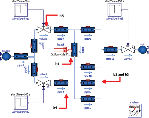
The fluid temperature at the outlet of “Pipe8” is labeled “b1” in Figure 2. The enthalpy flow, in, of liquid through “Pipe6” is shown as “b2.” Note that enthalpy flow denotes the change in total energy over time (i.e., the change in potential, kinetic, and internal energy at each successive timestep). The force of friction at the outlet of “Pipe6” is shown as “b3.” The fluid density over time at the outlet of “Pipe4” is shown as “b4,” which will change slightly over the course of the simulation due to large temperature changes. The differential pressure, in, between the inlet and outlet of “Valve1” is shown as “b5.”

The experiments in the following sections will each use the generic system exactly as described above and will each modify the proprietary system. The reader should note that these modifications, which will be detailed in the following sections, are taken only to exemplify their respective experiments and are not specifically meant to adhere to realistic principles (beyond the simulation) or a real-world system.

IV. PROMINENT ANOMALY CASE

The first experiment, which is hereinafter referred to as the Prominent Anomaly Case, considers several instances of downstream leakage, that are modeled by the openings of four independent valves, hereinafter referred to as anomalous valves, added to the proprietary system and labeled “AnomalousValve1” through “AnomalousValve4,” respectively, in Fig. 3 and highlighted in gray. Four anomalous valves are specified so that there are several independent instances of excess flow rate throughout the simulation for various durations and magnitudes.

Fig. 3. Proprietary System Modified for the Prominent Anomaly Case. Anomalous Valves Highlighted in Gray as “AnomalousValve1” through “AnomalousValve4” whose openings are determing by “AnomalousLeakage1” through “AnomalousLeakage4.”

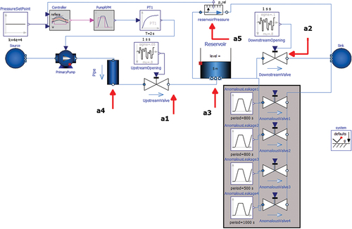
Each valve is opened at preset intervals, detailed in columns 1 through 4 in Table III. Column 1 denotes which valves are open. Column 2 denotes the maximum allowed mass flow rate through each valve. Column 3 denotes the duration of each valve opening as well as when they are opened. For example, “20 (100, 900)” denotes that “AnomalousValve1” is opened from t = 100 to 120 s and t = 900 to 920 s. Column 4 denotes the number of total instances that will occur for that valve. An “anomaly” is triggered as soon as any of these valves is opened, and behavior is considered “normal” only when they are all fully closed. A partially open anomalous valve is still counted as an anomaly for this experiment. Note that the maximum allowed flow rate through “AnomalousValve1” and “AnomalousValve2” is comparable to that of the normal upstream and downstream valves.

TABLE III Details of Pipe Leakage Anomalies, Prominent Anomaly Case

Anomaly Description	Maximum Mass Flow (kg/s)	Duration, Start Times (s)	Number of Instances
AnomValve1 is open	1000	20 (100, 900)	2
AnomValve2 is open	400	75 (1200, 1400, 1600)	3
AnomValve3 is open	1000	100 (1000)	1
AnomValve4 is open	400	200 (400)	1

This experiment considers the scenario in which anomalies are easily identifiable to act as a base case for the remainder of this paper’s experiments. The condition monitoring problem is easily performed.

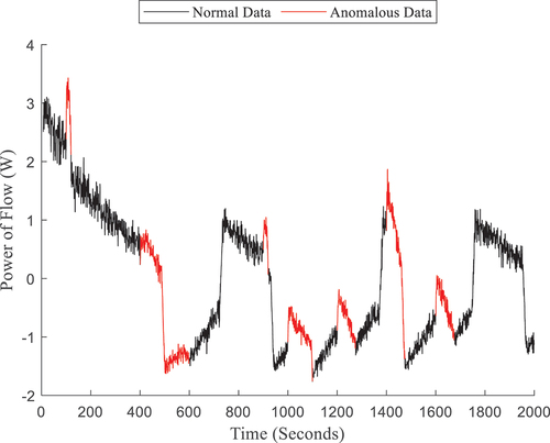
For the modified system, the power of flow from the reservoir is shown in Fig. 4 wherein the data are labeled “0” and colored black for any given time step when all anomalous valves are closed, meaning that the only flow is due to the upstream and downstream valves, i.e., normal behavior. The anomalous behavior is colored in red and labeled “1,” i.e., the times when at least one anomalous valve is open, meaning that there is an increased flow rate to the sink.

Fig. 4. Prominent Anomaly Case, Power of Flow through the Reservoir.

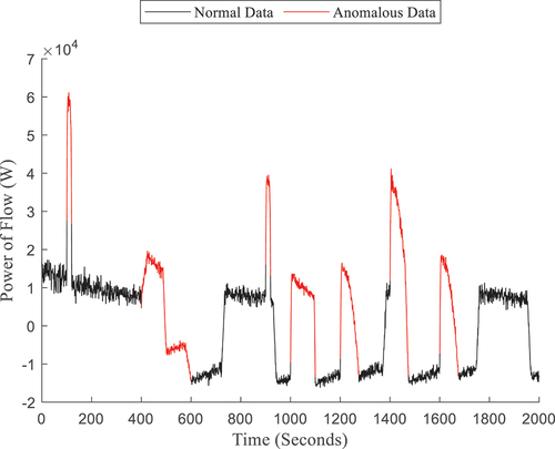
If an analyst notes that the anomalous characteristics are reflected by large increases in the flow rate, each anomalous region in Fig. 4 is clearly visible without necessitating the use of a classifier. The reader should, however, note the difference between anomalous events (colored in red) and piecewise regions that are produced by the activity of the primary pump, in response to decreasing water height. Because of the size of the anomalies in this case, anomalous leakage typically causes pump action, e.g., the anomaly from t = 400 to 600 s, but occasionally will not, e.g., t = 100 s.

Before proceeding with the experiment, it is necessary to briefly view the masked data, i.e., data produced via Eqs. (1)(1) $y_P\left(\mathit{x},\mathit{\alpha }\right)\approx \sum _{\mathit{i}=1}^r{\psi }_i^P\left(\mathit{x}\right){\varphi }_i^P\left(\mathit{\alpha }\right)$(1) , (2)(2) $y_G\left(x^{\prime },{\alpha }^{\prime }\right)\approx {\displaystyle \sum _{\mathit{i}=1}^r{\psi }_i^G\left(x^{\prime }\right)}{\varphi }_i^G\left({\alpha }^{\prime }\right)$(2) , and (3)(3) $\begin{array}{c}{y}_D\left(\mathit{x}{ }^{\mathrm{\prime }},\mathit{\alpha }\right)=\sum _{\mathit{i}=1}^r{\psi }_i^G\left(\mathit{x}{ }^{\mathrm{\prime }}\right){\varphi }_i^P\left(\mathit{\alpha }\right)\end{array}.$(3) . Recall that Eq. (1)(1) $y_P\left(\mathit{x},\mathit{\alpha }\right)\approx \sum _{\mathit{i}=1}^r{\psi }_i^P\left(\mathit{x}\right){\varphi }_i^P\left(\mathit{\alpha }\right)$(1) is based on the decomposition of the proprietary data and Eq. (2)(2) $y_G\left(x^{\prime },{\alpha }^{\prime }\right)\approx {\displaystyle \sum _{\mathit{i}=1}^r{\psi }_i^G\left(x^{\prime }\right)}{\varphi }_i^G\left({\alpha }^{\prime }\right)$(2) is, likewise, based on the generic data produced by the system in Fig. 2. A sample feature of the generic data can be seen in Fig. 5, which shows the temperature of fluid at the outlet of “pipe8.” The reader should note the different time axis of Fig. 5, which shows a 200-s simulation compared to Fig. 4, which shows a 2000-s simulation.

Fig. 5. Generic Data, Temperature of Fluid at Pipe 8.

Given the two sets of data, Eq. (3)(3) $\begin{array}{c}{y}_D\left(\mathit{x}{ }^{\mathrm{\prime }},\mathit{\alpha }\right)=\sum _{\mathit{i}=1}^r{\psi }_i^G\left(\mathit{x}{ }^{\mathrm{\prime }}\right){\varphi }_i^P\left(\mathit{\alpha }\right)\end{array}.$(3) is applied to form the masked data, shown in Fig. 6. The reader should note that the generic data are noiseless, composed of low-frequency fundamental trends, and have no class labels. As noted in Sec. II, the noise level and complexity of either dataset does not fundamentally limit DIOD, but the masked data will often reflect the noisier of the two datasets. That is, the masked data formed in this experiment should have high levels of noise, though it may be comparatively less than Fig. 4 because of the noiseless behavior of Fig. 5.

Fig. 6. Prominent Anomaly Case, Masked Power of Flow through the Reservoir.

While different in appearance, the same timesteps are labeled “0” and “1” for Figure 4 and Figure 6, meaning that the same anomalies occur, and can be seen in the masked data. Note that the masked data is, broadly speaking, similar to the original data. This is partially due to the choice of generic data in Figure 5, which was from a similar simulation without the presence of noise. However, the data’s scale, temporal behavior, and statistics are altered. For example, the y-axis for Fig. 4 is on the order of 10 kW while the y-axis of Fig. 6 is on the order of 1 W. Though anomalies occur at the same timesteps, the shape of the data spikes is also much different. A particular point of comparison for the reader may be the piecewise behavior of Figs. 4 and 6. The reader will note that Fig. 6 has a different number of piecewise regions than Fig. 4, thereby indicating different pump action to a knowledgeable adversary. For example, there are three piecewise regions in Fig. 4 from t = 400 to 500 s, t = 500 to 600 s, and t = 600 to 700 s, but in Fig. 6, there is only one piecewise transition from about t = 500 to 750 s. Furthermore, Figure 6 lacks the ‘steady’ regions of Figure 4. To a knowledgeable adversary, this would imply a physically unstable system where the direction and magnitude of flow rate are constantly changing.

While Fig. 6 shows that the temporal profile of the data changes via obfuscation, the intervariable correlations should also be shown. Figure 7 compares the value at each time step of the volumetric flow rate through the downstream valve (a2), in cubic meters per second, and the power of flow from the reservoir (a3), in watts. As previously noted, the scale of the y-axis in Figure 4 is several orders of magnitude larger than that of Figure 6, so variables must be re-scaled for convenient interpretation. Each variable is normalized via standardization to zero mean and unit variance for the ease of interpretation. The reader will note that the red and black clusters in Fig. 7 are almost completely distinct, meaning that the correlations of the data have been heavily altered. Thus, Figs. 4, 6, and 7 show that both temporal behavior and intervariable relationships are altered by the masking process so that no “hints” are given to reverse engineer the DIOD process.

Fig. 7. Prominent Anomaly Case, volumetric flow through “DownstreamValve” versus power of flow from “Reservoir.”

V. SUBTLE ANOMALY CASE

While Sec. IV experiments with large, easily classifiable anomalies, it is often the case that real process anomalies occur over a longer duration and are more difficult to identify. While several large and independent events may be trivial to identify in this system, the impact of the so-called subtle anomaly, which is physically present as minor excess valve leakage, is minimal and thus may be harder to detect over a much longer portion of the simulation. By injecting a smaller anomaly, such as very small pipe leakage, its behavior is much closer to the inherent noise of the system than a significant anomaly. As such, the condition monitoring problem is much more complex, and it is important to assess whether DIOD will still preserve the anomaly.

The second experiment, referred to hereinafter as the Subtle Anomaly Case, models a small process variation in the same experimental system as the previous section with altered parameters to suit this problem. For this experiment, the subtle anomaly is caused only by the opening of the “AnomalousValve1” component and all other anomalous valves remain closed for the entire simulation. The anomalous period is split into two cycles starting at 100 and 900 s, respectively; i.e., the anomaly occurs at t = 100 to 600 s and t = 900 to 1400 s.

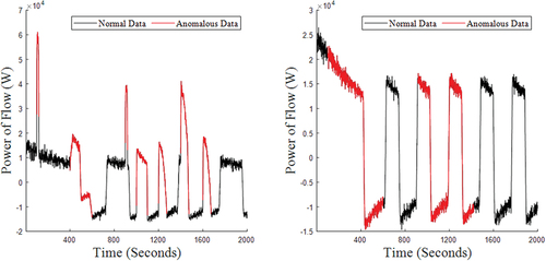
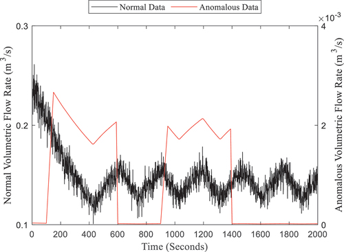
Figure 8 shows the power of flow through the central reservoir for the Prominent Anomaly Case on the left, and for the Subtle Anomaly Case on the right. Note that the left subplot of Figure 8 is a re-stated version of Figure 4 for ease of comparison. As previously noted, the Prominent Anomaly Case contains easily identifiable anomalies via large data spikes. In contrast, it is much more difficult to identify distinctly anomalous behavior from the right figure since there are no clear spikes. While the pump is turned on and off several times in each figure, which is shown via from the sharp discontinuities, it is unclear from the right figure whether any of this behavior is necessarily due to an anomaly, even when distinctly anomalous regions are highlighted in red.

Fig. 8. Comparison of power of flow through reservoir across experiments. Left, Prominent Anomaly Case (restatement of Fig. 4). Right, Subtle Anomaly Case.

To further illustrate this point for the Subtle Anomaly Case, Fig. 9 compares the volumetric flow through the downstream valve, with the power of flow from the reservoir, from the original data only where the black data points are normal behavior and red is anomalous. Similar to Fig. 8, however, it is difficult to tie the highlighted regions to anomalous behavior. To illustrate why the subtle anomaly in this experiment is so well hidden, Figure 10 compares the magnitudes of volumetric flow through the downstream valve with the flow rate through the anomalous valve, which are denoted in the left and right y-axis, respectively. The flow rate through the anomalous valve is 2-3 orders of magnitude below the flow rate through the downstream valve and the two flow rates do not appear to share any time-dependent relationship.

Fig. 9. Subtle Anomaly Case, Volumetric Flow through the Downstream Valve vs. Power of Flow through the Reservoir.

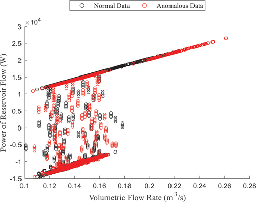
Fig. 10. Subtle Anomaly Case, Volumetric Flow through the Downstream Valve Colored in Black, Volumetric Flow through AnomValve1 Colored in Red.

VI. MULTI-REGIME ANOMALY CASE

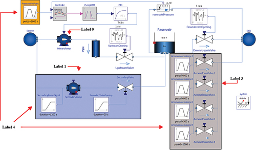
The third experiment, referred to hereinafter as the Multi-Regime Anomaly Case, further expands the previous scenarios by implementing several independent behavioral regimes for a 5000-s simulation, compared to the 2000-s simulation previously. The modified system, shown in Fig. 11, is consistent with previous experiments except for two major additions that contribute to newly formulated behavior. The first, highlighted in orange, is the inclusion of an unsteady set point for the controller action, which is labeled “PressureSetPoint.” A secondary pump, highlighted in blue, is added to act as a second regime of normal behavior during the second half of the simulation. Once again, the four anomalous valves, highlighted in gray, will still be opened at several preset times (these times differ from the Prominent Anomaly experiment).

Fig. 11. Proprietary System Modified for the Multi-Regime Anomaly Case. Controller Set Point Highlighted in Orange, Secondary Pump Highlighted in Blue, Anomalous Valves Highlighted in Gray.

While Secs. IV and V dealt with a binary label given to a classifier, i.e., “0” for normal behavior and “1” for anomalous behavior, the Multi-Regime Anomaly Case involves six independent labels in order to confirm that DIOD preserves the inferential content of several behavioral regimes. The details of each label are given in Table IV.

TABLE IV Description of Anomalous Regimes

Label	Description	Time (s)	Proportion (%)	Number of Instances
0	“PrimaryPump” operating normally, “SecondaryPump” is off, all “AnomalousValves” closed	5 to 105, 405 to 800, 1000 to 1795,	25.8	3
1	“PrimaryPump” and “SecondaryPump” operating normally, all “AnomalousValves” closed	3795 to 5000	24.1	1
2	“PrimaryPump” failure	105 to 405	6	1
3	At least one “AnomalousValve” is open	800 to 1000, 2223 to 2905, 3205 to 3795	29.5	3
4	“SecondaryPump” operating, at least one “AnomalousValve” is open, and “PrimaryPump” failure	2905 to 3205	6	1
5	Postprocess noise addition	1795 to 2223	8.6	1

Briefly, Label 0 refers to standard behavior wherein the “PrimaryPump” block is operating normally (i.e., responding to a fixed setpoint) and all “AnomalousValve” components are closed. This state is consistent with the normal behavior of previous experiments and will occur in the first 2500 s of the simulation, except when interrupted by anomalies. Label 1 refers to standard behavior during the second half, i.e., t = 2500 to 5000 s, of the simulation wherein all “AnomalousValve” blocks are closed, the controller responds to a constant signal, and both pumps are active. The newly added secondary pump, shown as the “SecondaryPump” component, does not respond to any control law but will be constantly operational after t = 2500 s. Labels 0 and 1 are different states of normal behavior for the purposes of this paper, but their differences must be respected after masking, thus necessitating individual labels. The reason for this distinction is that many realistic applications may have various states of operational behavior. While they may not necessarily constitute anomalies, different operational states must be differentiated in an inferential sense. An example of this scenario is nuclear plant operating at 80% and 90% of its rated power.

Label 2 denotes a failure in the primary pump that occurs during the first half of the simulation, i.e., interrupts Label 0, wherein the “PressureSetPoint” block that is responsible for maintaining water height in the reservoir is set to 0 bars. Because of this, the PrimaryPump shuts off and does not respond to water height when it should, otherwise, be active. Label 3 refers to several instances wherein at least one anomalous valve is open at any point in the simulation, i.e., interrupts either Label 0 or Label 1. Note that the definition of Label 3 here is equivalent to the definition of “anomalous” in Secs. IV and V.

Label 4 refers to the overlap of Labels 1, 2, and 3; i.e., the primary pump fails during the second half of the simulation when at least one anomalous valve is also open. The significance of this anomaly is that it will convey properties from each label at the same time. It is considered as a separate label to examine whether DIOD will respect compounding anomalous behavior. In theory, the behavior of Label 4 is distinct from its individual components, but it may be possible that it is misclassified as Label 2 (or split between Label 2 and Label 3). Once again, it is crucial to the theoretical evaluation of DIOD that a classifier can differentiate Label 4 from Labels 1, 2, and 3. If in the opposite case, Label 4 is identified with 100% accuracy in the original data but only 50% accuracy in the masked data, then DIOD has failed to preserve inference.

Label 5 (which is not shown in Fig. 11) refers to the addition of post-process white noise to the power of flow from the reservoir. Though not associated with any component of the simulation or physical process, this anomaly is added to the experiment to assess the impact of exogenous behavior and to assess whether it will also be conveyed during masking. Once again, this anomaly investigates an important facet of DIOD in any realistic scenario: If DIOD cannot convey the impact of noise from outside the simulation, then it has failed to preserve all inferential content.

Figure 11 shows the primary component associated with each label (apart from Label 5, which does not correspond to any component), and Table IV summarizes each label. column 1 denotes the label type, column 2 gives a brief description, column 3 denotes the active times of each label, column 4 shows the proportion of total data that occupy each label, and column 5 denotes the number of occurrences of each label. For example, row 1 describes Label 0, which occurs during the simulation at the times noted in column 3 and occupies 25.8% or (1290) seconds of the total data split into three separate occurrences. From column 4, it should be noted that Labels 0, 1, and 3 comprise most of the data while the remaining labels occupy relatively minor proportions.

VII. RANDOMIZED LABELS

The final experiments examine a scenario in which labeling information is lost. Using Fig. 11, there are two scenarios where (1) the labels from t = 1233 s to t = 2470 s are randomized and (2) all labels are randomized throughout the entire simulation. These are referred to as the “Partially Randomized Labels Case” and the “Fully Randomized Labels Case,” respectively. In either case, “randomized labels” refers to a replacement of the original labeling information with a uniformly random integer from 0-5. For instance, if t = 10 seconds originally belonged to Label 1, it is replaced with a random integer from 0-5. Note that the range t = 1233 to 2470 s is arbitrarily assigned and will corrupt the labeling information of Labels 0, 3, and 5. By randomizing the labels across some interval, the ability of a classifier in these experiments will be diminished in proportion to the number of labels that is replaced. As such, the performance of a condition monitoring algorithm is strongly weakened due to poor training. Within the randomly shuffled regions of the data, a random guess from 0–5 will give approximately 16.7% accuracy for the corrupted label.

These scenarios seek to examine whether DIOD is still usable in a case where information is incomplete or has been corrupted. It is important to confirm that, even in this case, DIOD does not arbitrarily add information. This conclusion may only be drawn if the loss in information is equivalent in the original and masked data. In other words, these experiments examine whether classification accuracy decreases by the same amount in the original and masked data in both experiments. If DIOD does not rely on a well-determined system/group of labels, it can be applied to a broader range of experimental data where there are large uncertainties and possible measurement gaps, thus further expanding applicable use cases.

VIII. EXPERIMENTAL RESULTS AND DISCUSSION

Following the discussion of each experiment in Secs. III through Sec. VII, this paper will conclude with a comprehensive evaluation and comparison of each result. The metric of comparison is classification performance, which is defined for this paper as the ability of a well-trained classifier to correctly identify the label at each time step. To test a variety of experiments, this section will consider three types of classifiers, all implemented using the MATLAB software, version 2023b: a neural-network (NN) architecture, a k-nearest neighbors (KNN) classifier, and a support vector machine (SVM).^[28–32]

Each classifier is structured to train with (to learn from) 90% of the dataset and tested on (does not learn from) 10% of the data. For this paper, ten trials are repeated for each experiment wherein a new classifier is trained using re-randomized assignments of the training and testing data for each trial. That is, for each experiment (Sec. IV through Sec. VII) and classifier combination, ten independently randomized trials are conducted using newly trained classifiers for each trial. Repeated evaluation using a fixed data pool is considered to approximate the uncertainty of the classifier’s performance in each experiment for later comparison between the original and masked data. The classifiers are evaluated by the accuracy of their labeling, i.e., the proportion, as a percentage, of labels that are correctly identified. For example, 80% accuracy shows that, across all time steps and all labels, 80% are labeled correctly and 20% are mislabeled. Since ten trials are performed, each result is displayed using the average classifier accuracy and its associated error bounds as μ±σ. In each trial, classifier performance is gauged by the accuracy of the model during training, hereinafter the training accuracy, and the accuracy of the model using the remaining 10% of data not seen by the model during training, hereinafter the testing accuracy.

The reader should also note that a consistent classifier architecture is used in each respective case so that aside from the data and labels utilized as input, nothing varies from trial to trial for the sake of consistency. Since the goal of this paper is not to optimize the classification procedure, no attempt is made to investigate deeper networks or optimize the parameters of any given classifier. Each classifier is implemented via MATLAB functions from the Classification Learning Toolbox, and brief details are given as follows.^[33]

A NN classifier uses an array of individual neurons to iteratively fit the labeled data and is capable of learning nonlinear trends. Briefly, each neuron is interconnected so that the output of a given neuron depends on every preceding neuron. For example, if the input populates five neurons, then in the next layer, each neuron’s output is decided by a weighted sum of these five inputs. As such, each neuron in the so-called hidden layer (the layers of neurons between the input and the output) is separately parameterized. For each case in this paper, the network architecture consists of a two-layer feedforward neural architecture (the layers contain 25 and 10 neurons, respectively) with rectified linear unit activation layers.

The KNN classifier defines clusters of a user-specified number of points with the lowest distance to one another that share consistent labeling information.^[30] By isolating closely related information, the model defines several independent decision boundaries, i.e., separations between different class labels, well suited to predicting unknown labels. New data are assessed in terms of their distance from each cluster’s centroid. That is, if the input data are close to a particular centroid, this maximizes the likelihood that a given point shares that cluster’s labeling information. The KNN architecture utilized for these experiments considers 10 nearest neighbors wherein pointwise distance is defined in the Euclidean sense and given a squared inverse weighting factor (meaning that neighbors far away from the centroid of a given cluster have a minimal impact).

An SVM classifier defines a decision boundary by finding the optimal linear decision boundary in a higher-dimensional space, called a hyperplane.In this case, the SVM uses a 5-dimensional plane because the data contain five features that separates the specified labeling information, thereby confidently predicting new labels. The hyperplane is defined with the objective of maximizing the distance between classes of data. The SVM architecture used in the following experiments is defined by a Gaussian kernel function, meaning that 5-dimensional hyperplanes are calculated with respect to a radial function, as opposed to a linear plane. Since SVMs are conditioned toward a binary classification, i.e., label 1 or label 0, the multi-class requirement of the experiments in Secs. VI and VII is fulfilled by assigning a binary SVM to each pair of labels (giving 15 total binary SVMs to assess the eventual six labels) and selecting the predicted label by maximizing the posterior probability, i.e., “confidence,” among possible predictions. This is done by another MATLAB function suited to the multi-class problem.^[32]

Table V is used to evaluate the first batch of results, considering the Prominent Anomaly, Subtle Anomaly, and Multi-Regime Anomaly Cases (Secs. IV, V, and VI), and gives a sequential comparison and is organized to show each classifier side by side (with accuracy measured as a percentage of correctly labeled data). For instance, the first row of results shows the classification accuracy for each trial from the Prominent Anomaly Case and is read as follows.

TABLE V Classification Accuracy of Each Experiment, Secs. IV, V, and VI

		Neural Network		k-Nearest Neighbor		Support Vector Machine
Experiment	Data	Original Data	Masked Data	Original Data	Masked Data	Original Data	Masked Data
Prominent Anomaly	Train	100 ± 0	100 ± 0	100 ± 0	100 ± 0	98.94 ± 0.05	98.98 ± 0.04
	Test	99.92 ± 0.11	99.86 ± 0.12	99.82 ± 0.13	99.82 ± 0.17	99.02 ± 0.40	98.91 ± 0.26
Subtle Anomaly	Train	95.93 ± 7.56	95.43 ± 8.29	100 ± 0	100 ± 0	63.96 ± 0.75	64.58 ± 0.56
	Test	95.39 ± 8.28	95.24 ± 8.67	98.91 ± 0.28	98.88 ± 0.39	63.47 ± 2.34	62.12 ± 1.29
Multi-Regime Anomaly	Train	99.41 ± 0.32	99.39 ± 0.32	100 ± 0	100 ± 0	94.61 ± 0.05	94.70 ± 0.06
	Test	99.31 ± 0.45	99.17 ± 0.41	99.87 ± 0.08	99.90 ± 0.07	94.46 ± 0.21	94.66 ± 0.43

For the training dataset (in the row of the “Train” cell), the first results shown are the classification accuracy of the NN, first for the training dataset of the original data and then for the training dataset of the masked data. Continuing to the right, the equivalent results are given for both the KNN and the SVM classifiers. In the next row, the same measurements are given for the testing datasets in the Prominent Anomaly Case.

According to the numerical results in Table V, every trial shows similar results when compared between the original and masked data (left-to-right). Thus, even for the noisy process-based data within this paper, various supervised classification techniques are utilized to great effect (even in the case of subtle anomalies).

Beginning with the first row, each result is consistent between the original and the masked data. That is, the mean accuracy of the original and the masked data trials appears to be mostly within the bounds of one another. For example, the testing dataset of Prominent Anomaly Case, as evaluated by the NN classifier, shows 99.92% for the original data and 99.86% for the masked data on average. Similar conclusions can be drawn from the KNN and the SVM results. Since the Prominent Anomaly Case contains easily identifiable anomalies, the near-perfect identification of anomalies should be expected, and is also shown in the masked data.

Consequently, the Subtle Anomaly Case shows a much more uncertain result in each scenario, which is to be expected due to the nature of the anomaly. Even with the increased uncertainty of classifier performance, the original and masked data still show similar mean accuracy. Furthermore, the masked data’s results also reflect the increased bounds of uncertainty across each classifier. As a particular note, there is a clear decrease in the original data’s evaluation when using the SVM, meaning that there is a large burden on the analyst to properly validate their model. While it appears that the masked data carries the proper inferential content in every scenario, note that the masked data does not change the complexity of the condition monitoring process and this validation must still be performed will not necessarily make training/optimization easier.

Finally, the Multi-Regime Case supports the above conclusions wherein the original and the masked data show similar accuracy and uncertainty in each classifier. This is a particularly meaningful result since it shows that both additive (i.e., Label 4, which was caused by the overlapping occurrence of Labels 1, 2, and 3) and exogenous white noise do not compromise DIOD’s inferential guarantees.

The remaining experiments, discussed in Sec. VII, consider randomized labels. Recall that the purpose of this scenario is to confirm that the masked data, under the assumption of corrupted information by way of incorrect labels, lose approximately the same amount of information, as the original data. This is a crucial experiment to confirm that an arbitrary addition of information is not added to the masked data, thereby confirming the consistency of either dataset. As noted previously, this case uses the data from the Multi-Regime Case, whose results are restated in the first row of Table VI (this is the same as the last row of Table V, provided for ease of interpretation). Table VI should be read the same way as Table V.

TABLE VI Classification Accuracy of Randomized Labels, Multi-Regime Case

		Neural Network		k-Nearest Neighbor		Support Vector Machine
Experiment	Data	Original Data	Masked Data	Original Data	Masked Data	Original Data	Masked Data
Multi-regime anomaly	Train	99.41 ± 0.32	99.39 ± 0.32	100 ± 0	100 ± 0	94.61 ± 0.05	94.70 ± 0.06
	Test	99.31 ± 0.45	99.17 ± 0.41	99.87 ± 0.08	99.90 ± 0.07	94.46 ± 0.21	94.66 ± 0.43
Partially randomized labels	Train	79.22 ± 0.43	79.40 ± 0.24	100 ± 0	100 ± 0	75.94 ± 0.06	75.59 ± 0.13
	Test	78.83 ± 0.92	78.74 ± 0.86	79.47 ± 0.72	79.58 ± 0.76	75.08 ± 0.62	75.37 ± 1.09
Fully randomized labels	Train	19.24 ± 0.34	19.56 ± 0.40	100 ± 0	100 ± 0	17.95 ± 0.13	18.13 ± 0.14
	Test	17.05 ± 0.68	16.76 ± 1.15	16.67 ± 1.18	16.16 ± 0.58	16.28 ± 0.51	16.53 ± 0.78

First, the accuracies of the original and the masked data are, once again, very consistent across each scenario. As noted in Table VI, the training accuracy of the KNN is nearly 100% in each case, but testing accuracy tends toward the expected lower value (and is consistent with the NN and SVM). Broadly speaking, this is a symptom of overfit which causes loss in model generalizability. However, for the purposes of this paper, the more relevant comparison is between the original and the masked data. Table VI shows that DIOD will perform as expected, even in the case of corrupted/incorrect information. As in Table V, this conclusion is supported by comparing the columns of each experiment. For example, the testing accuracy in the Partially Randomized Labels Case for a NN is about 78.83% for the original data and 78.74% for the masked data with comparable bounds of uncertainty.

IX. CONCLUSION

The increased vulnerability of high-velocity industrial data in the wake of AI/ML tools has become a growing concern across a variety of industries and end-use cases. While countless techniques can provide data protection from unknown parties at the network level, most notably encryption, only a select number of state-of-the-art methods successfully address the concern of trustworthiness. Collaboration’s typical requirement of proprietary data exchange imposes massive liabilities due to potential trustworthiness concerns, public-facing portions of the stakeholder/industry, and the additional security concerns of a third party. The previously proposed DIOD paradigm expanded upon in this paper secures the data without the limiting assertions of similar techniques.

This paper expands the capabilities of DIOD by considering high-fidelity simulation data of a simple leaking reservoir simulation from Open Modellica. The primary motivation of this paper has been to show that DIOD preserves the information associated with a variety of time-dependent anomalies. The first experiment considered prominent anomalies occurring at various intervals during which the masked data were shown not only to convey anomalous information but also to visually convey a departure from standard behavior at the same time steps. The classification accuracy, or number of anomalies successfully identified, is nearly 100% with low bounds of uncertainty for both the original and masked data. The second experiment limited analysis to a subtle anomaly that occured over a much longer duration. Once again, the mean classifier accuracy was maintained in the masked data. It should be noted that the uncertainty of each classifier’s performance in the Subtle Anomaly Case was much higher than the Prominent Anomaly Case, which was also reflected in the masked data.

In the remaining experiments, several anomalies were added to the system in the Multi-Regime Anomaly Case, where it was shown that DIOD maintains inferential properties among all labels. This observation is especially noteworthy since one of the anomalies considered the addition of white noise, thus ensuring that DIOD will also preserve the impact of exogenous behavior. The final experiments investigated two levels of data corruption, wherein the associated labels were randomized over a select portion and the entire simulation, respectively. These cases, which both maintained classifier accuracy, showed that DIOD will not artificially add or subtract information, even in several cases where observations were incomplete/incorrect. Furthermore, all five major experiments conducted in this paper were also tested (with the same associated procedures) in a KNN and SVM classifier architecture, wherein there was no major change in experimental conclusions. While the validity of various classifiers depends heavily on the data, optimization by an analyst, and use case (e.g., SVMs are well suited to the Multi-Regime Anomaly Case but not to the Subtle Anomaly Case), the masked data consistently maintained the inferential conclusions associated with the original data in each respective scenario and across each classifier.

Several intended experiments and papers will be part of future work to expand upon the use case, results, and applicability of DIOD. This paper has discussed a specific time series dataset, and further experimentation with different dynamic systems is ongoing. The authors particularly note the importance of nonlinear systems to future work. Another major study will consider the extent of DIOD’s behavioral changes to the data by assessing the impact of different (possibly randomized) generic data sets and their applicability to the masked data in terms of covertness.

Acknowledgments

Idaho National Laboratory is a multiprogram laboratory operated by Battelle Energy Alliance, LLC for the U.S. Department of Energy under contract number DE-AC07-05ID14517. This work of authorship was prepared as an account of work sponsored by an agency of the U.S. Government. Neither the U.S. Government, nor any agency thereof, nor any of their employees makes any warranty, express or implied, or assumes any legal liability or responsibility for the accuracy, completeness, or usefulness of any information, apparatus, product, or process disclosed, or represents that its use would not infringe privately owned rights. The U.S. Government retains, and the publisher, by accepting the article for publication, acknowledges that the U.S. Government retains a nonexclusive, paid-up, irrevocable, worldwide license to publish or reproduce the published form of this paper, or allow others to do so, for U.S. Government purposes. The views and opinions of authors expressed herein do not necessarily state or reflect those of the U.S. Government or any agency thereof.

Disclosure Statement

No potential conflict of interest was reported by the author(s).

Additional information

Funding

This work was supported by the Idaho National Laboratory, Department of Energy, Light Water Sustainability Program [DE-AC07-05ID14517].

Notes

¹ A.Al Rashdan and H.Abdel-Khalik, Deceptive Infusion of Data, Non-Provisional Patent, Application No. 63/227,389, September 2022.

APPENDIX

Table A.I summarizes each variable in Eqs. (1)(1) $y_P\left(\mathit{x},\mathit{\alpha }\right)\approx \sum _{\mathit{i}=1}^r{\psi }_i^P\left(\mathit{x}\right){\varphi }_i^P\left(\mathit{\alpha }\right)$(1) , (2)(2) $y_G\left(x^{\prime },{\alpha }^{\prime }\right)\approx {\displaystyle \sum _{\mathit{i}=1}^r{\psi }_i^G\left(x^{\prime }\right)}{\varphi }_i^G\left({\alpha }^{\prime }\right)$(2) , and (3)(3) $\begin{array}{c}{y}_D\left(\mathit{x}{ }^{\mathrm{\prime }},\mathit{\alpha }\right)=\sum _{\mathit{i}=1}^r{\psi }_i^G\left(\mathit{x}{ }^{\mathrm{\prime }}\right){\varphi }_i^P\left(\mathit{\alpha }\right)\end{array}.$(3) (as they are discussed in Sec. II).

TABLE A.I Description of Variables in Eqs. (1)(1) $y_P\left(\mathit{x},\mathit{\alpha }\right)\approx \sum _{\mathit{i}=1}^r{\psi }_i^P\left(\mathit{x}\right){\varphi }_i^P\left(\mathit{\alpha }\right)$(1) , (2)(2) $y_G\left(x^{\prime },{\alpha }^{\prime }\right)\approx {\displaystyle \sum _{\mathit{i}=1}^r{\psi }_i^G\left(x^{\prime }\right)}{\varphi }_i^G\left({\alpha }^{\prime }\right)$(2) , and (3)(3) $\begin{array}{c}{y}_D\left(\mathit{x}{ }^{\mathrm{\prime }},\mathit{\alpha }\right)=\sum _{\mathit{i}=1}^r{\psi }_i^G\left(\mathit{x}{ }^{\mathrm{\prime }}\right){\varphi }_i^P\left(\mathit{\alpha }\right)\end{array}.$(3)

Variable	Description
$\mathit{x}$	General form of the temporal/spatial variable within the proprietary data [e.g., at $\mathit{x}=\left(5,9\right)$ may refer to five units across a one-dimensional space and at $\mathit{t}=9$ s into a given process].
$\mathit{\alpha }$	General form of the process parameters associated with the proprietary data. Intuition is similar to the state variables of a dynamic system (i.e., underlying parameters informing the behavior of the data with respect to its typical form). Depending on the problem, $\mathit{\alpha }$ may involve physical values (e.g., temperature, pressure, etc.) or material conditions (type, enrichment, etc.).
$x^{\prime }$	General form of the temporal/spatial dependence of the generic data.
${\alpha }^{\prime }$	General form of the process parameters associated with the generic data.
$y_P\left(\mathit{x},\mathit{\alpha }\right)$	The observed value of the proprietary data at some $\mathit{x}$ and $\mathit{\alpha }.$
$y_G\left(\mathit{x}{ }^{\mathrm{\prime }},\mathit{\alpha }{ }^{\mathrm{\prime }}\right)$	The observed value of the generic data at some $x^{\prime }$ and ${\alpha }^{\prime }.$
$y_D\left(\mathit{x}{ }^{\mathrm{\prime }},\mathit{\alpha }\right)$	The observed value of the masked data at some $x^{\prime }$ and $\mathit{\alpha }.$ Note the masked data do not reflect a real system and carry the same inference as $y_P$ associated with $\mathit{\alpha }$ but do not give any information about $\mathit{x}$ or $y_P\left(\mathit{x},\mathit{\alpha }\right).$
${\varphi }^P\left(\mathit{\alpha }\right)$	Proprietary inferential metadata; a subset of the data in response to some $\mathit{\alpha }$ that is relevant to inferential problems (e.g., regression, condition monitoring, etc.).
${\psi }^P\left(\mathit{x}\right)$	Proprietary fundamental metadata; a subset of the dataset in response to a temporal/spatial value of $\mathit{x}$. While this gives some description of the data’s shape and behavior (i.e., periodic, parabola, etc.), it is not referring to an individual variable or snippet of the data.
${\varphi }^G\left(\mathit{\alpha }{ }^{\mathrm{\prime }}\right)$	Generic inferential metadata; a subset of the generic dataset in response to some parameter ${\alpha }^{\prime }$ relevant to inferential content. This subset is discarded within DIOD.
${\psi }^G\left(\mathit{x}{ }^{\mathrm{\prime }}\right)$	Generic fundamental metadata; a subset of the generic dataset in response to temporal/spatial value of $\mathit{x}{ }^{\mathrm{\prime }}$. This informs the overall behavior of the generic data but is NOT an individual variable or section of the data. This will inform the shape/behavior of the masked data after using Eqs. (1)(1) $y_P\left(\mathit{x},\mathit{\alpha }\right)\approx \sum _{\mathit{i}=1}^r{\psi }_i^P\left(\mathit{x}\right){\varphi }_i^P\left(\mathit{\alpha }\right)$(1) , (2)(2) $y_G\left(x^{\prime },{\alpha }^{\prime }\right)\approx {\displaystyle \sum _{\mathit{i}=1}^r{\psi }_i^G\left(x^{\prime }\right)}{\varphi }_i^G\left({\alpha }^{\prime }\right)$(2) , and (3)(3) $\begin{array}{c}{y}_D\left(\mathit{x}{ }^{\mathrm{\prime }},\mathit{\alpha }\right)=\sum _{\mathit{i}=1}^r{\psi }_i^G\left(\mathit{x}{ }^{\mathrm{\prime }}\right){\varphi }_i^P\left(\mathit{\alpha }\right)\end{array}.$(3) .

References

- A. M. ELTAMALY et al., “IoT-Based Hybrid Renewable Energy System for Smart Campus,” Sustainability, 13, 15, 8555 (2021); https://doi.org/10.3390/su13158555.
- M. RÄMÄ, M. LEURENT, and J. D. DE LAVERGNE, “Flexible Nuclear Co-Generation Plant Combined with District Heating and a Large-Scale Heat Storage,” Energy, 193, 116728 (2020); https://doi.org/10.1016/j.energy.2019.116728.
- J. MA et al., “Research on Data Leakage Prevention Technology in Power Industry,” Proc. 6th Int. Conf. Smart Grid and Smart Cities (ICSGSC), Chengdu, China, 2022, p. 43 (2022); https://doi.org/10.1109/ICSGSC56353.2022.9963127.
- K. S. SON, J. G. SONG, and J. W. LEE, “Development of the Framework for Quantitative Cyber Risk Assessment in Nuclear Facilities,” Nucl. Eng. Technol., 55, 6, 2034 (2023); https://doi.org/10.1016/j.net.2023.03.023.
- A. ELAKRAT and J. C. JUNG, “Development of Field Programmable Gate Array–Based Encryption Module to Mitigate Man-in-the-Middle Attack for Nuclear Power Plant Data Communication Network,” Nucl. Eng. Technol., 50, 5, 780 (2018); https://doi.org/10.1016/j.net.2018.01.018.
- B. PENG et al., “A Mixed Intelligent Condition Monitoring Method for Nuclear Power Plant,” Ann. Nucl. Energy, 140, 107307 (2020); https://doi.org/10.1016/j.anucene.2020.107307.
- M. N. ALENEZI, H. ALABDULRAZZAQ, and N. Q. MOHAMMAD, “Symmetric Encryption Algorithms: Review and Evaluation Study,” Int. J. Commun. Netw. Inf. Secur., 12, 2, 256 (2020); https://doi.org/10.17762/ijcnis.v12i2.4698.
- E. SHMUELI et al., “Database Encryption: An Overview of Contemporary Challenges and Design Considerations,” SIGMOD Rec., 38, 3, 29 (2010); https://doi.org/10.1145/1815933.1815940.
- L. ZHOU et al., “Security Analysis and New Models on the Intelligent Symmetric Key Encryption,” Comput. Secur., 80, 14 (2019); https://doi.org/10.1016/j.cose.2018.07.018.
- X. YI, R. PAULET, and E. BERTINO, “Homomorphic Encryption,” Homomorphic Encryption and Applications, pp. 27–46, Springer, Cham (2014); https://doi.org/10.1007/978-3-319-12229-8_2.
- C. DWORK, “Differential Privacy: A Survey of Results,” Proc. 5th Int. Conf. Theory and Applications of Models of Computation (TAMC 2008), Xi’an, China, April 25–29, 2008, p. 1, Springer (2008); Lecture Notes in Computer Science, Vol. 4978, p. 1, Springer, Berlin, Heidelberg (2008); https://doi.org/10.1007/978-3-540-79228-4_1.
- J. HSU et al. “Differential Privacy: An Economic Method for Choosing Epsilon,” Proc. 27th Computer Security Foundations Symp., Vienna, Austria, July 19–22, 2014, p. 398, IEEE (2014); https://doi.org/10.1109/CSF.2014.35.
- D. BOGDANOV, R. TALVISTE, and J. WILLEMSON, “Deploying Secure Multi-Party Computation for Financial Data Analysis,” Financial Cryptography and Data Security, pp. 57–64, Springer, Berlin, Heidelberg (2012); https://doi.org/10.1007/978-3-642-32946-3_5.
- W. ZHANG and X. LI, “Data Privacy Preserving Federated Transfer Learning in Machinery Fault Diagnostics Using Prior Distributions,” Struct. Health Monit., 21, 4, 1329 (2022); https://doi.org/10.1177/14759217211029201.
- A. DING, G. MIAO, and S. S. WU, “On the Privacy and Utility Properties of Triple Matrix-Masking,” J. Priv. Confidentiality, 10, 2 (2021); https://doi.org/10.29012/jpc.674.
- P. S. PISA, M. ABDALLA, and O. C. M. B. DUARTE, “Somewhat Homomorphic Encryption Scheme for Arithmetic Operations on Large Integers.” Proc. Global Information Infrastructure and Networking Symp. (GIIS), Choroni, Venezuela, December 17–19, 2012, p. 1, IEEE (2012); https://doi.org/10.1109/GIIS.2012.6466769.
- K. R. SAJAY, S. S. BABU, and Y. VIJAYALAKSHMI, “Enhancing the Security of Cloud Data Using Hybrid Encryption Algorithm,” J. Ambient Intell. Humaniz. Comput. (2019); https://doi.org/10.1007/s12652-019-01403-1.
- M. YANG et al., “Local Differential Privacy and Its Applications: A Comprehensive Survey,” (2020); https://doi.org/10.48550/arXiv.2008.03686.
- P. C. M. ARACHCHIGE et al., “Local Differential Privacy for Deep Learning,” IEEE Internet Things J., 7, 7, 5827 (2020); https://doi.org/10.1109/JIOT.2019.2952146.
- A. SUNDARAM, H. ABDEL-KHALIK, and A. AL RASHDAN, “Deceptive Infusion of Data: A Novel Data Masking Paradigm for High-Valued Systems,” Nucl. Sci. Eng., 196, 8, 911 (2022); https://doi.org/10.1080/00295639.2022.2043542.
- A. AL RASHDAN et al. “A Novel Data Obfuscation Method to Share Nuclear Data for Machine Learning Application,” Light Water Reactor Sustainability Program, INL/RPT-22-69871, Idaho National Laboratory (2022); https://lwrs.inl.gov/Advanced%20IIC%20System%20Technologies/NovelDataObfuscationMethodShareNuclearData.pdf.
- M. GARRIDO, K. K. PARHI, and J. GRAJAL, “A Pipelined FFT Architecture for Real-Valued Signals,” IEEE Trans. Circuits Syst. I, 56, 12, 2634 (2009); https://doi.org/10.1109/TCSI.2009.2017125.
- Y. LANG et al., “Reduced Order Model Based on Principal Component Analysis for Process Simulation and Optimization,” Energy Fuels, 23, 3, 1695 (2009); https://doi.org/10.1021/ef800984v.
- W. ZHANG and M. WEI, “Model Order Reduction Using DMD Modes and Adjoint DMD Modes,” Proc. 8th AIAA Theoretical Fluid Mechanics Conf., Denver, Colorado, June 5–9, 2017, American Institute of Aeronautics and Astronautics (2017); https://doi.org/10.2514/6.2017-3482.
- P. FRITZSON et al., “The OpenModelica Integrated Environment for Modeling, Simulation, and Model-Based Development,” MIC J., 41, 4, 241 (2020); https://doi.org/10.4173/mic.2020.4.1.
- “Pumping System,” Modelica Association (2020); https://github.com/modelica/ModelicaStandardLibrary/blob/master/Modelica/Fluid/Examples/PumpingSystem.mo.
- “Incompressible Fluid Network,” Modelica Association (2020); https://github.com/modelica/ModelicaStandardLibrary/blob/master/Modelica/Fluid/Examples/IncompressibleFluidNetwork.mo.
- The MathWorks, Inc. (2023); MATLAB version: 23.2.0 (R2023b). Available: https://www.mathworks.com
- “Fitcnet, Train Neural Network Classification Model,” MathWorks; https://www.mathworks.com/help/stats/fitcnet.html ( current as of Nov. 11, 2023).
- “Fitcknn, Fit k-Nearest Neighbor Classifier,” MathWorks; https://www.mathworks.com/help/stats/fitcknn.html ( current as of Nov. 11, 2023).
- “Fitcsvm, Train Support Vector Machine Classifier for One-Class and Binary Classification,” MathWorks; https://www.mathworks.com/help/stats/fitcsvm.html ( current as of Nov. 11, 2023).
- “Fitcecoc, Fit Multi-Class Models for Support Vector Machines or Other Classifiers,” MathWorks; https://www.mathworks.com/help/stats/fitcecoc.html ( current as of Nov. 11, 2023).
- “Classification Learner, Train Models to Classify Data Using Supervised Machine Learning,” Statistics and Machine Learning Toolbox, MathWorks; https://www.mathworks.com/help/stats/classificationlearner-app.html ( current as of Feb. 27, 2024).
APPENDIX
summarizes each variable in EquationEqs. (1)(1)
(1) , Equation(2)
(2)
(2) , and Equation(3)
(3)
(3) (as they are discussed in Sec. II).
TABLE A.I Description of Variables in EquationEqs. (1)(1)