Estimating men’s fertility from vital registration data with missing values

Abstract

Comparative perspectives on men’s fertility are still rare, in part because vital registration data are often missing paternal age information for a substantial number of births. We compare two imputation approaches that attempt to estimate men’s age-specific fertility rates and related measures for data in which paternal age information is missing for a non-negligible number of cases. Taking births with paternal age information as a reference, the first approach uses the unconditional paternal age distribution, while the second approach considers the paternal age distribution conditional on the maternal age. To assess the performance of these two methods, we conduct simulations that mimic vital registration data for Sweden, the United States, Spain, and Estonia. In these simulations, we vary the overall proportion and the age selectivity of missing values. We find that the conditional approach outperforms the unconditional approach in the majority of simulations and therefore should be generally preferred.

Keywords:

• men’s fertility
• birth register data
• imputation methods
• Sweden
• United States
• Spain
• Estonia

Introduction

Much of the fertility literature has focused on women’s reproduction, while research on men’s reproduction has remained rare (Coleman 2000; Poston et al. 2006). However, interest in men’s fertility has been growing due to an increasing involvement of men in fertility decision-making and parenting (Lappegård et al. 2011), and in response to concerns that have been raised about possible links between paternal age and the health outcomes of children (Paavilainen et al. 2016; Khandwala et al. 2017). The number of studies that analyse men’s fertility has therefore been growing in recent years (e.g., Lappegård et al. 2011; Carmichael 2013; Nisén et al. 2014; Nordfalk et al. 2015; Dudel and Klüsener 2016; Schoumaker 2017).

One important reason for comparative perspectives on men’s fertility being rare is that in vital registration data paternal age information is often missing for a substantial proportion of births, which makes it difficult to estimate age-specific fertility rates (ASFRs) and summary measures such as the total fertility rate (TFR) for men. According to the United Nations Department of Economic and Social Affairs (UN DESA 2014), the proportions of missing values for paternal age in the birth registers of European countries in recent years have ranged from lows of around 1–2 per cent in countries such as Slovenia and Sweden, to a value of nearly 30 per cent in Lithuania. In Latin America, even higher values for missing paternal age have been recorded: for example, 35 per cent of births in Uruguay and 71 per cent in Ecuador.

When estimating men’s fertility for countries where paternal age information is lacking for a substantial number of births, it is very common to impute the missing ages based on the paternal age distribution among births for which this information is available. This approach is used by the UN DESA (2014), among others. For example, if 8 per cent of births with paternal age information have a father aged 30, then it is assumed that this pattern also applies to births with missing paternal age data. This approach ignores the likely possibility that paternal age information is not ‘missing completely at random’ (Heitjan and Basu 1996). There is strong evidence for this, which relies on a variable that is virtually always available for registered births: the age of the mother. In many data sets, maternal age at birth is highly correlated with both the probability of a missing value and the age of the father. More specifically, the paternal age is less likely to be recorded if the birth is to a young mother, while for most cases of a birth to a young mother for which paternal age information is available, the father is also relatively young (see ‘The conditional approach’ subsection later). It can therefore be assumed that fathers whose ages are not recorded are likely to be younger than fathers whose ages are known.

In this paper, we compare two non-parametric imputation approaches that are used to deal with missing paternal age data: the frequently applied ‘unconditional’ approach, described in the previous paragraph, and the ‘conditional’ approach. The conditional imputation approach replaces the unconditional paternal age distribution with the paternal age distribution conditional on maternal age (Carmichael 2013; Dudel and Klüsener 2016). It thus makes use of more information than the first approach and explicitly assumes that maternal and paternal ages at birth are highly correlated. If, for example, we consider births to mothers aged 30 with missing paternal age information, we can impute ages for these births by taking the observed distribution of paternal ages for mothers aged 30 into account. If 6 per cent of all births with known paternal age to mothers aged 30 are to fathers aged 30, then 6 per cent of the births with unknown paternal age to mothers aged 30 are assigned the paternal age 30.

To compare the performance of the unconditional and conditional imputation approaches, we conduct simulations that allow us to assess the bias in fertility estimates due to the proportion and age selectivity of missing values. These simulations mimic empirical birth register data for Sweden (1968–2014), the United States (US) (1969–2015), Spain (1975–2014), and Estonia (1989–2013), and thus represent realistic settings. The countries and years cover very different demographic conditions, ranging from relatively early and high fertility to late and lowest-low fertility. These variations in conditions allow us to explore the strengths and weaknesses of both approaches. The TFR for women in Sweden over the last few decades has been compared to a rollercoaster, with a succession of increases and decreases (Hoem and Hoem 1996; Andersson and Kolk 2016). In the US, the TFR was around two for most of our observation period, after an initial decline. The Spanish TFR plummeted from a rather high value in the late 1970s to a level of lowest-low fertility (Kohler et al. 2002), and has been consistently below 1.5 since the 1990s. Estonia’s TFR dropped quickly after the collapse of the Soviet Union, in part due to the postponement of births to older ages. All the countries in our study have seen marked increases in the mean age at childbirth for women, albeit from rather different baseline levels and with varying intensities. For overviews of women’s fertility trends in the countries studied, see the supplementary material (section 2).

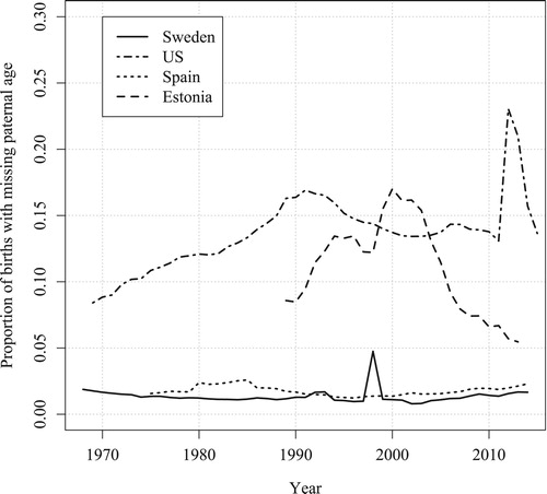
The proportion of births with missing paternal age fluctuates considerably in the countries and years we study (Figure 1). For instance, the proportion is about 1–2 per cent in Sweden for most years, but as high as 17 per cent for the US in the early 1990s. More generally, for the US and Estonia, the proportion of missing values is above 10 per cent in most years, while it is always below 5 per cent for Sweden and Spain. Differences between countries and years can be driven by many factors. These include cross-national variation in regulations as to whether mothers are obliged to provide information on the father (this often varies for marital and non-marital births; see, e.g., Dudel and Klüsener 2016 for Germany) and the degree of willingness of mothers to give information on the father if they are not required to. Sometimes, changes in the timelines of administrative processes to obtain the annual statistics can also cause variation in the share of missing values. For instance, in Sweden in 1998 the proportion of missing values was considerably higher compared with the preceding and following years. The reason for this is that the statistics for 1998 were derived from the birth register very early in 1999 due to procedural changes. At that time, paternal ages were still missing for a considerable share of non-marital births, as mothers are given a fixed period after the initial registration in which they can add any missing information on the father (Statistics Sweden, personal correspondence, 16 February 2018).

Figure 1 Trends in the proportion of births with unknown paternal age, Sweden (1968–2014), US (1969–2015), Spain (1975–2014), and Estonia (1989–2013)

Source: Statistics Sweden, National Bureau of Economic Research, Spanish Statistical Office, Statistics Estonia, Human Mortality Database; own calculations.

The remainder of this paper is structured as follows. In the ‘Imputation methods’ section, we explain the unconditional and conditional approaches. In the ‘Simulation study set-up’ section, we describe the data we use and how the simulation is set up. Next, we present the ‘Results’, followed by a ‘Summary and conclusion’.

Imputation methods: Formal definitions

Notation

We are interested in calculating ASFRs for a given country and year, $t$. The count of births to men aged $x$ is denoted by $B(x,t)$—that is, births in the age interval $[x,x+1)$, during the time interval $[t,t+1)$—while $N(x,t)$ refers to the population exposure of men aged $x$. ASFRs are calculated as $f(x,t)=B(x,t)/N(x,t)$. To simplify the notation, we drop $t$ and write, for example, $f\left(x\right)$.

To avoid any issues with the denominator of fertility rates, we assume that $N\left(x\right)$ is always known. The number of births with missing paternal age is denoted by $B{(}^{\ast })$. Since paternal age is unknown for some births, it may be assumed that the data on age-specific birth counts, $B\left(x\right)$, are not complete. Instead, only $B^O\left(x\right)$ is observed; this captures the births for which paternal age is known to be $x$. If there are missing values, $B^O\left(x\right)$ will be lower than $B\left(x\right)$.

The unconditional approach

The unconditional approach is based on the assumption that paternal age at birth is ‘missing completely at random’, which means that the probability of a missing value does not depend on the age of the father or on other variables in the birth register. Births with missing values for paternal age, $B{(}^{\ast })$, are then distributed according to the observed paternal age distribution (see, e.g., UN DESA 2014). Written formally, let $P^O\left(x\right)$ denote the proportion of births to fathers aged $x$, calculated by ignoring missing values; that is, $P^O\left(x\right)=B^O\left(x\right)/{\sum }_{i=\alpha }^{\text{β}}{B}^O\left(i\right)$, where $\alpha$ and $\text{β}$ are the youngest and oldest ages, respectively, of the reproductive phase for men. The unconditional approach then calculates ASFRs as:$f\left(x\right)=\frac{B^O\left(x\right)+B{(}^{\ast }\left)P^O\right(x)}{N\left(x\right)}.$

The conditional approach

The conditional approach assumes that in many cases, paternal age information is not ‘missing completely at random’. For instance, for Sweden from 1968 to 2014, the Spearman’s rank correlation between the proportion of missing values and the age of the mother is −0.4. Similar negative correlations can also be obtained for the other three countries. As we stated earlier, the conditional approach exploits the correlation between maternal age at birth and both paternal age at birth and the probability of a missing value. It does so by using the paternal age distribution conditional on the age of the mother (Carmichael 2013; Dudel and Klüsener 2016). This is based on the assumption that the age of the father is ‘missing at random’ conditional on the age of the mother (as opposed to ‘missing completely at random’). More formally, let $B^O(x,y)$ denote the number of births to fathers aged $x$ and mothers aged $y$. We assume that maternal age is virtually always available, which, based on the data documentation of the Human Fertility Database (2018), seems to be quite a realistic assumption. $P^O\left(x\right|y)$ is the observed paternal age distribution conditional on maternal age, calculated as $B^O(x,y)/{\sum }_{i=\alpha }^{\text{β}}{B}^O(i,y)$, and $B{(}^{\ast },y)$ represents the number of births with known maternal age (that equals $y$), but unknown paternal age. ASFRs are then calculated as:$f\left(x\right)=\frac{B^O\left(x\right)+{\sum }_{j=\gamma }^{\delta }B{(}^{\ast },j\left)P^O\right(x\left|j\right)}{N\left(x\right)}$where $\gamma$ and $\delta$ denote the youngest and oldest childbearing ages for women.

Simulation study set-up

Data

To achieve realistic results, our simulation study emulates real data based on empirical birth counts, age distributions, and population exposures. To derive the birth counts and age distributions of mothers and fathers, we use birth register data from Sweden (1968–2014; supplied by Statistics Sweden), the US (1969–2015; available through the National Bureau of Economic Research), Spain (1975–2014; provided by the Spanish Statistical Office), and Estonia (1989–2013; supplied by Statistics Estonia). For the US, the data for some years are based on 50 per cent random samples from the birth registers of individual US states. For these years, we use weights to estimate the number of births by maternal and paternal ages. The population exposures for all the countries are taken from the Human Mortality Database (2018).

Simulation set-up

To assess the relative performance of each method, we simulate data that mimic important characteristics of the actual birth register data. These characteristics include observed paternal age at birth distributions conditional on maternal age at birth in each country and year. The simulation set-up is briefly presented here, while further details and discussions are provided in the Appendix. In our simulated data sets, we know the paternal ages for all births, but assume that they are unobserved for some births. We consider a wide variety of simulations in which we change two parameters: (1) the overall proportion of missing values; and (2) a parameter that alters the paternal age distribution for those births with missing paternal age. This second parameter, called ‘age shift’, explores how the performance of our methods changes if the unobserved paternal age distribution of births with missing values differs from the observed distribution. For instance, if the age shift parameter equals −1 year, this means that the average paternal age for births with missing values is one year lower than for births with known paternal age (see the Appendix for a discussion of alternative strategies). If this age shift parameter is different from zero, then the missing values are not ‘missing at random’, which implies that the assumptions of both the unconditional and conditional approaches are violated.

We refer to data for a specific country–year combination as a simulation setting, of which we have 159 in total. For each simulation setting, we apply 450 different combinations of simulation parameters, resulting in a total of 71,550 simulations. For the proportion of missing values, we use values of 1–50 per cent with 1 per cent increments; while for the age shift, we consider values from −4 years to +4 years with one-year increments. Age shift values below −2 and above +2 can be considered rather extreme (see the Appendix for a discussion).

For each of our 71,550 simulations, we simulate two data sets: one representing the ‘observed’ data with missing values and the other representing the ‘true’ underlying data without missing information. These two data sets are identical except for one aspect: some births for which paternal age is known in the ‘true’ data have missing values in the ‘observed’ data. To generate the data sets, we start with all births for a given country and year, and then distribute them on a preliminary basis according to $P^O\left(x\right|y)$, that is, the paternal age distribution conditional on maternal age. The latter has been calculated for the same country and year based on the empirical births for which the paternal age is known. Then we make use of the first parameter, the proportion of missing values, to set the age of the father to ‘missing’ for some births. This share ‘missing’ varies by the age of the mother, for which we again mimic characteristics in the specific country–year simulation setting. For births for which the age of the father is ‘observed’, we keep the empirical age distribution $P^O\left(x\right|y)$. The resulting data set consists of the ‘observed’ simulation data. To introduce age selectivity among the births with ‘unobserved’ paternal age, we shift the originally simulated paternal age for each of these births according to the age shift parameter. The combined ‘observed’ and (shifted) ‘unobserved’ parts of the data then become the ‘true’ data set that we can use as a benchmark to measure the performance of the two imputation approaches.

To assess the bias of each imputation method, we calculate the men’s total fertility rate (MTFR) and the paternal mean age at childbirth (PMAC), both based on the ‘true’ data, as well as the MTFR and PMAC based on the ‘observed’ data where missing paternal ages have been imputed with one of the two approaches. We then calculate the absolute bias of both imputation approaches for the MTFR and the PMAC as $|\text{MTF}{\text{R}}_{\mathrm{t}\mathrm{r}\mathrm{u}\mathrm{e}}-\text{MTF}{\text{R}}_{\mathrm{o}\mathrm{b}\mathrm{s}\mathrm{e}\mathrm{r}\mathrm{v}\mathrm{e}\mathrm{d}}|$ and $|\text{PMA}{\text{C}}_{\mathrm{t}\mathrm{r}\mathrm{u}\mathrm{e}}-\text{PMA}{\text{C}}_{\mathrm{o}\mathrm{b}\mathrm{s}\mathrm{e}\mathrm{r}\mathrm{v}\mathrm{e}\mathrm{d}}|$, respectively. Bias in the MTFR captures whether the level of fertility is estimated correctly, while bias in the PMAC allows us to assess whether the timing of fertility is estimated correctly.

Results

Illustrative example: Sweden 2014

We use the simulation results based on the recent Swedish data for 2014 as an illustrative example that allows us to explain how the simulations and imputation approaches work. In other years and countries, both higher and lower values of bias can be found (see the next subsection and the supplementary material (section 1)).

The simulation results for Sweden in 2014 are shown in Figures 2–5. Figure 2 displays the absolute bias of the MTFR estimate derived using the unconditional imputation approach, and the extent to which it depends on both the proportion of missing values and the selectivity of missing values (age shift). Figure 3 shows the same information for the conditional imputation approach. Absolute bias never exceeds 0.012 on the MTFR scale; that is, the difference between the ‘true’ MTFR and the MTFR based on imputation is never higher than 0.012 points for either approach and is thus small. If the proportion of missing values is below 10 per cent, bias is negligible for both approaches, irrespective of the age shift. In the case of the unconditional method, the results are biased to some extent above this threshold, even if there is no selectivity at all among the missing values.

Figure 2 Absolute bias of the men’s total fertility rate (MTFR) in MTFR points, based on the unconditional approach to estimating paternal age, by age shift and proportion missing; simulations for Sweden, 2014

Source: Own calculations.

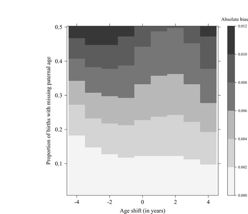
Figure 3 Absolute bias of the men’s total fertility rate (MTFR) in MTFR points, based on the conditional approach to estimating paternal age, by age shift and proportion missing; simulations for Sweden, 2014

Source: Own calculations.

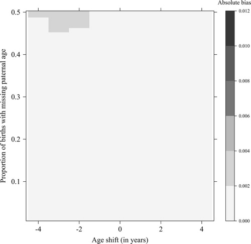
In contrast, the conditional approach performs considerably better and the degree of bias is minimal in this simulation setting, even with high age shift values. This is because the conditional approach correctly accounts for the higher probability that missing values will occur among younger mothers, who have younger partners on average. If the fathers are a few years older or younger than is estimated by the conditional approach—as indicated by the age shift parameter—these discrepancies usually have little effect on the degree of bias in the MTFR estimate. This is because the MTFR is sensitive to inaccuracies in the paternal age imputation only if successive cohorts vary substantially in size, which is rarely the case. The overall performance of the conditional approach is considerably better than that of the unconditional approach, as in 97 per cent of our simulations based on Swedish data for 2014, the former approach is less biased than the latter.

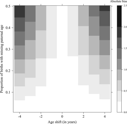
Figures 4 and 5 show the absolute bias for the estimates of the PMAC. For this measure, in contrast to the MTFR, paternal age information is the key determinant of the calculations. The overall pattern is quite different from the pattern found for the MTFR, as the conditional approach outperforms the unconditional approach in this simulation setting in only 56 per cent of the simulations. The level of bias in the PMAC can be considerable for both methods, amounting to a maximum difference of 2.2 years between the ‘observed’ and ‘true’ values for the unconditional approach, and to a maximum difference of 1.9 years for the conditional approach. For the conditional approach, the level of bias seems to be more balanced around an age shift of zero and is high only for more extreme values of the age shift parameter. Meanwhile, for the unconditional approach the bias can be more than one year for an age shift of +2.

Figure 4 Absolute bias of the paternal mean age at childbirth (PMAC), based on the unconditional approach to estimating paternal age, by age shift and proportion missing; simulations for Sweden, 2014

Source: Own calculations.

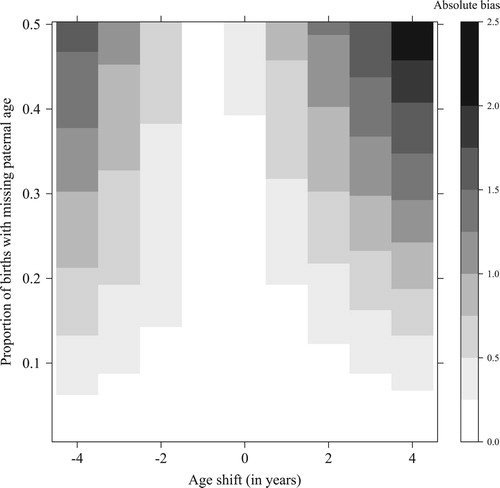
Figure 5 Absolute bias of the paternal mean age at childbirth (PMAC), based on the conditional approach to estimating paternal age, by age shift and proportion missing; simulations for Sweden, 2014

Source: Own calculations.

Simulation results for Sweden, the US, Spain, and Estonia

For each of our 159 country–year combinations, we generated results like those presented in Figures 2–5. A more detailed breakdown of these results is available in the supplementary material (sections 1 and 3), while Table 1 gives an overview. For each country, the proportion of simulations in which the conditional approach outperforms the unconditional approach is shown for both the MTFR and the PMAC. In columns 1 and 4 we provide the outcomes for all the parameter combinations considered. In addition, we present the results for more limited parameter spaces, in which we exclude extreme cases of age selectivity of missing values and focus only on the simulations for which the proportion of missing values is non-negligible so that the choice of approach is more relevant. Based on the detailed outcomes presented in the supplementary material (section 1), we choose here to focus on the simulations for which paternal age information is simulated to be missing for at least 10 per cent of the births. For these restricted summaries, we consider age shift parameters between −2 and +2 (columns 2 and 5), and between −1 and +1 (columns 3 and 6). The last row of Table 1 provides the average results for all the 159 country–year simulation settings considered.

Table 1 Proportion of simulations in which the conditional approach for estimating paternal age at childbirth outperforms the unconditional approach; by country and total (percentages)

	Men’s total fertility rate (MTFR)			Paternal mean age at childbirth (PMAC)
Column number	1	2	3	4	5	6
Criteria for inclusion
Age shift	−4 to +4	−2 to +2	−1 to +1	−4 to +4	−2 to +2	−1 to +1
Proportion missing	Any	>10 per cent	>10 per cent	Any	>10 per cent	>10 per cent
Percentage of simulations in which conditional approach outperforms unconditional approach
Sweden (1968–2014)	76	83	91	56	62	69
US (1969–2015)	75	92	97	73	94	100
Spain (1975–2014)	72	83	95	66	78	97
Estonia (1989–2013)	55	66	78	59	67	78
Average	71	83	92	64	76	86

Notes: Columns 1 and 4 take age shift values between −4 and +4 into account. Columns 2 and 5 are restricted to simulations with age shift values between −2 and +2, and also consider only simulations in which paternal age is missing for more than 10 per cent of births. Columns 3 and 6 cover age shift values between −1 and +1, and a proportion of missing values of at least 10 per cent.

Source: Own calculations.

While the results differ somewhat by country, the conditional approach outperforms the unconditional approach in roughly two out of three cases if all our parameter combinations are considered (columns 1 and 4). The outperformance of the conditional approach becomes even more pronounced if we consider only simulations in which at least 10 per cent of the values are missing and restrict the age shift to between −2 and +2 years (columns 2 and 5), and then to between −1 and +1 year (columns 3 and 6). Especially in the latter case, the conditional approach is highly dominant.

Summary and conclusion

We conducted simulations to compare two non-parametric imputation approaches that can be used to calculate age-specific fertility rates for men if paternal age information is missing for some births: the unconditional approach and the conditional approach. The conditional approach imputes the missing paternal age conditional on the maternal age, while the unconditional approach ignores this information. The unconditional approach, which is often adopted in the literature, can perform poorly if the proportion of missing values is non-negligible; it can be biased even if there is no selectivity of missing values. The conditional approach, on the other hand, performs better in the majority of simulations. Both approaches work well if the proportion of missing values is small. Generally, the conditional approach should be preferred, and we encourage data suppliers either to apply the conditional approach directly, or to make raw data broken down by both maternal and paternal age available, which would allow use of the conditional approach.

While our study covered several different countries and periods, one limitation is that we only mimicked data from high- and middle-income countries. It is thus unclear whether our findings are transferable to low-income countries, and especially to low-income countries where very different patterns of men’s fertility have been reported (e.g., polygamy). In addition, reliable register data are often unavailable in these countries and data quality can be low. Schoumaker (2017) has discussed how men’s fertility can be estimated in such settings.

This paper focused only on maternal and paternal ages at birth, but additional attributes could be included in both the unconditional and conditional approaches. For instance, if the legal marital status of the mother were available for every birth and had been shown to be related to the probability that the paternal age is missing, the data could be split into marital and non-marital births, and the imputation could proceed separately for each part. In such a case, however, the additional covariates would have to cover virtually all births, with no or only a few missing values. In addition, the imputation approaches presented could also be used to impute other missing information on the father (such as education or other socio-economic status attributes), provided this information is available for most of the mothers.

ORCID

Christian Dudel http://orcid.org/0000-0002-2985-6684

Sebastian Klüsener http://orcid.org/0000-0003-0436-3565

Notes

1 Please direct all correspondence to Christian Dudel, Max Planck Institute for Demographic Research, Konrad-Zuse-Str. 1, 18057 Rostock, Germany; or by E-mail: [email protected]

2 We thank Pavel Grigoriev, Kryštof Zeman, two anonymous reviewers, members of the Population Studies editorial board, conference participants in Turku (Nordic Demographic Symposium), and conference participants in Cape Town (International Population Conference) for very helpful suggestions and comments on earlier versions of the manuscript. We also thank Sigrid Gellers-Barkmann and Karolin Kubisch for data support, and Miriam Hils for language editing.

Appendix: Implementation of the simulations

For each country and year, two parameters are used to alter our simulated birth register data: the proportion of missing values for paternal age and the degree to which the age distribution of the simulated ‘unobserved’ paternal age distribution differs from the paternal age distribution among the ‘observed’ cases. These two parameters can be applied once a basic data set has been created. As we stated in the main text, we are simulating basic data sets by taking all births for a given country and year, and distributing them on a preliminary basis according to $P^O\left(x\right|y)$, that is, the paternal age distribution conditional on the maternal age distribution. The latter has been calculated for the same country and year based on the empirical births for which the paternal age is known.

The first parameter (proportion missing paternal age) is then applied by scaling the conditional proportion of missing values by the age of the mother up or down; for births with known paternal age, $P^O\left(y\right|x)$ is used. This procedure creates the simulated ‘observed’ data set with missing values. In Figure A1, the pattern found in the empirical data for Sweden in 2014 is shown as a solid line, which mostly sits at around 1–2 per cent. The dashed and dotted lines correspond to simulated overall proportions of missing values of 10 and 20 per cent. Generally, a desired proportion of missing values, $P_{\mathrm{d}\mathrm{e}\mathrm{s}}{(}^{\ast })$, is achieved by iterative upscaling: if the proportion of missing values for a country–year setting is $P_{\mathrm{o}\mathrm{b}\mathrm{s}}{(}^{\ast })$, then a scaling factor $\lambda =P_{\mathrm{d}\mathrm{e}\mathrm{s}}{(}^{\ast }\left)/P_{\mathrm{o}\mathrm{b}\mathrm{s}}{(}^{\ast }\right)$ is calculated and applied to the observed conditional proportion of missing values, resulting in a new set of adjusted values $P_{\mathrm{a}\mathrm{d}\mathrm{j}}{(}^{\ast }\left|y\right)=P_{\mathrm{o}\mathrm{b}\mathrm{s}}{(}^{\ast }\left|y\right)\lambda$.

One challenge we face is that in cases with no observed paternal ages at birth, neither the conditional nor the unconditional approach can be applied. For the conditional approach this is true even if for one or more maternal ages no births with paternal age information are available. We thus implement a ceiling so that if we derive values of $P_{\mathrm{a}\mathrm{d}\mathrm{j}}(\ast |y)$ larger than 90 per cent, the corresponding proportions are set to 90 per cent. In order to still reach the desired share of births with missing paternal age information, we use an iterative procedure in which we start anew by calculating and applying $\lambda$, potentially setting some values to 90 per cent, and again starting anew until $P_{\mathrm{d}\mathrm{e}\mathrm{s}}{(}^{\ast })\approx {(}^{\ast })$. This procedure guarantees, first, that no conditional proportion of missing values exceeds 90 per cent if the proportion is not already in the data. Moreover, in most cases, the upscaling procedure leaves the ratios of missing values unchanged; that is, $P_{\mathrm{a}\mathrm{d}\mathrm{j}}{(}^{\ast }\left|y\right)/P_{\mathrm{a}\mathrm{d}\mathrm{j}}{(}^{\ast }\left|y^{\mathrm{\prime }}\right)=P_{\mathrm{o}\mathrm{b}\mathrm{s}}{(}^{\ast }\left|y\right)/P_{\mathrm{o}\mathrm{b}\mathrm{s}}{(}^{\ast }\left|y^{\mathrm{\prime }}\right)$. For instance, if the proportion of missing values for 20-year-old women is twice as high as it is for 30-year-old women, the ratios will not be changed (except in certain cases because of the 90 per cent rule just described).

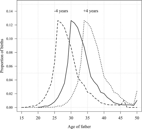
An example of the effect of the second parameter (age shift) can be seen in Figure A2; the ‘true’ data set is created using this simulation parameter. The solid line shows the distribution of paternal age conditional on the mother being aged 30 for the empirical data in 2014; that is, $P^O\left(x\right|y=30)$. As noted earlier, this is also the age distribution found in the simulated ‘observed’ data, irrespective of the overall proportion missing. The dashed line is derived by shifting the distribution of births for which we set the paternal age to missing four years to the left. This makes the fathers of births with ‘unobserved’ paternal age information younger; that is, by applying an ‘age shift’ of −4 years. The dotted line shows another scenario in which the fathers for whom paternal age is unknown are made older by shifting the distribution +4 years to the right. Formally, this shifting process can be described as follows: given an age shift of $\varphi$, the distribution of the paternal ages of births for which this information is assumed to be unobserved, $P_{\mathrm{u}\mathrm{n}}\left(x\right)$, is defined as $P_{\mathrm{u}\mathrm{n}}(x+\varphi |y)=P_{\mathrm{o}\mathrm{b}\mathrm{s}}(x\left|y\right)$. If this shift by $\varphi$ years leads to ages above $\text{β}$ (the highest age), the ages are set to $\text{β}$ and summed up; that is, $\text{β}$ functions as a ceiling. A similar procedure is applied with the bottom age, $\alpha$. This shifting approach is applied to all conditional age distributions for the age shift values from −4 to +4 in one-year increments. A value of zero implies that missing values are ‘missing at random’, while higher or lower values indicate different degrees of age-selective missingness. An age shift of −4 or +4 can be seen as rather extreme (also see Dudel and Klüsener 2016); the three distributions shown in Figure A2, for instance, imply average ages at childbirth for fathers where the mother is aged 30 of roughly 33.1 years (original data), 29.1 years (age shift of −4), and 37.1 years (age shift of +4). To put these results in perspective, it should be noted that the difference between the observed mean age and the ages implied by the shifted distributions is slightly larger than the empirical change in the mean age at childbirth for women in Sweden from 1968 to 2014.

The age shift parameter could also be implemented with distributions of different shapes from the one observed. For instance, it would be possible to combine the two shifted distributions in Figure A2 (both the dashed and dotted lines) into a bimodal mixture distribution and to use it as $P_{\mathrm{u}\mathrm{n}}\left(x\right)$, or a more skewed distribution could be chosen. However, experimenting with the shape of the distributions showed that the main driver of bias is how large the age shift is; that is, the average age and the extent to which it differs from the observed distribution. We therefore proceeded in the implementation of the age shift as described in this Appendix.

Figure A1 Proportion of missing values for age of father conditional on age of mother, Sweden 2014

Notes: Empirical data (solid line) and upscaled distributions (dotted and dashed lines). For some of the youngest and oldest ages, the 90 per cent threshold was reached and the proportion of missing values was not further increased. Source: Statistics Sweden; own calculations.

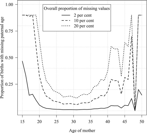
Figure A2 Distribution of age of father conditional on mother being aged 30, Sweden 2014

Notes: Original distribution (solid line) and age-shifted distributions (dotted and dashed lines). Source: Statistics Sweden; own calculations.

References

- Andersson, Gunnar and Martin Kolk. 2016. Trends in childbearing, marriage and divorce in Sweden: An update with data up to 2012, Finnish Yearbook of Population Research 50: 21–30.
- Carmichael, Gordon A. 2013. Estimating paternity in Australia, 1976–2010, Fathering: A Journal of Theory, Research, and Practice About Men as Fathers 11(3): 256–279. doi: 10.3149/fth.1103.256
- Coleman, David A. 2000. Male fertility trends in industrial countries: theories in search of some evidence, in Caroline Bledsoe, Susana Lerner, and Jane I. Guyer (eds), Fertility and the Male Life-Cycle in the Era of Fertility Decline. Oxford: Oxford University Press, pp. 29–60.
- Dudel, Christian and Sebastian Klüsener. 2016. Estimating male fertility in eastern and western Germany since 1991: A new lowest low? Demographic Research 35(Art. 53): 1549–1560. doi: 10.4054/DemRes.2016.35.53
- Heitjan, Daniel F. and Srabashi Basu. 1996. Distinguishing ‘missing at random’ and ‘missing completely at random’, The American Statistician 50(3): 207–213.
- Hoem, Britta and Jan M. Hoem. 1996. Sweden’s family policies and roller-coaster fertility, Journal of Population Problems 52(3/4): 1–22.
- Human Fertility Database. 2018. Max Planck Institute for Demographic Research (Germany) and Vienna Institute of Demography (Austria). Available: www.humanfertility.org
- Human Mortality Database. 2018. University of California, Berkeley (USA), and Max Planck Institute for Demographic Research (Germany). Available: www.mortality.org or www.humanmortality.de
- Khandwala, Yash S., Chiyuan A. Zhang, Ying Lu, and Michael L. Eisenberg. 2017. The age of fathers in the USA is rising: An analysis of 168 867 480 births from 1972 to 2015, Human Reproduction 32(10): 2110–2116. doi: 10.1093/humrep/dex267
- Kohler, Hans-Peter, Francesco C. Billari, and José Antonio Ortega. 2002. The emergence of lowest-low fertility in Europe during the 1990s, Population and Development Review 28(4): 641–680. doi: 10.1111/j.1728-4457.2002.00641.x
- Lappegård, Trude, Marit Rønsen, and Kari Skrede. 2011. Fatherhood and fertility, Fathering: A Journal of Theory, Research, and Practice About Men as Fathers 9(1): 103–120. doi: 10.3149/fth.0901.103
- Nisén, Jessica, Pekka Martikainen, Karri Silventoinen, and Mikko Myrskylä. 2014. Age-specific fertility by educational level in the Finnish male cohort born 1940–1950, Demographic Research 31(Art. 5): 119–136. doi: 10.4054/DemRes.2014.31.5
- Nordfalk, Francisca, Ulla A. Hvidtfeldt, and Niels Keiding. 2015. TFR for males in Denmark: Calculation and tempo correction, Demographic Research 32(Art. 52): 1421–1434. doi: 10.4054/DemRes.2015.32.52
- Paavilainen, Miia, Aini Bloigu, Elina Hemminki, Mika Gissler, and Reija Klemetti. 2016. Aging fatherhood in Finland—first-time fathers in Finland from 1987 to 2009, Scandinavian Journal of Public Health 44(4): 423–430. doi: 10.1177/1403494815620958
- Poston Jr., Dudley L., Amanda K. Baumle, and Michael Micklin. 2006. Epilogue: needed research in demography, in D. L. Poston and M. Micklin (eds), Handbook of Population. New York: Springer, pp. 853–881.
- Schoumaker, Bruno. 2017. Measuring male fertility rates in developing countries with Demographic and Health Surveys: An assessment of three methods, Demographic Research 36(Art. 28): 803–850. doi: 10.4054/DemRes.2017.36.28
- UN Department of Economic and Social Affairs (DESA). 2014. Demographic Yearbook 2014. New York: United Nations.