Adapting the Own Children Method to allow comparison of fertility between populations with different marriage regimes

Abstract

The Own Children Method (OCM) is an indirect procedure for deriving age-specific fertility rates and total fertility from children living with their mothers at a census or survey. The method was designed primarily for the calculation of overall fertility, although there are variants that allow the calculation of marital fertility. In this paper we argue that the standard variants for calculating marital fertility can produce misleading results and require strong assumptions, particularly when applied to social or spatial subgroups. We present two new variants of the method for calculating marital fertility: the first of these allows for the presence of non-marital fertility and the second also permits the more robust calculation of rates for social subgroups of the population. We illustrate and test these using full-count census data for England and Wales in 1911.

Keywords:

• fertility
• Own Children Method
• marital fertility
• total fertility
• age-specific fertility rate
• estimation
• historical demography
• England and Wales
• census

Introduction

In the absence of the recording of a mother’s age at the birth of her child, it is very difficult to generate age-specific fertility rates (ASFRs). The Own Children Method (OCM) for fertility estimation was first developed in the 1960s as a way of deriving estimates of age-specific and total fertility from cross-sectional census data (Grabill and Cho 1965). The OCM exploits the facts that censuses and surveys record the age of each family member, and that young children are usually recorded in the same households as their mothers. This enables the age of mothers at the births of their children to be inferred and age-specific child–woman ratios to be calculated. The method transforms these into ASFRs, using adjustments for child mortality, adult mortality among females, and children living away from their parents.

Over the last 40 years, the OCM has been frequently applied to historical census data. Full birth histories (FBHs) seldom exist for historical populations of women and it is impractical to create equivalent data through record linkage, so the OCM is frequently the most fruitful method for generating age-specific and total fertility for the past. The widening availability of big data in historical demography, with the increased digitization and harmonization of full-count census data (such as the Integrated Census Microdata (I-CeM), the Integrated Public Use Microdata Series (IPUMS), and the North Atlantic Population Project (NAPP)), has opened up more avenues for the OCM to be used on large-scale populations (Ruggles 2014).

The first demographic transition was primarily a change from fertility control by marriage to fertility control within marriage, and historical demographers are therefore particularly interested in separating out the contribution of changes in marital fertility during the fertility transition (Hinde 2003, p. 219). Although the OCM was designed to calculate overall (marital plus non-marital) fertility, it has frequently been used to calculate marital fertility, using a variety of assumptions or additional data to adjust for the role of marriage in exposing women to the risk of conception. However, these variants of the basic OCM have rarely been compared or tested for sensitivity to ways of calculating exposure. In this paper we argue that there are two main disadvantages to the commonly used variants: first, they require the strong assumption—known to be untrue in historical Europe—that all births occur within marriage (Laslett and Oosterveen 1973; Adair 1996; Muir 2018). Second, ways of calculating exposure to marriage are likely to produce distorted estimates when applied to social groups (Cho et al. 1986, pp. 30–2). This paper offers two new ways of calculating marital fertility that overcome these issues. It illustrates and tests them using big data from the 1911 Census of England and Wales, the first British census to include questions on marital duration, therefore allowing several different ways of calculating marital fertility to be compared and evaluated.

Background

The OCM was pioneered by demographers at the East–West Center for demographic research in Hawaii. It was first set out clearly in the 1960s (Grabill and Cho 1965) and subsequently refined and tested by a series of applications to different censuses and surveys, and by comparisons with other methods (Cho 1974; Rindfuss 1976, 1977; Retherford and Cho 1978, 1984; Retherford et al. 1980; Goldstein and Goldstein 1981; Retherford and Mirza 1982). The East–West Center (1992) produced a computer programme (EASWESPOP) and accompanying documentation to aid analysis, although the method is not difficult to implement. Early applications calculated fertility rates for the mid-twentieth-century United States (US), and in the 1960s and 1970s it was also widely applied to Asian countries, such as Malaysia and South Korea (Grabill and Cho 1965; Cho 1968, 1974; Rindfuss 1976, 1977). During the 1980s and 1990s, the FBHs collected by surveys such as the World Fertility Survey (WFS) and Demographic and Health Surveys (DHS) became the main source of fertility information. Comparisons between fertility estimated using WFS FBHs and the OCM from accompanying household surveys showed that the OCM produced comparable estimates, although age reporting was often better in FBHs (Retherford and Alam 1985). Some use of the OCM continued, however, with the focus moving towards the calculation of fertility differences between migrant groups in wealthy countries (Abbasi-Shavazi 1997; Dubuc 2009; Coleman and Dubuc 2010; Krapf and Kreyenfeld 2015). The method received further validation with a thorough assessment of its performance when compared with DHS data, which concluded that the OCM is generally at least as accurate as FBHs, for survey data in any case, and that selection effects can distort fertility from FBHs (Avery et al. 2013). In his more general assessment of the reliability of reverse survival methods, Spoorenberg (2014) also tested some of the more important assumptions of the OCM against a simulated population. Most recently the method has been innovatively used to produce estimates of men’s fertility (Schoumaker 2017).

Since the 1970s, the OCM has been used by historical demographers who have, of course, not benefited from the development of comparable sample surveys, and who study populations where vital registration had not yet been established or did not request information on age of mother at birth of child. For example, although vital registration was operational in England and Wales from 1837, age of mother was not recorded on birth certificates until 1938 (Higgs 2004, p. 210). Some historical applications have used the EASWESPOP program, some have used the APPLAUSI program written by historical demographers (see collection of papers in Breschi, Kurosu et al. 2003), and others have performed the calculations themselves. The method has been applied to small area census populations in the US (Hareven and Vinovskis 1975; Haines 1978, 1979), England and Wales (Woods and Smith 1983; Garrett et al. 2001; Boot 2017), and Germany (Gruber and Scholz 2016). It has also been applied to US census samples (Tolnay 1981; Tolnay et al. 1982; Tolnay and Guest 1984) and to full-count historical censuses for the US and Sweden (Hacker 2003; Scalone and Dribe 2012). Further historical studies have applied the OCM to tax registers from Tibet (Childs 2004) and fifteenth-century Florence (Breschi and Serio 2003), and to Japanese population registers (Kurosu 2003).

As with contemporary data, many historical applications have compared fertility between subgroups of the population, for example by ethnic group, migrant status, socio-economic status, and urban/rural location. There have also been a number of studies that use unadjusted numbers of young children living with their mothers in multivariate, and sometimes multilevel, models of the determinants of fertility (Haines 1978; Scalone and Dribe 2012; Dribe and Scalone 2014; Hacker 2016; Klüsener et al. 2016; Dribe et al. 2017).

There are few corroboratory data sets for historical populations against which to test the results obtained via the OCM, but nineteenth-century Swedish vital registration evidently asked questions about mother’s age, and Scalone and Dribe (2017) found that national level OCM estimates were very similar to age-specific rates calculated from vital registration data. Haines (1989) compared OCM fertility estimates to those calculated using the two-census parity increment method and found the OCM to be more robust and accurate than reported parity, particularly for older women. Breschi et al. (2003) and Oris (2003) compared fertility calculated using the OCM with that from birth histories generated from population registers (for Venice and Belgium, respectively). Both found that a failure to use the correct mortality schedule for different social or migrant groups could lead to overestimation of fertility in some groups and underestimation in others. The United Nations (UN) indirect estimation manual urges caution in interpreting OCM results for subpopulations that are not closed to migration, and the Belgian study demonstrated the compositional changes that can be produced by migration and highlighted the problems associated with population movement between areas with different mortality rates (UN 1983, p. 183; Oris 2003).

Despite these investigations, there has been little critical engagement with the way that the OCM calculates, and may distort, marital fertility. In this paper we discuss these potential issues and present new variants of the OCM for calculating marital fertility. The next section briefly describes the basic OCM for estimating overall (rather than just marital) fertility, noting the assumptions and adjustments that are commonly made. This is followed by a section detailing data we use in this paper. Then comes a section in which we use the OCM to calculate overall fertility for England and Wales (1836–1911) and review the assumptions made when using the method. Finally, we present and compare a number of different variants of the OCM for estimating marital fertility, including our two new variants.

The OCM for overall fertility: Assumptions and adjustments

In its classic form the OCM relies on matching children aged 0–14 in a census or survey with their mother in the same household. Matched children and mothers are then cross-tabulated by single years of age, and both children and mothers reverse-survived to yield annual births to woman by single years of age at birth of child. The numbers of women of each age in the population are also reverse-survived, and used as population denominators to calculate ASFRs for the 15 years leading up to the census or survey. These can be combined into five-year age groups for added robustness. Early applications of the method were performed on censuses that had a pre-coded variable specifying the number of children under age five; therefore, it was not possible to calculate annual rates, and the precise ages of women at the birth of their children could not be ascertained by back-projection (Grabill and Cho 1965). Instead, the Sprague osculatory interpolation was used to redistribute births to the correct age of mother. This procedure was also followed in some historical demography applications where small numbers of women may have made working with single-year rates more problematic (Haines 1978, 1979; Woods and Smith 1983; Hinde and Woods 1984; Garrett et al. 2001).

ASFRs and total fertility rates (TFRs) can be produced easily for subgroups, allowing comparison of fertility levels and trends over time between sections of the population for which age-specific fertility might not otherwise be easily obtained. These steps by themselves would produce accurate ASFRs and TFRs under the following assumptions:

1. There is no mortality in the population;

2. Enumeration is complete;

3. The ages of women and children are correctly reported;

4. All children under 15 live in the same household as their mother, and mother–child links have been correctly identified;

5. Children are matched to their biological mothers; and

6. Group characteristics are constant.

The extent to which violation of any of these assumptions produces bias in the estimates depends on the time and place being studied, but it is common to make adjustments to the numbers of children used in the cross-tabulations in order to: (a) take account of mortality in the years leading up to the census (inflating numbers of both women and children); (b) redistribute the children for whom a mother has not been identified; and (c) allow for the possible under-enumeration of very young children. Such adjustments of course carry their own assumptions but, having made the adjustments, we can rework assumptions 1 and 4 to make these more realistic:

• 1.1. The age distribution of the mothers of children who died is the same as the age distribution of the mothers of children who survived;

• 1.2. Women who died had similar fertility to the rest of the population; and

• 4.1. The age distribution of the mothers of very young children not recorded with their mother at census is the same as that of mothers who are recorded with their very young children.

These assumptions and adjustments will be briefly discussed as we illustrate the method with data for nineteenth- and early-twentieth-century England and Wales, as described in the next section. In particular we will discuss age misstatement and under-enumeration (assumptions 2 and 3), migration (assumption 6), mortality (assumptions 1.1 and 1.2), and ‘non-own’ children (assumptions 4.1 and 5).

Data

This research used the individual-level census returns for England and Wales for the decennial Censuses from 1851 to 1911 (excluding 1871), published and enhanced by the I-CeM project (see Appendix for further detail on I-CeM). These amount to 17.5 million individual records for 1851 and over 36 million in 1911. Numbers of children and women used for the fertility calculations are therefore extremely robust and not, at the national level, subject to small number fluctuations, even for single-year age groups. For the calculation of overall fertility from 1836 to 1911 we used all available censuses, but for the exposition of our new variants we concentrated on the 1911 Census, which, as it asked currently married women a question on the duration of that marriage, allows a more extensive comparison of different variants of the OCM for calculating marital fertility. For these comparisons we used a substantial subset of the 1911 data, consisting of those women with a plausible reported marital duration and age, and whose husband was co-resident with them on Census night. Married women with their husband present were excluded from the 1911 sample if their age or marital duration was missing, or if their age at marriage—calculated as age at Census minus marital duration—was implausible. The 1911 Census included questions on the numbers of children ever born (the number of live children ever born, the number still alive on Census night, and the number who had died), and women with inconsistent answers to these questions were also excluded. Of 6,662,862 women in the I-CeM data for 1911 who were reported to be aged 15–64 and married, 3.7 per cent were excluded due to implausible answers, either to the marital duration or one or more of the fertility questions. The majority of these instances are likely to be due to data transcription errors, which will be unbiased. A further 14.8 per cent of the women were excluded from calculations of marital fertility (variants B, C, D, and E) because they could not be linked to a husband in the same household. These women (discussed in more detail later) tended to have fewer co-resident children than women with husbands present in the household, so their omission results in slightly higher fertility estimates than if all women reported to be married are included. However, excluding these women enabled us to make comparisons between different variants of the method using exactly the same sample. The final sample used for comparative analysis of marital fertility amounts to 5,425,682 women.

For national mortality data we used single-year life tables downloaded from the Human Mortality Database (see Appendix for further detail). Subnational mortality estimates for infant mortality and early child mortality (age 1–4) were based on published mortality statistics from the Quarterly and Decennial Reports of the Registrar General (Jaadla and Reid 2017).

While many of the results we present are for England and Wales as a whole, we also calculated subnational estimates based on Registration Sub-Districts (RSDs), of which there were around 2,000 in each census year. We have classified RSDs into eight types of place, defined by their occupational structure and population density, each with a distinctive demographic regime (see Reid et al. (2018) under ‘type of place’ for more details of how these types of place were defined). In this paper we concentrate on three key types of place—professional, mining, and textile—which exhibit very different marriage patterns, as illustrated in Figure 1. Each panel in Figure 1 shows the percentage of women at each age who were married, with husband present in the same household on Census night 1911, for a specific type of place, as well as showing the percentages for England and Wales overall (E&W) for comparison. In England and Wales as a whole, and generally in the types of place not otherwise singled out in Figure 1, women married earlier than men but over a more extended range of ages, thus the slope of the ‘E&W women’ line in each panel is not as steep in its rapidly increasing phase (up until about age 30) as the line for ‘E&W men’. More striking, however, is the fact that in the population as a whole a greater proportion of women than of men remained unmarried towards the higher end of the fertile age range. The maximum proportion of women ‘married with spouse present’ occurs at around age 40, lower than the maximum for men, which occurs at ages in the mid-40s. The downturn in the proportions married at older ages predominantly reflects bereavement, which was more common among women than men due to higher mortality among men (women being usually younger than their husbands) and lower rates of remarriage after widowhood for women.

Figure 1 Percentages of men and women at each age who were married, with spouse present in the same household: three different types of place and England and Wales, 1911

Source: Authors’ calculations based on 1911 Census data from I-CeM (see Appendix for more detail on sources).

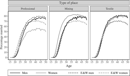
The different panels of Figure 1 show that this pattern differed between professional, mining, and textile areas in 1911. In mining places women married particularly young and were more likely to be reported as married at any age than men, an area characteristic mainly due to significant in-migration of young single men and out-migration of single women. These migration patterns are visible in the unusually high sex ratio among adults aged 20–49 in mining areas, shown in Table 1 alongside other selected demographic characteristics for England and Wales and the three types of place in 1911. High adult sex ratios are usually attributable to an imbalance of job opportunities for men and women. Professional areas, in contrast, attracted young women, who migrated in to work as domestic servants. These servants swelled the ranks of unmarried women, leading to extremely low sex ratios, low proportions of women married, and high estimates of age at marriage. Textile areas also provided plentiful work opportunities for women, but by 1911 these were mainly taken up by locals, so the proportions married were little distorted by in-migration. These different patterns of marriage are likely to have led to differing amounts of exposure to marriage among married women of the same age. For example, a married woman of age 25 in a mining area was likely to have been already married for substantially longer than a married woman of the same age in a professional area. However, if migration had a life cycle element, that is, single women migrated in to professional areas to work but left to marry and live elsewhere, it is possible that married women in professional areas actually got married at an earlier age than implied by the proportions married. It is a well-known issue that cross-sectional measures based on a synthetic cohort—such as the singulate mean age at marriage (SMAM)—can be significantly distorted by migration, especially at subnational levels (Schürer 1989). This paper considers the effect of these issues on exposure to marriage in the context of the OCM.

Table 1 Selected demographic characteristics of the population of England and Wales, and three selected types of place, 1911

	England and Wales	Type of place
		Professional	Mining	Textile
Sex ratio (20–49 years)	0.92	0.69	1.15	0.86
Population density^1	0.97	1.24	1.43	3.58
IMR^2	117.23	87.07	126.54	122.07
SMAM^3 women	26.23	28.49	24.20	26.72
SMAM^3 men	27.58	28.49	26.87	27.05
Population	36,070,492	3,222,409	3,597,665	3,270,122

¹Population density is the number of people per acre.

²IMR is the infant mortality rate: infant deaths per 1,000 births in the five years leading up to the 1911 Census (April 1906–March 1911).

³SMAM is the singulate mean age at marriage, calculated in the standard way from proportions married in the census.

Source: Authors’ calculations based on 1911 Census data from I-CeM and mortality data from the Human Mortality Database and the Quarterly Reports of the Registrar General of England and Wales (see Appendix for more detail on sources).

Using the OCM to calculate overall fertility in England and Wales

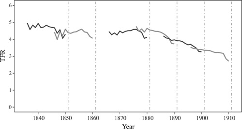
We used the individual-level data from the Censuses of 1851–1911 to derive the annual TFR series for England and Wales, 1836–1911, shown in Figure 2. Because the 1871 Census is not available there is a gap between 1861 and 1866. These estimates were calculated using the data for all women aged 15–64, together with those for children aged 0–14 years. We adjusted the figures for ‘non-own’ (unmatched) children by multiplying the number of children in each age-of-child and age-of-mother combination by the reciprocal of the proportion of children of that age who were matched to mothers. We also inflated numbers of both children and women to account for mortality. These single-year TFRs allow greater elucidation of the method and an assessment of some of the OCM assumptions laid out below.

Figure 2 Total fertility rates (TFRs) calculated using the OCM: England and Wales, 1836–1911

Notes: Vertical lines indicate the years of the six censuses used to calculate fertility. The lines showing TFRs calculated for the 15 years before each census are shown in different shades to make it easier to distinguish them from each other. The 1871 Census data are not available.

Source: Authors’ calculations based on Census data from I-CeM and mortality data from the Human Mortality Database (see Appendix for more detail on sources).

Age misstatement and under-enumeration (assumptions 2 and 3)

Each segment of line in Figure 2 is derived from a different census. The rightmost end of each segment is contributed by children aged zero (born during the year before the census), and each previous annual point is produced by children a year older, up to age 14. Ideally, we would see a smooth line with exactly overlapping segments. Jagged fluctuations usually indicate age heaping or age misstatement among children, and a lack of overlap can indicate differential under-enumeration by age and census year or faulty estimates of mortality. Figure 2 shows that the figures derived from adjacent censuses correspond relatively well. There is evidence of age heaping among older children in the earlier censuses, but this was eliminated by the end of the nineteenth century. However, the overlap between segments in Figure 2 is not perfect: in general, older children from one census indicate higher fertility than that indicated by the youngest children in the next census. There appears to have been a strong deficit of zero- and one-year-olds and a bulge of two- and three-year-olds. To some extent this can be explained by the tendency of parents to report children as the next age up (i.e., to report an eleven-month-old as a one-year-old), but it is also possible that some infants were omitted from the census forms.

We tested for age misstatement by smoothing the age distributions and found this made only a very small difference to the TFR. The possible under-enumeration of zero-year-olds, a common issue with censuses, is a potentially larger problem (Myers 1993). We tested for this using Lee and Lam’s age adjustment factors, obtaining revised estimates slightly higher than the raw ones, by 0.1–0.3 children. Lee and Lam (1983) argued that their adjustment factors for children aged 0–4 seemed implausible, and the extent of underestimation was therefore unclear. As we do not consider that the age distributions of the very young would be reliable enough to produce specific adjustment factors when working with small subgroups of the population, and because these would be further complicated by differences in migration, we decided not to adjust for possible under-enumeration. A uniform adjustment throughout would be of little benefit when comparing different groups. More detail on these tests is given in Section 1 of the supplementary material.

Migration (assumption 6)

Another potential issue for the accuracy of OCM fertility rates is the migration of young people—this is not a major issue with national data, but is potentially a problem with place-specific calculations. Such calculations (not shown here) have demonstrated that young people started to leave home for employment as servants from the age of ten or even earlier (see Schürer et al. 2018). This life cycle movement among young people results in underestimation of fertility 10–14 years before the census in agricultural districts, and overestimation in professional areas where servant-keeping was common.

In view of these considerations, most of our analyses only use children aged 0–4, who were less likely to be found living apart from their parents, and provide estimates of fertility for the five years immediately preceding each census combined. While this avoids the problem of migration of older children, we need to be aware that the under-enumeration of infants weighs more heavily when analysis is restricted to younger children.

Mortality (assumptions 1.1 and 1.2)

Various authors have assessed the impact of using inappropriate mortality levels and trends on overall and subgroup fertility. There is a general consensus that at a national level the failure to account for mortality leads to underestimates of fertility, but that mis-specification of mortality levels makes little difference and trends over time are relatively little affected (Rindfuss 1976; Retherford and Cho 1978; Retherford and Alam 1985; Cho et al. 1986; De Santis 2003; Spoorenberg 2014). However, an inability to properly account for differences in mortality among subgroups can lead to mis-specification of differences in fertility between groups (Rindfuss 1976; Retherford et al. 1980; Goldstein and Goldstein 1981; Young 1992; Oris 2003), although some have argued that this may not confound fertility differences if groups with high mortality also exhibit high fertility (Scalone and Dribe 2012; Dribe and Scalone 2014).

Section 2 of the supplementary material explains how we examined the effects of possible mis-specification of mortality, both for the overall population and for subgroups. In summary, this showed that if no mortality adjustment were made then estimates of overall fertility were 10–23 per cent too low, with the larger underestimations for earlier census years when child mortality had not yet started to fall. Similarly, underestimation was larger in settings where mortality was higher, such as mining and textile areas. Our analyses demonstrated that a 10 per cent overestimation in early age mortality resulted in fertility 5–6 per cent too high, and a 10 per cent underestimation in mortality resulted in fertility which was 6–8 per cent too low. Because the differences in mortality between our geographic areas were considerably greater than 10 per cent, and because high mortality was not always correlated with high fertility (e.g., textile areas had low fertility but high infant and child mortality, while the reverse was true in agricultural areas), we felt that it was necessary to use mortality adjustments that were as accurate as possible.

Non-own children (assumptions 4.1 and 5)

Perhaps the most problematic assumption for the application of the OCM to nineteenth-century England and Wales is the assumption that ‘non-own’ children (i.e., those who have not been matched to their mother in the census) are representative of ‘own’ children (who have been matched to their mother), particularly in respect to their mothers’ ages. In assessing this assumption, it is worth considering which groups of children were likely to end up as non-own. These include legitimate children living with their father but not their mother, and those living with neither parent: orphans, children living temporarily or permanently with relatives or other carers, and those in institutions. Some legitimate children living with their mothers in extended households may not have been matched to their mother, due to complexity of the households. However, this is not likely to be a large problem as less than 2 per cent of households were categorized as extended in 1911, and even fewer of these will have contained children under the age of five (Schürer et al. 2018). Transcription error may also have prevented some child–mother matches from being made. Such unmatched legitimate children might well have been reasonably representative of other legitimate children. However, the majority of illegitimate children are also likely to be included in the non-own category. Legitimacy status was not recorded on the census, so children of unmarried mothers can only be securely identified when their mother was head of her household. This was very uncommon, and it is likely that many illegitimate children were living, with or without their mother, as grandchildren of the head of household. Unless the grandchild had a different surname to the head (in which case they were likely to be the child of a married daughter), it is very difficult to tell whether the grandchild was illegitimate, which of the head’s own children was their parent, or indeed whether their parent was present in the household at all. In most cases where a (potentially illegitimate) child was living as a grandchild, they were not matched to any potential mother.

Table 2 shows the numbers of children under five in the 1911 Census and, for those who were matched to a mother, the marital status and average age of those mothers. It also provides the number of unmatched children and an estimate of the number of illegitimate children aged under five in England and Wales in 1911. It is notable that the average age of the unmarried mothers who could be identified as such was significantly younger than that of mothers who were married with their spouse present on Census night (28.9 years compared with 32.3 years). If these unmarried mothers were representative of all unmarried mothers in terms of age, or were older, then the similarity assumption (4.1) would be violated. It is plausible that some illegitimate children were passed off as the children of older married females, which would result in a partially compensatory distortion of the age structure of fertility (Rindfuss 1976). Interestingly, the average age of married mothers whose spouse was not present in the household was slightly closer to that of unmarried mothers than to that of other married mothers, and we suspect that a sizable proportion of such women were not actually married, but were passing themselves off as such in order to make themselves look more respectable. We will return later to the implications of this for the calculation of marital fertility.

Table 2 Children aged 0–4 at 1911 Census: mothers’ marital status and average age

Marital status of mothers	Number of children	Average age of mothers at Census
Children matched to a mother^1
Single	5,975	28.9
Married, with spouse present	3,302,019	32.3
Married, with spouse absent	202,450	30.5
Widowed	33,891	36.7
Divorced	23	33.9
Unknown	764	34.1
Children not matched to a mother	242,105
Number of children estimated to be illegitimate^2	147,804

¹Excludes children of mothers reported to be aged under 15 and over 49.

²The number of illegitimate children present in 1911 has been estimated by taking the number of illegitimate births in England and Wales (ONS Birth Summary Tables) in each of the years 1906–10 and surviving them on, year by year, to 1911, using mortality rates given in the Human Mortality Database, with infant mortality multiplied by 1.5 to allow for higher mortality among illegitimate infants.

Source: Authors’ calculations based on 1911 Census data from I-CeM; ONS Birth Summary Tables; Human Mortality Database (see Appendix for more detail on the sources).

To test the implications of the possibility that the mothers of non-own children were in fact younger than the mothers of own children, we recalculated overall ASFRs assuming that the mothers of non-own children followed the age distribution of the mothers of illegitimate children. To do this we calculated ASFRs for single women only, using children of identifiable single mothers and assuming that unattached children belonged to this group. We then calculated overall ASFRs by weighting the ASFRs for single and ever-married women. The proportionate effect on ASFRs was relatively large at very young ages—with differences of 30 per cent in the 15–19 age group and 6 per cent in the 20–24 age group. However, the absolute effect was very small even among these young age groups because fertility was low for these women, and the proportionate effect was small at older ages. Of course, this is a maximum effect, on the assumption that all unmatched children were illegitimate. In fact, the number of unmatched children and estimate of illegitimate births surviving to age five, both given in Table 2, suggest that at most 61 per cent of unmatched children were illegitimate, or less if a proportion of the children of women with spouse absent were also illegitimate. Therefore, the distortion of ASFRs is likely to be less than half the maximum effect.

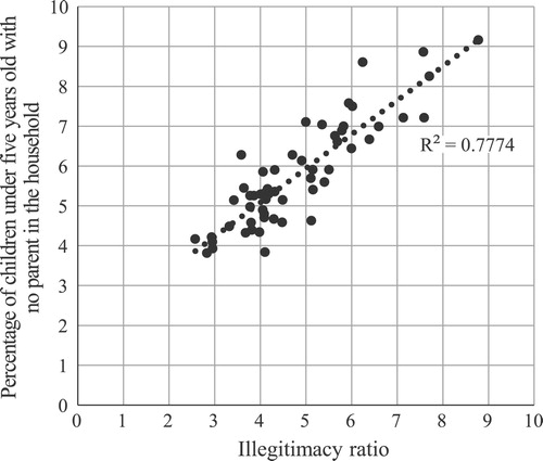
Despite this, the consideration of non-own children is still important, as the possibility that a large proportion of them were illegitimate raises issues for the calculation of marital fertility. It is very difficult to tell whether illegitimate children really did make up a large proportion of non-own children. However, our estimates of the number of illegitimate children born in the five years leading up to 1911 who survived to be enumerated in the Census suggest that up to 61 per cent of unmatched children may have been illegitimate. It is also notable that there is striking similarity in the geographic patterns of the percentage of births that were illegitimate and the percentage of children under age five who were not living with their parents. Figure 3 shows that the correlation between these two variables, at a county level, was high (R² = 0.78).

Figure 3 Relationship between percentage of children aged 0–4 with no parent in the household (1911) and the illegitimacy ratio (1910): counties of England and Wales

Notes: The illegitimacy ratio is the number of illegitimate births as a percentage of all births. Each dot represents a county.

Source: Authors’ calculations based on 1911 Census data from I-CeM and illegitimacy data from the Registrar General’s Annual Report for 1910 (see Appendix for more detail on sources).

Of course we are not arguing that all illegitimate children were non-own (living apart from their mother): we have already mentioned the very small group identified as children of an unmarried mother, and we suspect that there was also a larger group of own children who were illegitimate but whose mothers (incorrectly) reported themselves to be married. Nor are we arguing that all non-own children were illegitimate; there will have been non-own legitimate children as mentioned earlier. Nevertheless, we do argue that illegitimate children made up a large proportion of non-own children, and thus, for the calculation of marital fertility in nineteenth-century England and Wales, non-own children should not be redistributed among married women. We also argue that women who reported themselves as currently married but had no husband in the household were likely to have been unmarried and therefore that including them in marital fertility is misleading. Of course this might not have been the case in all communities: many husbands may have been temporarily absent from fishing villages, port cities, and military bases. In forthcoming papers we will compare versions of marital fertility including these women, and widows, to investigate the effects of spousal separation and widowhood on changes in fertility.

Marital fertility using the OCM

The OCM can be used to calculate marital fertility, but to do this, it is necessary to take duration of marriage, or exposure to the risk of pregnancy, into account. In the past, three variants for doing this have been used.

Variant A: ASFRs multiplied by inverse of proportions married

This variant calculates ASFRs using the standard OCM and then multiplies these by the inverse of the proportion of women married in that age group (Haines 1978, 1979; Retherford and Mirza 1982; Cho et al. 1986). It generally carries the assumption that all fertility occurs within marriage, although some scholars (e.g., Breschi and Serio 2003) adjust for illegitimacy by multiplying by the proportion legitimate as well as dividing by the proportion married. In our comparisons we use ASFRs and proportions married by single year of age.

Variant B: Duration of marriage

This variant takes married women only and uses data on duration of marriage, provided by the census or survey, to calculate the number of women exposed at each age (Cho 1968; Tolnay 1981; Tolnay et al. 1982; Retherford and Cho 1984). Here we use the equation in Box 1 to calculate the number of woman-years of exposure, N_x (see Section 3 of the supplementary material for explanation of the equation).

Box 1. Equation for variant B.

(1) $N_x=\frac{M_x^0}{8}+\frac{M_x^{1-34}}{2}+\frac{M_{x+1}^1}{2}+M_{x+1}^{2-34}+\frac{M_{x+2}^2}{2}+M_{x+2}^{3-34}+\frac{M_{x+3}^3}{2}+M_{x+3}^{4-34}+\frac{M_{x+4}^4}{2}+M_{x+4}^{5-34}+\frac{3M_{x+5}^5}{8}+\frac{M_{x+5}^{6-34}}{2}$(1) where $M_x^i$ is the number of married women aged $x$ with duration of marriage $i$.

Variant C: No adjustment for exposure

This variant uses married woman only and recognizes that back-projecting the number of women married at later ages overestimates exposure to marriage among young women, and therefore underestimates fertility at these ages (Garrett et al. 2001). If children not matched to their mother are adjusted for, this variant also assumes that all fertility occurs within marriage. To avoid having to make this assumption, some researchers consider only currently married women with their spouse present in the household on census night. This carries the alternative assumption that all children living apart from their mothers are the result of unmarried motherhood, orphanhood, or abandonment. Those who follow this route generally consider only children under five years of age, as the assumption becomes less plausible at older ages (Woods and Smith 1983; Hinde and Woods 1984; Garrett et al. 2001).

Issues with variants A, B, and C

Most historical data lack information on duration of marriage, so variant A is the most common variant deployed. It has been used to calculate marital fertility for countries, geographical areas, and also social groups (Breschi, Derosas, et al. 2003; De Santis 2003; Oris 2003; Scalone and Dribe 2012; Gruber and Scholz 2016; Scalone and Dribe 2017). Using this variant to calculate fertility for social groups involves calculating the percentage of women in each social group who were married, and therefore being able to identify the social status of both married and unmarried women. This is highly problematic—at least in the British context—because of the link between women’s occupational status and marital status. Social status or class may be assigned to a woman on the basis of her own occupation, but this is difficult when not all women work, particularly when they are likely to have given up paid work after marriage or childbearing. In such circumstances it is common to use father’s occupation for daughters still living at home and husband’s occupation for wives, but this leaves a gap in societies—such as nineteenth- and early-twentieth-century England and Wales—where women experience a lengthy period during their teens and twenties where they are with neither father nor husband. Women’s own occupations during this period were constrained to certain types of job, such as domestic or agricultural servitude, which in many cases reflected neither the household they came from nor that they would eventually marry into. Neither can occupation of the head of the household in which they were living between leaving home and marriage be used as a proxy, as many women were domestic servants in a wealthier household than that from which they originated or in which they ended up. Certain occupational groups were therefore dominated by single women, but this is not a good guide to the marriage age or duration of any group of married women.

We now present two new variants for calculating marital fertility. The first, variant D, allows relaxation of the assumption that all fertility occurs within marriage, and the second, variant E, also allows the more robust calculation of marital fertility by social group.

Variant D (new): Proportions of women married applied to populations of women

This variant uses married women only and back-projects exposure based on the proportions of women married at each age in the five years leading up to the census. This variant allows non-own children to be treated as illegitimate, and also allows researchers to exclude women (and their children) without their spouse present if this is felt to be appropriate. In our application of this variant, we use children aged 0–4, of married women only, and calculate fertility rates by single years of age. We calculate rates for the five years leading up to the census, so our calculations need to include both children and the exposure contributed by women who had moved to an older age by the time of the census.

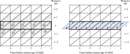
The estimation procedure for age-specific marital fertility rates (ASMFRs) follows a set of computational steps which are explained in Box 2, with numerators and denominators illustrated in Figure 4.

Box 2. Computational steps and equations for variant D.

First, the number of children born to women aged $x$ in the five years before the census, B^x , is estimated. Equation (2) reverse-projects enumerated children to the time of their birth:(2) $C_{0-4}^x=(C_0^x+C_0^{x+1}+C_1^{x+1}+C_1^{x+2}+C_2^{x+2}+C_2^{x+3}+C_3^{x+3}+C_3^{x+4}+C_4^{x+4}+C_4^{x+5})\times 0.5$(2) where $C_a^x$ is the number of children aged $a$ to women aged $x$ in the census. Equation (3) adjusts for mortality:(3) $B^x=\left(\frac{\left(C_0^x+C_0^{x+1}\right)}{{}_1{L}_0}+\frac{\left(C_1^{x+1}+C_1^{x+2}\right)}{{}_1{L}_1}+\frac{\left(C_2^{x+2}+C_2^{x+3}\right)}{{}_1{L}_2}+\frac{\left(C_3^{x+3}+C_3^{x+4}\right)}{{}_1{L}_3}+\frac{\left(C_4^{x+4}+C_4^{x+5}\right)}{{}_1{L}_4}\right)\times 0.5$(3) where ${}_1{L}_a$ values are single-year survivorship probabilities from an appropriate life table. The number of children born in the five years leading up to the census and the years of exposure are illustrated in the Lexis diagrams in Figure 4, where the boxes outlined thickly in black indicate the experience we want to capture. The next step involves estimating woman-years of exposure for women aged$x$, N_x. The equation used in this case is:(4) $N_x=(W_x\times m_x)\times 0.5+(W_{x+1}\times m_x)+(W_{x+2}\times m_x)+(W_{x+3}\times m_x)+(W_{x+4}\times m_x)+(W_{x+5}\times m_x)\times 0.5$(4) where $W_x$ represents the number of women aged $x$ at census year and $m_x$ is the proportion of women aged $x$ who are married at the time of enumeration.

The calculation of ASMFRs for single years or five-year age groups is then straightforward:(5) $\mathrm{A}\mathrm{S}\mathrm{M}\mathrm{F}\mathrm{R}=\frac{B^x}{N_x}\times 1,000.$(5)

Figure 4 Lexis diagrams to illustrate numerators (left) and denominators (right) for the calculation of fertility

Note: See ‘Variant D (new)’ subsection and equations (2)–(4) for explanation of terms.

Variant E (new): Proportions of men married (or standard proportions of women married) applied to populations of women

This variant, which enables the calculation of fertility for social groups based on husbands’ occupations, uses married women with resident husbands only and back-projects exposure based on the relative proportions of men married at each age in the five years leading up to the census, adjusting for the mean spousal age gap.

In this variant the numerator of the ASMFR equation is exactly the same as in variant D. The computational steps and equations for calculating the denominator are shown in Box 3. Essentially, we are adjusting the number of married women aged $x+n$ at the census by the ratio of the proportion married at that age relative to the proportion married at one or more years older. A woman’s marital duration will, by definition, be the same as that of her husband, so if the spousal age gap is relatively constant by age, and if the change in proportions married by age is similar among men and women, then using the ratios of proportions of men married, shifted by the average spousal age gap, should give a similar result. We will consider the plausibility of these assumptions as we discuss the results next.

Box 3. Computational steps and equations for variant E.

In variant E, the woman-years of exposure for women aged $x$, N_x, is estimated by:(6) $N_x=\frac{h_{x+y}}{h_{x+y}}\times M_x\times 0.5+\frac{h_{x+y}}{h_{x+y+1}}\times M_{x+1}+\frac{h_{x+y}}{h_{x+y+2}}\times M_{x+2}+\frac{h_{x+y}}{h_{x+y+3}}\times M_{x+3}+\frac{h_{x+y}}{h_{x+y+4}}\times M_{x+4}+\frac{h_{x+y}}{h_{x+y+5}}\times M_{x+5}\times 0.5$(6) where $M_x$ denotes the number of married women aged $x$ at census year, for $x$ to $x+4$; $h_x$ is the proportion of men aged $x$ who are married at census; and $y$ is the average spousal age gap, rounded to a whole number (note that in the first term $h_{x+y}/h_{x+y}$ cancels out). The rationale for this is as follows. In variant D each cell of exposure is:(7) $(W_{x+n}\times m_x)\mathrm{o}\mathrm{r}{W}_{x+n}\times \frac{M_x}{W_x}\mathrm{o}\mathrm{r}\frac{W_{x+n}\times M_x}{W_x}$(7) where, as before, $W_x$ represents the number of women aged $x$ at census year, M_x is the number of married women aged x at census year, and $m_x$ is the proportion of women aged $x$ who are married at the time of enumeration.

Multiplying this through by the number of married women ($M_{x+n}$) gives:(8) $\frac{W_{x+n}\times M_x\times M_{x+n}}{W_x\times M_{x+n}}\mathrm{o}\mathrm{r}\frac{W_{x+n}\times M_x}{W_x\times M_{x+n}}\times M_{x+n}$(8) which can be rewritten as:(9) $\frac{M_x/W_x}{M_{x+n}/W_{x+n}}\times M_{x+n}\mathrm{o}\mathrm{r}\frac{m_x}{m_{x+n}}\times M_{x+n}.$(9)

Comparing variants for calculating marital fertility

For England and Wales

Figure 5 shows the ASMFRs (for women aged 20–49) for England and Wales in 1911, calculated using the five variants of the OCM laid out in the previous section, and Table 3 summarizes these in terms of total marital fertility rates (TMFRs). Two versions of TMFR are shown in Table 3: TMFR₂₀ shows the number of children a woman would have had if she had married at age 20 and experienced the ASMFRs for each age in turn, while TMFR₂₅ shows the number of children she would have had if she had married at age 25.

Figure 5 Age-specific marital fertility rates (ASMFRs) calculated using five different variants of the OCM: England and Wales, 1911

Note: See ‘Marital fertility using the OCM’ section for details of variants.

Source: Authors’ calculations based on 1911 Census data from I-CeM and mortality data from the Human Mortality Database (see Appendix for more detail on sources).

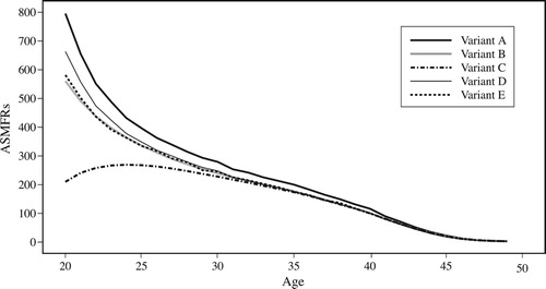
Table 3 Total marital fertility for women marrying at age 20 (TMFR₂₀) and age 25 (TMFR₂₅), England and Wales, 1911, calculated using five different variants of the OCM

	TMFR20	TMFR25
Variant A	7.09	4.16
Variant B	5.89	3.64
Variant C	4.65	3.40
Variant D	6.17	3.68
Variant E	5.93	3.65

Note: See ‘Marital fertility using the OCM’ section for details of variants.

Source: Authors’ calculations based on 1911 Census data from I-CeM and mortality data from the Human Mortality Database (see Appendix for more detail on sources).

Variant A produces the highest fertility. This variant is often used with five-year age groups, but when it is used with single years of age, it differs from variant D primarily in the fact that the numerator for variant A includes non-own children. Not unsurprisingly, assuming all children are legitimate results in a higher estimation of marital fertility, but the effect is not very large. Variant C consistently gives the lowest fertility, showing implausibly low fertility among young married women. This is attributable to the lack of adjustment for marital duration: in essence the variant assumes married women had been married for the full five years before the census. Therefore, we strongly urge against using variant C.

It is worth remembering that the numbers of children used for variants B, C, D, and E are exactly the same; therefore, the differences between the results are due entirely to differences in calculated exposure. Differences in exposure are small, with estimates from variant D giving slightly higher exposure for older women and slightly lower exposure for younger women. Because the number of married women is high at older ages, differences in exposure make very little difference to fertility. However relatively low numbers of married women in their early twenties mean that small differences in exposure can produce large differences in fertility. Therefore, these variants result in very similar fertility among women over the age of 30, but greater discrepancy among women in their early twenties, resulting in noticeable differences in TMFR₂₀ (5.89, 6.17, and 5.93 using variants B, D, and E, respectively), although differences in TMFR₂₅ are minimal (3.64, 3.68, and 3.65, respectively). Before considering how these variants perform in situations with different marriage patterns, it is worth considering why they produce different results.

As noted earlier in the ‘Data’ section, the preceding comparisons have all (except variant A) been carried out using only those married women in 1911 who gave consistent age, duration of marriage, and fertility information and who could be linked to a husband in the same household. This selection was used in order to allow comparisons of the different variants, but calculations of proportions married (for variants A, D, and E) need to use both married and unmarried women, as the exclusion of the 18.5 per cent of married women who gave inconsistent information or whose husband was not in the household would alter the proportions. Systematic differences in durations married between married women excluded from and included in the data set may have affected the calculations. It is important, therefore, to consider whether women giving inconsistent fertility or marital duration information in 1911 were an unbiased subset of the married population.

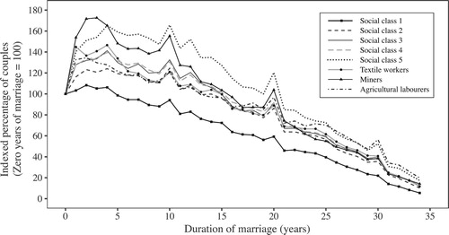
Figure 6 shows the distribution of marital durations across couples with consistent information in 1911. Unsurprisingly there is heaping at durations of ten and 20 years, but the most noticeable feature is a deficit of couples with very short marital durations, particularly zero years. While it is possible this could have been produced by a sudden drop in marriages in the years leading up to 1911, the number of marriages registered in England and Wales was actually slightly higher in 1908–10 than it had been in previous years (Office for National Statistics 2019). The deficit of couples reported as recently married in the 1911 Census was also noticed by Thomas Stevenson, who compiled the official reports on fertility arising from the 1911 Census. He argued that this was partly due to couples ‘accidentally’ reporting the duration at the next wedding anniversary rather than at the previous one (1911 Census of England and Wales 1923, pp. viii–x). Stevenson did not discuss why couples may have given such ‘accidental’ responses, beyond stating that he expected it to be more likely among less educated couples. We speculate that some couples may have worked out their marital duration from the age of their oldest child, or by subtracting 1911 from the year of their marriage. Figure 7, showing the distribution of couples giving particular marital durations by social class, indexed against zero years, demonstrates that the deficit was indeed strongest among the manual and unskilled social classes. Stevenson also noted that the deficit in marriages of less than one year was particularly acute among those with young ages at marriage, who were also most likely to have been pregnant on marriage, and he argued that such couples were systematically overstating their marital duration to hide a premarital conception (1911 Census of England and Wales 1923, pp. viii–x).

Figure 6 Number of couples by duration of marriage: England and Wales, 1911

Source: As for Figure 1.

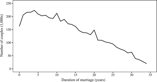
Figure 7 Distributions of couples by duration of marriage (in years), indexed at zero years married, by social class: England and Wales, 1911

Note: Social classes 1–5 include occupational groups as follows: 1: professional occupations; 2: skilled non-manual occupations; 3: skilled manual occupations; 4: semi-skilled manual occupations; 5: unskilled manual occupations.

Source: As for Figure 1.

The systematic overstatement of marital duration could explain why variant B gives lower fertility estimates than most of the other variants. However, we should also consider whether the deficit of short marital durations could be the result of missing data. The Census instructions stated that marital duration and fertility information were to be filled out for married women, but it was not uncommon for a man to have entered the information against his own rather than his wife’s name. In such cases the Census clerks would strike this out and rewrite the information in the row for the wife. However, in so doing they would sometimes use ‘–’ to indicate a zero. The transcriptions do not include the crossed-out records and so it is impossible to tell whether the ‘–’ indicates a real missing entry (e.g., if they were not married or did not know their marital duration) or a checking clerk’s zero. If the absence of very short marital durations is because they were omitted, rather than because marital durations were overstated, then fertility calculated by variant B will be correct for those included in the selection, but exposures calculated using variant D will overestimate the durations of marriage and therefore underestimate fertility. This recording practice might have been more likely among less educated couples, but it should also have been more likely among the young, where short marital durations were concentrated. However, although very young women were particularly likely to have been missing a marital duration (perhaps due to some unmarried mothers reporting themselves as married), the proportion missing a marital duration increased steadily from about age 25. Overall, therefore, it is likely that the deficit of people married for less than a year was due more to overstatement of marital durations, leading to understatement of fertility in variant B, but this may have been partially offset by omission of some of those married for less than a year.

For England and Wales as a whole, variant E gives slightly lower fertility than variant D, particularly among younger women. This is due to the fact that the marriage curve for men is slightly steeper than that for women, so the area under the curve for a five-year age span is larger than that for women. However, differences are small at the national level.

For types of place

We developed variant E for use with social groups where it is not possible to calculate proportions of married women, and our first tests compare variants D and E within places characterized by very different marriage patterns for men and women. Figure 8 shows the ASMFRs for the three selected types of place using the five different variants, while Table 4 shows the corresponding values of TMFR₂₀ and TMFR₂₅. Table 4 also shows variant ‘E.std’, which uses a standard marriage schedule for females (here, that for all England and Wales in 1911) instead of the marriage schedule for men for the type of place.

Figure 8 Age-specific marital fertility rates (ASMFRs) calculated using different variants of the OCM: professional, mining, and textile places within England and Wales, 1911

Note: See ‘Marital fertility using the OCM’ section for details of variants.

Source: Authors’ calculations based on 1911 Census data from I-CeM and mortality data from the Human Mortality Database and the Quarterly Reports of the Registrar General of England and Wales (see Appendix for more detail on sources).

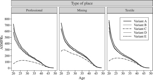
Table 4 Total marital fertility for women marrying at age 20 (TMFR₂₀) and age 25 (TMFR₂₅), by type of place in England and Wales, 1911, calculated using six different variants of the OCM

	Type of place			E&W
	Mining	Professional	Textile
TMFR20
Variant A	7.47	6.31	6.12	7.09
Variant B	6.88	5.57	5.42	5.89
Variant C	4.80	2.25	2.98	4.65
Variant D	6.77	5.79	5.41	6.17
Variant E	6.82	5.42	5.47	5.93
Variant E.std	7.35	5.33	5.20	5.93
TMFR25
Variant A	4.67	3.60	3.46	4.16
Variant B	4.38	3.29	3.17	3.64
Variant C	3.37	1.76	2.27	3.40
Variant D	4.26	3.32	3.11	3.68
Variant E	4.34	3.22	3.10	3.65
Variant E.std	4.40	3.17	3.09	3.65

Note: See ‘Marital fertility using the OCM’ section and ‘Comparing variants for calculating marital fertility’ section (‘For types of place’ subsection) for details of variants.

Source: As for Table 1.

Table 4 shows that differences in estimated fertility between the different variants for places with extreme marriage patterns are larger than those for England and Wales as a whole. Variant C shows particularly large understatement for professional areas, where marriage was late, because the overestimation of exposure is more severe, and this is also clearly seen in Figure 8. For England and Wales as a whole, variant E gives slightly lower fertility estimates than variant D, and this pattern is exacerbated in professional areas where the marriage curve for men is steeper than that of women. In places where women married young relative to men, such as mining areas, the marriage pattern for men is less steep than for women and variant E generates slightly higher fertility. In general, however, it seems that different marriage patterns in different places do not make much difference to estimates of fertility, particularly for TMFR₂₅. Our final comparison for different types of place tests this by using the same marriage pattern (here, that for all England and Wales in 1911) for all types of place. Results, however, show that the marriage patterns for men (variant E) for particular types of place represent their respective patterns for women better than a standard marriage pattern (variant E.std) does. Section 4 of the supplementary material demonstrates that a further variation, which excludes servants from the marital fertility calculations, significantly underestimates fertility in places where servant-keeping was common.

This subsection has tested variants of the OCM for estimating marital fertility for different types of place with different marriage patterns, to allow comparison of variants D and E, which use proportions of women and men married, respectively, to estimate exposure. The marriage patterns in these places were driven by the behaviour of particular social groups—the middle classes in professional areas and miners in mining areas. Yet these social groups were still generally a minority or a small majority in the places they typify, and their marriage behaviour was likely to be more extreme. The next section therefore compares variants B and E for different social classes.

For social classes

Figure 9 shows ASMFRs for social classes using variants B, E, and E.std, while Table 5 shows the corresponding values of TMFR₂₀ and TMFR₂₅. In general, variant E generates lower fertility compared with variant B (which we have already established is likely to underestimate fertility a little). The deficit in TMFR₂₀ is between 0.37 and 0.93 children per woman, but this is concentrated among younger women, so the deficit in TMFR₂₅ (0.18–0.28 children per woman) is both smaller and less variable. The differences between variants B and E are largest for social classes ‘1’ and ‘2’ (professional and non-manual occupations), and also for agricultural labourers, as spousal age gaps in these groups are larger. Variant E.std results differ less from variant B at young ages for social class ‘2’ and for agricultural labourers, but results for social class ‘1’ are just as low as for variant E, and results for social class ‘5’ (unskilled manual workers) and miners, whose wives married at younger ages than the national average, are considerably higher.

Figure 9 Age-specific marital fertility rates (ASMFRs) calculated using three different OCM variants, for different social classes: England and Wales, 1911

Note: See ‘Marital fertility using the OCM’ section for details of variants.

Source: As for Figure 8.

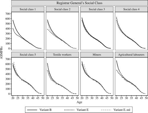
Table 5 Total marital fertility for women marrying at age 20 (TMFR₂₀) and age 25 (TMFR₂₅), by social class in England and Wales, 1911, calculated using three different variants of the OCM

	Variant B	Variant E	Variant E.std
TMFR20
Social class 1	5.33	4.41	4.41
Social class 2	5.81	4.95	5.36
Social class 3	6.21	5.82	5.99
Social class 4	6.30	5.89	6.11
Social class 5	6.85	6.48	7.11
Textile workers	5.43	4.83	5.15
Miners	7.51	7.13	7.95
Agricultural labourers	7.09	6.34	6.98
TMFR25
Social class 1	3.05	2.77	2.77
Social class 2	3.47	3.19	3.24
Social class 3	3.75	3.56	3.60
Social class 4	3.84	3.65	3.66
Social class 5	4.38	4.17	4.24
Textile workers	3.17	2.99	3.03
Miners	4.91	4.70	4.83
Agricultural labourers	4.47	4.20	4.25

Notes: See ‘Marital fertility using the OCM’ section and ‘Comparing variants for calculating marital fertility’ section (‘For types of place’ subsection) for details of variants. Social classes 1–5 include occupational groups as follows: 1: professional occupations; 2: skilled non-manual occupations; 3: skilled manual occupations; 4: semi-skilled manual occupations; 5: unskilled manual occupations.

Source: As for Table 1.

Conclusions

This paper has presented two new variants of the OCM for calculating marital fertility, which calculate exposure to marriage by adjusting the numbers of married women using ratios of the proportions of women and men married. We compared the results from these new variants against the results obtained using older variants of OCM, including the variant that uses exposure calculated from reported durations of marriage. We tested them using big data from the whole of England and Wales in 1911, for specific types of place with different marriage regimes, and also for social groups.

We argue that there is good reason to think that durations of marriage are slightly over-reported and therefore fertility rates calculated using durations married to generate exposure are likely to be a little too low, an effect also found in similar comparisons elsewhere (Tolnay et al. 1982). However, it is worth bearing in mind that inflation of marital duration in order to disguise a prenuptial pregnancy or illegitimate child may actually be a better indicator than actual marital duration of exposure to the risk of pregnancy. It has been estimated that around half of all first births in 1800 in Britain were either illegitimate or conceived prenuptially (Levene et al. 2005, p. 6). Illegitimacy dropped over the course of the nineteenth century, and it is plausible that there was a concomitant increase in prenuptial pregnancy. The marital fertility rates of young women were likely to have been pushed upwards by both underestimated exposure and high fecundity, with those who fell pregnant selected into marriage.

Our new variants of the OCM, which use ratios of the proportions of women or men married in successive age groups, all generate substantially similar ASFRs, particularly for ages over 25, suggesting that the calculation of exposure to marriage using proportions married is not particularly sensitive to marriage patterns. This insensitivity to marriage patterns is perhaps surprising, given the large differences between men and women in proportions married, but this can be explained by the fact that only five years’ worth of exposure is being considered. The variant adjusts the number of married women of a particular age by the ratio of proportions of men married at the same age (adjusted for the spousal age gap) to the proportions married at one, two, three, or four years older. These ratios will become increasingly different to the equivalent ratios for women as the number of years increases, but each of these years only contributes a small amount to the overall calculation. In general, using the proportions of men married produces slightly lower estimates of fertility, particularly at young ages. These are likely to be underestimates because the marriage curve for men tends to be slightly steeper than that of women, and are exacerbated where there are larger differences in the marriage patterns of men and women, particularly among the higher social groups. Nevertheless, we feel that it is reasonable to use ratios of proportions of men married when calculating fertility for social groups. If desired, a standard marriage schedule for women may be used instead, but our findings indicate that this increases the range of the discrepancies.

The TMFR is a very strange beast. Unlike many demographic measures—even those calculated from synthetic cohorts or cross-sectional surveys (such as SMAM)—and unlike the TFR, it cannot be thought of as capturing the experience of a ‘typical’ woman. Instead, it measures the fertility of a hypothetical woman who married at a particular age. This is usually 15, but here we have used 20 or 25, and we argue that TMFR₂₅ is preferable for comparing subgroups in England and Wales. Even in societies with relatively complete and early marriage for women, the TMFR often indicates implausibly high fertility (Hoem and Mureşan 2011) and this is particularly the case in societies with late marriage, such as England and Wales. In 1911 the SMAM was 26.2 for women and 27.6 for men, and only 7 per cent of 20-year-old women were already married. In this society, where premarital sexual intercourse and conception were common, the ASMFRs for those who married in their teens and early twenties are inflated by selection of the already pregnant into marriage (see also Wrigley et al. 1997, pp. 378–9). Rates for young married women are also quite susceptible to variations in proxy marriage patterns used when it is not possible to calculate proportions married, for example for social classes, and this is another reason for recommending TMFR₂₅ as the preferred summary measure of marital fertility in historical populations.

In summary, we have presented two new variants of the OCM—dubbed variant D and variant E—for the calculation of age-specific marital fertility. These provide two distinct advantages over the standard variants of the OCM for calculating marital fertility. Both variants allow relaxation of the assumption that all children are legitimate, and the second also allows the more accurate calculation of marital fertility for social groups when reported durations of marriage are unavailable. We have tested them extensively and demonstrated that they work well, despite some underestimation among late-marrying social groups. There has been a recent and continuing growth in the availability of full-count census data for historical populations, opening up possibilities for the comparison of age-specific fertility (both within marriage and overall) for population subgroups. Our new variants of the OCM will facilitate and improve such comparisons and will therefore produce more nuanced analyses of historical trends in fertility during the first demographic transition1 2 3 4.

Notes

1 Please direct all correspondence to Alice Reid, Cambridge Group for the History of Population and Social Structure, Department of Geography, University of Cambridge, Downing Place, Cambridge CB2 3EN, UK; or by E-mail: [email protected]; Twitter: @amrcampop

2 Alice Reid is based at the Cambridge Group for the History of Population and Social Structure, Department of Geography, University of Cambridge. Hannaliis Jaadla is also based at the Cambridge Group for the History of Population and Social Structure, as well as the Estonian Institute for Population Studies, Tallinn University. Eilidh Garrett was based at the Department of History, University of Essex, when this research was carried out. Kevin Schürer is based at the Centre for English Local History, University of Leicester.

3 This work was supported by the Economic and Social Research Council under Grant ES/L015463/1.

4 We are very grateful to George Alter for patiently listening to us work through these variants over coffee in the Cambridge Group.

Appendix:

Data sources

This work is based on I-CeM, a standardized, integrated data set of most of the censuses of Great Britain for the period 1851–1911; see K. Schürer and E. Higgs, Integrated Census Microdata (I-CeM); 1851–1911 [computer file]. Colchester, Essex: UK Data Archive [distributor], April 2014. SN: 7481, https://doi.org/10.5255/UKDA-SN-7481-1. A user guide and manual to the I-CeM data is available at E. Higgs, C. Jones, K. Schürer, and A. Wilkinson, The Integrated Census Microdata (I-CeM) Guide (Colchester, 2013). Further details on the I-CeM database, together with a number of related resources, are available from the I-CeM website at: https://www1.essex.ac.uk/history/research/icem/

The creation of the I-CeM database was made possible through funding from the UK Economic and Social Research Council (ESRC), grant number RES-062–23–1629. The version of the I-CeM data used here has been enhanced as a result of work by K. Schürer, H. Jaadla, A. Reid, and E. Garrett as part of the ESRC-funded ‘An Atlas of Victorian Fertility Decline’ project (ES/L015463/1) at the Cambridge Group for the History of Population and Social Structure, Department of Geography, University of Cambridge, and will be deposited with the UK Data Archive at a future date. For further details, see http://www.geog.cam.ac.uk/research/projects/victorianfertilitydecline/

Mortality data for England and Wales were obtained from the Human Mortality Database at: http://www.mortality.org/, from the Decennial Reports of the Registrar General of England and Wales (R. I. Woods, Causes of Death in England and Wales, 1851–60 to 1891–1900: The Decennial Supplements, UKDA SN3552, doi.org/10.5255/UKDA-SN-3552-1), and from our own transcriptions of the Quarterly Reports of the Registrar General of England and Wales.

References

- 1911 Census of England and Wales. 1923. Volume XIII: Fertility of Marriage Part 2. London: HMSO.
- Abbasi-Shavazi, M. J. 1997. An assessment of the own-child method of estimating by birthplace in Australia, Journal of the Australian Population Association 14(2): 167–185. doi: 10.1007/BF03029338
- Adair, R. 1996. Courtship, Illegitimacy and Marriage in Early Modern England. Manchester: Manchester University Press.
- Avery, C., T. St Clair, M. Levin, and K. Hill. 2013. The ‘own children’ fertility estimation procedure: A reappraisal, Population Studies 67(2): 171–183. doi: 10.1080/00324728.2013.769616
- Boot, H. M. 2017. Using census returns and the own-children method to measure marital fertility in Rawtenstall, 1851–1901, Local Population Studies 98: 54–73. doi: 10.35488/lps98.2017.54
- Breschi, M. and N. Serio. 2003. Fertility at the time of the 1427 Florentine Catasto, in M. Breschi, S. Kurosu, and M. Oris (eds), The Own-Children Method of Fertility Estimation. Applications in Historical Demography. Udine: Forum, pp. 27–52.
- Breschi, M., R. Derosas, and R. Rettaroli. 2003. Fertility and socio-economic status in nineteenth-century urban Italy, in M. Breschi, S. Kurosu, and M. Oris. (eds), The Own-Children Method of Fertility Estimation. Applications in Historical Demography. Udine: Forum, pp. 101–123.
- Breschi, M., S. Kurosu, and M. Oris. 2003. The Own-Children Method of Fertility Estimation. Applications in Historical Demography. Udine: Forum.
- Childs, G. 2004. Demographic analysis of small populations using the own-children method, Field Methods 16(4):379–395. doi: 10.1177/1525822X04269172
- Cho, L. J. 1968. Income and differentials in current fertility, Demography 5(1): 198–211. doi: 10.1007/BF03208572
- Cho, L. J. 1974. The own-children approach to fertility estimation: An elaboration, International Population Conference Liege 1973, 2: 263–279.
- Cho, L. J., R. D. Retherford, and M. K. Choe. 1986. The Own Children Method of Fertility Estimation. Honolulu: University of Hawaii Press for the Population Institute, East-West Population Center.
- Coleman, D. A. and S. Dubuc. 2010. The fertility of ethnic minorities in the UK, 1960s–2006, Population Studies 64(1): 19–41. doi: 10.1080/00324720903391201
- De Santis, G. 2003. The own-children method of fertility estimation in historical demography: A glance backward and a step forward, in M. Breschi, S. Kurosu, and M. Oris (eds), The Own-Children Method of Fertility Estimation. Applications in Historical Demography. Udine: Forum, pp. 11–26.
- Dribe, M. and F. Scalone. 2014. Social class and net fertility before, during and after the demographic transition: A micro-level analysis of Sweden 1880–1970, Demographic Research 30(15): 429–464. doi: 10.4054/DemRes.2014.30.15
- Dribe, M, S. P. Juarez, and F. Scalone. 2017. Is it who you are or where you live? Community effects on net fertility during the demographic transition in Sweden: A multilevel analysis using micro-census data, Population, Space and Place 23: e1987. doi: 10.1002/psp.1987
- Dubuc, S. 2009. Application of the own-children method for estimating fertility by ethnic and religious groups in the UK, Journal of Population Research 26: 207–225 doi: 10.1007/s12546-009-9020-7
- East–West Center. 1992. EASWESPOP—Fertility Estimate Programs: User’s Manual version 2.0. Available: http://www.eastwestcenter.org/fileadmin/resources/research/PDFs/manual_fertility_estimate.pdf last (accessed: 6 April 2017).
- Garrett, E. M., A. M. Reid, K. Schürer, and S. Szreter. 2001. Changing Family Size in England and Wales: Place, Class and Demography, 1891–1911. Cambridge: Cambridge University Press.
- Goldstein, S. and A. Goldstein. 1981. The impact of migration on fertility: An ‘own children’ analysis for Thailand, Population Studies 35(2): 265–284.
- Grabill, W. H. and L. J. Cho. 1965. Methodology for the measurement of current fertility from population data in young children, Demography 2: 50–73. doi: 10.2307/2060106
- Gruber, S. and R. Scholz. 2016. Fertility in Rostock in the 19th century, MPIDR Working Paper 2016-001.
- Hacker, J. D. 2003. Rethinking the ‘early’ decline of marital fertility in the United States, Demography 40(4): 605–620. doi: 10.1353/dem.2003.0035
- Hacker, J. D. 2016. Ready, willing, and able? Impediments to the onset of marital fertility decline in the United States, Demography 53(6): 1657–1692. doi: 10.1007/s13524-016-0513-7
- Haines, M. R. 1978. Fertility decline in industrial America: An analysis of the Pennsylvania anthracite region, 1850–1900, using ‘own children’ methods, Population Studies 32(2): 327–354.
- Haines, M. R. 1979. Fertility and Occupation: Population Patterns in Industrialization. New York: Academic Press.
- Haines, M. R. 1989. American fertility in transition: New estimates of birth rates in the United States, 1900–1910, Demography 26(1): 137–148. doi: 10.2307/2061500
- Hareven, T. K. and M. A. Vinovskis. 1975. Marital fertility, ethnicity, and occupation in urban families: An analysis of South Boston and the South End in 1880, Journal of Social History 8(3): 69–93. doi: 10.1353/jsh/8.3.69
- Higgs, Edward. 2004. Life, death and statistics: Civil registration, censuses and the work of the General Register Office, 1836–1952, Hatfield: Local Population Studies.
- Hinde, Andrew. 2003. England’s Population: A History Since the Domesday Survey. London: Edward Arnold.
- Hinde, P. R. A. and R. I. Woods. 1984. Variations in historical natural fertility patterns and the measurement of fertility control, Journal of Biosocial Science 16: 309–321. doi: 10.1017/S0021932000015133
- Hoem, J. M. and C. Mureşan. 2011. The total marital fertility rate and its extensions, European Journal of Population 27: 295–312. doi: 10.1007/s10680-011-9237-y
- Jaadla, H. and A. M. Reid. 2017. The geography of early childhood mortality in England and Wales, 1881–1911, Demographic Research 37: 1861–1890. doi: 10.4054/DemRes.2017.37.58
- Klüsener, S., M. Dribe, and F. Scalone. 2016. Spatial and social distance in the fertility transition: Sweden 1880–1900, MPIDR Working paper 2016-009.
- Krapf, S. and M. Kreyenfeld. 2015. Fertility assessment with the own-children method: A validation with data from the German Mikrozensus, MPIDR Technical Report 2015-003.
- Kurosu, S. 2003. Marriage, fertility and economic correlates in nineteenth-century Japan, in M. Breschi, S. Kurosu, M. Oris (eds), The Own-Children Method of Fertility Estimation. Applications in Historical Demography. Udine: Forum. pp. 52–76.
- Laslett, P. and K. Oosterveen. 1973. Long-term trends in bastardy in England: A study of the illegitimacy figures in the parish registers and in the reports of the Registrar-General, 1561–1960, Population Studies 27(2): 255–286.
- Lee, R. and D. Lam. 1983. Age distribution adjustments for English censuses, 1821 to 1931, Population Studies 37(3): 445–464.
- Levene, Alysa, Thomas Nutt, and Samantha Williams. 2005. Introduction, in Alysa Levene, Thomas Nutt, and Samantha Williams (eds), Illegitimacy in Britain, 1700–1920. Basingstoke: Palgrave Macmillan, pp. 1–17.
- Muir, A. J. 2018 Courtship, sex and poverty: Illegitimacy in eighteenth-century Wales, Social History 43(1): 56–80. doi: 10.1080/03071022.2018.1394000
- Myers, R. J. 1993. Errors and bias in the reporting of ages in census data, in Donald J. Bogue, Eduardo E. Arriaga, Douglas L. Anderton, and George W. Rumsey (eds), Readings in Population Research Methodology. Volume 1. Chicago, Illinois: Social Development Center, pp. 4-23–4-29.
- Office for National Statistics. 2019. Marriages in England and Wales, 2016. Available: https://www.ons.gov.uk/peoplepopulationandcommunity/birthsdeathsandmarriages/marriagecohabitationandcivilpartnerships/datasets/marriagesinenglandandwales2013 (accessed: 5 April 2019).
- Oris, M. 2003. The own-children method applied to a rapidly growing industrial population: Coping with the discrepancies between cross-sectional and longitudinal demography, in M. Breschi, S. Kurosu, and M. Oris (eds), The Own-Children Method of Fertility Estimation. Applications in Historical Demography. Udine: Forum, pp. 77–100.
- Reid, A. M., S. J. Arulanantham, J. Day, E. M. Garrett, H. Jaadla, and M. Lucas-Smith. 2018. Populations Past: Atlas of Victorian and Edwardian Population. Available: https://www.populationspast.org/ (accessed: 17 May 2019).
- Retherford, R. D. and I. Alam. 1985. Comparison of fertility trends estimated alternatively from birth histories and own children, Papers of the East-West Population Institute Number 94.
- Retherford, R. D. and L. J. Cho. 1978. Age-parity-specific birth rates and birth probabilities from census or survey data on own children, Population Studies 32(3): 567–581. doi: 10.1080/00324728.1978.10412816
- Retherford, R. D. and L. J. Cho. 1984. Census-derived estimates of fertility by duration since first marriage in the Republic of Korea, Demography 21(4): 537–558. doi: 10.2307/2060914
- Retherford, R. D. and G. M. Mirza. 1982. Evidence of age exaggeration in demographic estimates for Pakistan, Population Studies 36(2): 257–270. doi: 10.1080/00324728.1982.10409031
- Retherford, R. D., A. Chamratrithirong, and A. Wanglee. 1980. The impact of alternative mortality assumptions on own-children estimates of fertility for Thailand, Asian Pacific Census Forum 6(3): 5–8.
- Rindfuss, R. R. 1976. Annual fertility rates from census data on own children: Comparisons with vital statistics data for the United States, Demography 13(2): 235–249. doi: 10.2307/2060803
- Rindfuss, R. R. 1977. Methodological difficulties encountered in using own-children data: Illustrations from the United States, Papers of the East-West Population Institute Number 42.
- Ruggles, S. 2014. Big microdata for population research, Demography 51(1): 287–297. doi: 10.1007/s13524-013-0240-2
- Scalone, F. and M. Dribe. 2012. Socioeconomic status and net fertility in the demographic transition: Sweden in 1900 – a preliminary analysis, Popolazione e Storia 2010(2): 111–132.
- Scalone, F. and M. Dribe. 2017. Testing child-woman ratios and the own-children method on the 1900 Swedish census: Examples of indirect fertility estimates by socioeconomic status in a historical population, Historical Methods 50(1): 16–29. doi: 10.1080/01615440.2016.1219687
- Schoumaker, B. 2017. Measuring male fertility rates in developing countries with Demographic and Health Surveys: An assessment of three methods, Demographic Research 36(28): 803–850. doi: 10.4054/DemRes.2017.36.28
- Schürer, K. 1989. A note concerning the calculation of the singulate mean age at marriage, Local Population Studies 43: 67–70.
- Schürer, K. and E. Higgs. 2014. Integrated Census Microdata (I-CeM); 1851–1911 [computer file]. Colchester, Essex: UK Data Archive [distributor], April 2014. SN: 7481. Available: http://dx.doi.org/10.5255/UKDA-SN-7481-1.
- Schürer, K., E. Garrett, H. Jaadla, and A. Reid. 2018. Household and family structure in England and Wales, 1851–1911: Continuities and change, Continuity and Change 33(3): 365–411. doi: 10.1017/S0268416018000243
- Spoorenberg, T. 2014. Reverse survival method of fertility estimation: An evaluation, Demographic Research 31(9): 217–246. doi: 10.4054/DemRes.2014.31.9
- Tolnay, S. E. 1981. Trends in total and marital fertility for black Americans, 1886–1899, Demography 18(4): 443–463. doi: 10.2307/2060942
- Tolnay, S. E. and A. M. Guest. 1984. American family building strategies in 1900: Stopping or spacing, Demography 21(1): 9–18. doi: 10.2307/2061023
- Tolnay, S. E., S. N. Graham, and A. M. Guest. 1982. Own-child estimates of US white fertility, 1886–99, Historical Methods 15(3): 127–138. doi: 10.1080/01615440.1982.10594087
- United Nations. 1983. Manual X: Indirect Techniques for Demographic Estimation. New York: United Nations.
- Woods, R. and C. W. Smith. 1983. The decline of marital fertility in the late nineteenth century: The case of England and Wales, Population Studies 37(2): 207–225. doi: 10.1080/00324728.1983.10408747
- Wrigley, E. A., R. S. Davies, J. E. Oeppen, and R. S. Schofield. 1997. English Population History from Family Reconstitution 1580–1837. Cambridge: Cambridge University Press.
- Young, C. M. 1992. Australia’s heterogeneous immigrant population: A review of demographic and socioeconomic characteristics, in J. Donovan, E. D’Espaignet, C. Merton, and Van Ommeren (eds), Immigrants in Australia: A Health Profile. Canberra: Australian Government Publishing Service, pp. 11–33.