Cross-sectional average length of life by parity: Country comparisons

Abstract

This study aims to present an alternative measure of fertility—cross-sectional average length of life by parity (CALP)—which: (1) is a period fertility indicator using all available cohort information; (2) captures the dynamics of parity transitions; and (3) links information on fertility quantum and timing together as part of a single phenomenon. Using data from the Human Fertility Database, we calculate CALP for 12 countries in the Global North. Our results show that women spend the longest time at parity zero on average, and in countries where women spend comparatively longer time at parity zero, they spend fewer years at parities one and two. The analysis is extended by decomposing the differences in CALPs between Sweden and the United States, revealing age- and cohort-specific contributions to population-level differences in parity-specific fertility patterns. The decomposition illustrates how high teenage fertility in the United States dominates the differences between these two countries in the time spent at different parities.

Keywords:

• fertility by parity
• multistate life table
• decomposition
• fertility measurement
• cohort analysis
• period analysis

Introduction

Various indicators are typically used in demographic research with the aim of measuring either the quantum or timing of fertility. For instance, the period total fertility rate (TFR) is the demographic statistic most widely used to measure fertility quantum; it is defined as the average number of births a woman would have if she were to live through her reproductive years experiencing the same probabilities of bearing children at each age as those observed in a cross-sectional synthetic cohort of women in a particular year (Preston et al. 2001). In turn, the mean age at childbearing (MAC) provides a measure of fertility timing, and it corresponds to the mean age of mothers at the birth of their children in a specific year. There are also well-known measures that aim to control for the effect of changing fertility timing on the TFR (Ryder 1964), for example the tempo-adjusted TFR (Bongaarts and Feeney 1998; Kohler and Ortega 2002; Schoen 2004; Bongaarts and Sobotka 2012).

From a cohort perspective, there is a clear link between childbearing timing and quantum in advanced societies: compared with earlier starters, women who postpone childbearing typically have fewer children on average and a higher chance of remaining permanently childless (Morgan and Rindfuss 1999; Tomkinson 2019). In fact, the tendency towards the delay of first births implies that less time is left for higher-order birth transitions, increasing the probability of lower completed fertility (Frejka and Sardon 2006). At the aggregate level, the strength of the relationship between timing and quantum is crucial for the overall level of fertility (Frejka and Sobotka 2008; Schmidt et al. 2012). As such, the timing of births affects the parity distribution of specific age groups at a particular point in time, but it can also have long-lasting effects on the propensity to transition to higher parities and the eventual number of children born to (real) cohorts of women.

Period and cohort fertility indicators each have acknowledged strengths and limitations. Whereas the period perspective, based on the synthetic cohort approach, is informative of current fertility levels, it does not necessarily reflect the experience of any cohort of women, particularly during times of changing fertility behaviour (Luy 2011; Bongaarts and Sobotka 2012). Cohort measures, in turn, are based on information on populations that have reached the end of their reproductive years, and they describe fertility behaviour that has taken place several years or even decades earlier. Although both these types of indicators have undoubtedly strengthened our understanding of quantum and timing changes in fertility, in our view, a comprehensive indicator to measure women’s fertile life histories, combining aspects of quantum and timing, as well as period and cohort, would also be useful.

This study aims to present country comparisons based on an alternative indicator to study fertility: the cross-sectional average length of life by parity (CALP). This measure uses the entire age- and cohort-specific information available from birth histories of female cohorts of reproductive age alive at a given time. The concept of CALP builds directly on an existing index developed in mortality research as an alternative measure to life expectancy, namely the cross-sectional average length of life (CAL) (Brouard 1986; Guillot 2003). Recently, the same concept was introduced in fertility research for the transition from parity zero to parity one, to analyse the cross-sectional average length of life childless (CALC) (Mogi et al. 2021) and for the parity transitions from parity zero to parities five and higher with an application to the United States (US) by Mogi and Canudas-Romo (2020). This study extends the previous work by presenting the results from a number of countries and by decomposing the differences in CALPs between two example countries into age and cohort contributions.

The value of using CALP is to complement the existing period and cohort fertility measures by showing the expected years of life spent at each parity during women’s reproductive lifespans. CALP has three specific features: (1) it is a period fertility index that uses all the available cohort information; (2) it captures the dynamics of parity transitions (i.e. the effect of earlier birth transitions on higher-order transitions); and (3) it links information on fertility quantum and timing together as part of a single phenomenon.

Data

We use data from the Human Fertility Database (HFD) for 12 countries across Europe, North America, and East Asia to illustrate the use of CALP. The HFD is an open access database heavily scrutinized for quality control: only countries with comprehensive, high-quality information are included in the database. The 12 selected countries (Belarus, Canada, Czechia, Denmark, Estonia, Hungary, Japan, Lithuania, Poland, Spain, Sweden, and the US) are those with long time series of birth cohort data available in the HFD, covering women born between 1966 and 2003 and ages 12–50 years. Age-specific fertility rates by cohort and parity were obtained from the HFD for all countries providing sufficient fertility histories, enabling the calculation of CALP for each country in the year 2015.

Methods

Hierarchical multistate life table

The calculation of CALP is based on a hierarchical multistate life table (with four states corresponding to parities zero, one, two, and three and higher), where the transitions between states can occur in only one direction (Schoen 2016, 2020). Hence, it is possible to transition from parity zero to parity one but not from parity one to parity zero, and similar applies for higher parities. For this hierarchical model, the matrix of transitions at age a for women born in year $t-x$, denoted as $\underset{\_}{m}\left(a,t-x\right)$, includes the age- and cohort-specific transition rates (e.g. $m_{ij}\left(a,t-x\right)$ for transitions between parity i and j  =  i + 1), as elements of the matrix. The notation of underlining a variable represents a matrix, and age a can move from age 12 to age x achieved by the cohort in year t.

The transition matrix is used to calculate the number of women in the cohort life table who are at each parity i at exact age x. Thus, we have: (1) $\underset{\_}{l^c}(x,t-x{)}^{\mathrm{\prime }}=\underset{\_}{l^c}(x-1,t-x{)}^{\mathrm{\prime }}\left[I-{\displaystyle \frac{1}{2}\underset{\_}{m}\left(x-1,t-x\right)}\right]{\left[I+{\displaystyle \frac{1}{2}\underset{\_}{m}\left(x-1,t-x\right)}\right]}^{-1},$(1) where $\underset{\_}{l^c}(x,t-x{)}^{\mathrm{\prime }}$ is the survivorship column vector: its elements are the parity-specific survivors, or $\underset{\_}{l^c}(x,t-x{)}^{\mathrm{\prime }}=(l_0^c,l_1^c,l_2^c,l_{3+}^c)$, where $l_i^c=l_i^c\left(x,t-x\right)$ denotes the female cohort survivors reaching age x and parity i (0, 1, 2, 3+) at time t, who were born in year $t-x$; and I is the 4 × 4 identity matrix. For all cohorts of reproductive age in year t, we assume that all women begin at parity zero at age 12; thus, the radix of $\underset{\_}{l^c}(a,t-x{)}^{\mathrm{\prime }}$ is $\underset{\_}{l^c}(12,t-x{)}^{\mathrm{\prime }}=(1,0,0,0)$. This survivorship vector at each parity includes only fertility rates as transitions (mortality and migration are excluded) and these vectors constitute the elements of CALP.

Cross-sectional average length of life by parity (CALP)

$\mathrm{C}\mathrm{A}\mathrm{L}{\mathrm{P}}_i\left(t\right)$ corresponds to the average number of years spent at parity i by women between ages 12 and 50. Unlike existing period indicators that use a synthetic cohort approach, $\mathrm{C}\mathrm{A}\mathrm{L}{\mathrm{P}}_i\left(t\right)$ includes all the cohort age-specific fertility rates (occurrence–exposure rates) for parity i for all female cohorts of reproductive age present at a given time, t. $\mathrm{C}\mathrm{A}\mathrm{L}{\mathrm{P}}_i\left(t\right)$ is defined as: (2) $\mathrm{C}\mathrm{A}\mathrm{L}{\mathrm{P}}_i\left(t\right)={\int }_{12}^{50}{l}_i^c\left(x,t-x\right)dx.$(2)

Because the studied reproductive age range is 38 years (from age 12 to age 50), the addition of $\mathrm{C}\mathrm{A}\mathrm{L}{\mathrm{P}}_i\left(t\right)$ values over all parities is then equal to this number (i.e. ${\sum }_{i=0}^{3+}\mathrm{C}\mathrm{A}\mathrm{L}{\mathrm{P}}_i\left(t\right)=38$). As an extreme example, if all women in a country remain childless by age 50, $\mathrm{C}\mathrm{A}\mathrm{L}{\mathrm{P}}_0=38$ and $\mathrm{C}\mathrm{A}\mathrm{L}{\mathrm{P}}_j=0$, for j = 1, 2, 3 + . Alternatively, when all women in a country have their first child at the exact age of 30, then $\mathrm{C}\mathrm{A}\mathrm{L}{\mathrm{P}}_0=18$ (age 30–age 12), as women on average can expect to remain childless for 18 years after the onset of their reproductive life at age 12. Therefore, the value of $\mathrm{C}\mathrm{A}\mathrm{L}{\mathrm{P}}_i$ depends on: (1) how many women progress to the next parity (quantum); and (2) when such progression is made (timing).

The CALP index assumes that the attrition occurs only by parity transitions and not by death or migration. This is justified in the context of high-income countries where mortality among women of reproductive age is very low and does not influence fertility outcomes to any great extent (see sensitivity analysis by Schoen (2016), Mogi and Canudas-Romo (2020), and Mogi et al. (2021)). In addition, historical fertility data that allow analysis of the contributions of in- and outmigration in CALP do not exist; therefore, we take the HFD approach of assuming that birth histories do not differ between migrants and non-migrants.

Age and cohort decomposition of the difference between two CALPs

The decomposition method developed by Canudas-Romo and Guillot (2015) for the mortality measure (CAL) was used by Mogi et al. (2021) to decompose differences in $\mathrm{C}\mathrm{A}\mathrm{L}{\mathrm{P}}_0$ (also referred to as CAL childless or CALC) and is here extended to all CALPs. The differences in CALPs between two populations A and B are then represented by: (3) $\mathrm{C}\mathrm{A}\mathrm{L}{\mathrm{P}}_{i,B}\left(t\right)-\mathrm{C}\mathrm{A}\mathrm{L}{\mathrm{P}}_{i,A}\left(t\right)={\int }_{12}^{50}\left[l_{i,B}^c\left(x,t-x\right)-l_{i,A}^c\left(x,t-x\right)\right]dx,$(3) where $l_{i,H}^c\left(x,t-x\right)$is the parity i survivors at age $x$ for the cohort born in year $t-x$ in country H, and the integral corresponds to cohorts aged 12–50 and present at time t. The differences in cohort parity-specific survivors, seen on the right-hand side of equation (3), allow the fertility contribution of each of the cohorts alive in a given year to be identified, and these can be further decomposed by age.

Let $p_i^c\left(a,t-x\right)$ denote the ratio of women at age a + 1 with respect to those at age a, at parity i for the cohort born in year $t-x$, calculated as $p_i^c\left(a,t-x\right)={\displaystyle \frac{l_i^c\left(a+1,t-x\right)}{l_i^c\left(a,t-x\right)}}$. Thus, we call $p_i^c\left(a,t-x\right)$ the survival ratio. One exception to this survival ratio must be mentioned: the ratios are used only when a specific parity, k, gains population for the first time at a certain older age, say y. Before that age, y, $p_k^c\left(a,t-x\right)$ is defined as: $p_k^c\left(z,t-x\right)=1$, for $12\le z<y-1$; and $p_k^c\left(y-1,t-x\right)=l_k^c\left(y,t-x\right)$. For example, in Sweden, no women reach parity one until age 15: $l_1^c\left(12,1970\right)=0$; $l_1^c\left(13,1970\right)=0$; $l_1^c\left(14,970\right)=0$; $l_1^c\left(15,1970\right)=1.3;l_1^c\left(16,1970\right)=6.5$. Hence, $p_1^c\left(12,1970\right)=1$; $p_1^c\left(13,1970\right)=1$; $p_1^c\left(14,1970\right)=1.3;$ and $p_1^c\left(15,1970\right)={\displaystyle \frac{6.5}{1.3}=5}$. For parity zero, the survival ratio represents the probabilities of remaining in that parity from age a to a + 1 for the cohort born in year t − x. For higher parities that experience flows both in and out of the parity, the survival ratios $p_i^c\left(a,t-x\right)$ correspond to relative changes from one age to the next (more details on these survival ratios of women by age at each parity are described in the supplementary material, Appendix A). We can express the parity i survivors at age $x$ as the product of single-age survival ratios of women at age a + 1 with respect to those at age a at parity i from age 12 to age $x-1$ as $l_i^c\left(x,t-x\right)=p_i^c\left(12,t-x\right)p_i^c\left(13,t-x\right)\cdots p_i^c\left(x-1,t-x\right)$.

The differences in CALPs between the two populations can then be calculated as the sum of all the age- and cohort-specific contributions as: (4) $\begin{array}{rl}& \mathrm{C}\mathrm{A}\mathrm{L}{\mathrm{P}}_{i,B}\left(t\right)-\mathrm{C}\mathrm{A}\mathrm{L}{\mathrm{P}}_{i,A}\left(t\right)\\ & =\sum _{x=12}^{50}\sum _{a=12}^x\left[{\displaystyle \frac{l_{i,B}^c\left(x,t-x\right)+l_{i,A}^c\left(x,t-x\right)}{2}}\right]\\ & \ln \left[{\displaystyle \frac{p_{i,B}^c\left(a,t-x\right)}{p_{i,A}^c\left(a,t-x\right)}}\right],\end{array}$(4) where $\left[{\displaystyle \frac{l_{i,B}^c\left(x,t-x\right)+l_{i,A}^c\left(x,t-x\right)}{2}}\right]$ represents a weighting function of the average number of survivors at parity i in the two populations, and $\ln \left[{\displaystyle \frac{p_{i,B}^c\left(a,t-x\right)}{p_{i,A}^c\left(a,t-x\right)}}\right]$ corresponds to the ratio of relative changes at age a and parity i in countries A and B, which we call the country comparison ratio. It is precisely this latter component that allows identification of the age- and cohort-specific contributions to differences in CALPs. Further derivation details of the decomposition in equation (4) are presented in the supplementary material (Appendix B).

Interpretation of the decomposition

The country comparison ratio is affected both by transitions from the parity below (the number of women transitioning to parity i from parity i − 1 at age a) and transitions to the next highest parity (the number of women transitioning to parity i + 1 from parity i at age a). As such, it is equivalent to calculating which country, A or B, experiences greater/smaller relative change (growth or decline) in its female population at a given parity, and for each specific age and cohort, relative to its initial female population (see supplementary material, Appendix C, for more details). As this is a measure of aggregate change in each country, a greater growth (decline) will be associated with an overall larger relative increase (decrease) in the size of the population at a given parity, irrespective of the numbers of individual transitions that have caused that change. In other words, if a large number of women transitioning to parity two from parity one is replaced by an equally large number of women moving from parity zero to parity one, the growth in the population at parity one will be null, despite the large number of individual transitions. Table 1 shows the interpretation of the ratio for the three possible situations: changes greater than, equal to, and less than zero, by parity. Parity zero is treated separately as the population at parity zero can only decrease and not increase with age. CALP expresses population-level trends in parity distribution. As such, it is a macro-level outcome, suitable for producing solid evidence on population changes and patterns, but it is limited in explaining the behaviour at the micro level that underlies it.

Table 1 Meaning of the country comparison ratio between countries A and B of the probability of survival at a parity: for parity zero and parities one and higher

	Parity zero	Parities one and higher
$\mathrm{l}\mathrm{n}\left[{\displaystyle \frac{p_{i,B}^c\left(a,t-x\right)}{p_{i,A}^c\left(a,t-x\right)}}\right]>0$	Country A experiences greater decline in the female population at age a and parity zero than country B. $\to$ Childless women at age a in country B are more likely to remain childless than their counterparts in country A.	Country B’s female population at age a and parity i is growing more than country A’s.
$\mathrm{l}\mathrm{n}\left[{\displaystyle \frac{p_{i,B}^c\left(a,t-x\right)}{p_{i,A}^c\left(a,t-x\right)}}\right]=0$	Countries A and B experience the same change (decline or stagnation) in the female population at age a and parity zero. $\to$ Childless women in countries A and B experience the same likelihood of remaining childless at age a.	Countries A and B experience the same growth in the female population at age a and parity i.
$\mathrm{l}\mathrm{n}\left[{\displaystyle \frac{p_{i,B}^c\left(a,t-x\right)}{p_{i,A}^c\left(a,t-x\right)}}\right]<0$	Country B experiences greater decline in the female population at age a and parity zero than country A. $\to$ Childless women in country B are less likely to remain childless at age a than women in country A.	Country A’s female population at age a and parity i is growing more than country B’s.

Note: A detailed explanation of these relationships is found in the supplementary material, Appendix C. The term $p_{i,J}^c\left(a,t-x\right)$ refers to the ratio of women at age a + 1 with respect to those at age a and at parity i for the cohort born in year $t-x$.

The results section focuses on the use of $\mathrm{C}\mathrm{A}\mathrm{L}{\mathrm{P}}_i\left(t\right)$ for all countries with available information and presents the decomposition by age and cohort for Sweden and the US as an example. Similar interpretations can be made for all other possible comparisons between countries, using our online interactive application: https://rmogi.shinyapps.io/CALP/.

Results

Parity-specific survival curves

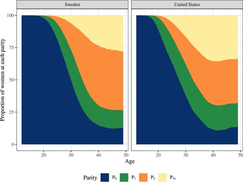
Taking Sweden and the US as an example, Figure 1 provides a graphic representation of the survivorship vector, that is, $\underset{\_}{l^c}(x,t-x{)}^{\mathrm{\prime }}$ in equation (1). Each age corresponds to the parity-specific distribution for the cohort reaching that age in 2015. For example, among the Swedish female cohort born in 1985 and reaching age 30 in 2015, 50 per cent of women were childless at the time of the study, 23 per cent had one child, and 27 per cent had two or more children, whereas in the US, these proportions were 38, 24, and 38 per cent, respectively. Among women born in 1966 and reaching age 49 in 2015 (the oldest cohort contributing to CALP in 2015) in Sweden and the US, respectively, 13 and 14 per cent were childless, 13 and 18 per cent had one child, 35 and 17 per cent had two children, and 38 and 51 per cent had three or more children by then. In Figure 1, the darkest shaded area of parity zero corresponds to the average number of years women of reproductive age could expect to spend childless, as quantified by $\mathrm{C}\mathrm{A}\mathrm{L}{\mathrm{P}}_0\left(2015\right)$. Similarly, the second darkest shaded area of parity one corresponds to the average number of years women of reproductive age could expect to spend at parity one ($\mathrm{C}\mathrm{A}\mathrm{L}{\mathrm{P}}_1\left(2015\right)$), and so on.

Figure 1 Parity-specific cohort survivors by exact age reached in 2015: women in Sweden and the US

Source: Authors’ calculations based on data from the Human Fertility Database.

Cross-sectional average length of life by parity

Table 2 shows the values of $\mathrm{C}\mathrm{A}\mathrm{L}{\mathrm{P}}_i\left(2015\right)$ in 12 countries. Larger numbers refer to a longer average time (in years) spent at each parity by the female population of reproductive age. Ranks are assigned to values in descending order according to time at parity zero—$\mathrm{C}\mathrm{A}\mathrm{L}{\mathrm{P}}_0\left(2015\right)$—and reported in parentheses separately for each parity. We conducted a robustness check to analyse parity from parity zero to parities five and higher (instead of three and higher), and the results were similar to the main ones shown in this paper (detailed results can be found in the supplementary material, Appendix D). In all countries, women stayed childless (i.e. at parity zero) for the largest share of their reproductive years. Among the countries studied, this share was highest in Japan (61 per cent) and Spain (59 per cent) and lowest in the US (46 per cent) and Belarus (42 per cent). The cross-national averages for the time spent at each parity were 19.7 years (at parity zero), 6.6 (at parity one), 8.2 (at parity two), and 3.6 (at parities three and higher). Overall, in countries where women spent comparatively longer at parity zero ($\mathrm{C}\mathrm{A}\mathrm{L}{\mathrm{P}}_0\left(2015\right)$), women were more likely to spend fewer years at parities one ($\mathrm{C}\mathrm{A}\mathrm{L}{\mathrm{P}}_1\left(2015\right)$) and two ($\mathrm{C}\mathrm{A}\mathrm{L}{\mathrm{P}}_2\left(2015\right)$). This finding has a clear explanation in that countries where women had already remained childless for large proportions of their reproductive lives had fewer years left to enter higher parities and, therefore, to stay at these parities. This relationship is also affected by the share of women staying childless throughout their lives because such women contribute no years at higher parities. Further, a short time spent at parity one may also result from transitions to parity two that occur relatively quickly and/or more transitions to parity two, whereas a longer time at parity one indicates that transitions to the next parity are slower and/or fewer transitions happen. For example, Japan and Spain were characterized by similar and relatively large amounts of time spent childless in the female population, but Japanese women showed a lower duration at parity one compared with Spanish women. This difference could indicate the former’s higher propensity to transition to parity two and/or a faster speed in doing so. Next, we categorize countries according to their CALP values.

Table 2 Values of CALP in 2015 in 12 countries and country ranking by parity

	$P_0$		$P_1$		$P_2$		$P_{3+}$
Japan	23.24	(1)	4.97	(10)	6.93	(12)	2.86	(9)
Spain	22.50	(2)	6.89	(5)	6.98	(11)	1.62	(12)
Canada	21.07	(3)	5.16	(9)	7.61	(8)	4.16	(4)
Hungary	20.37	(4)	6.76	(6)	7.09	(10)	3.78	(6)
Denmark	20.02	(5)	4.77	(12)	8.85	(5)	4.36	(2)
Poland	19.99	(6)	6.93	(4)	7.72	(7)	3.37	(7)
Sweden	19.84	(7)	4.79	(11)	9.02	(4)	4.35	(3)
Czechia	19.15	(8)	6.35	(7)	9.66	(1)	2.84	(10)
Lithuania	18.12	(9)	7.73	(3)	9.17	(3)	2.98	(8)
Estonia	18.01	(10)	7.85	(2)	8.29	(6)	3.85	(5)
United States	17.48	(11)	6.17	(8)	7.46	(9)	6.90	(1)
Belarus	15.98	(12)	10.44	(1)	9.22	(2)	2.36	(11)
Average	19.65		6.57		8.17		3.62

Note: The lowest rank (1) indicates the longest amount of time (in years) spent at a parity. Countries are ordered by rank of $P_0$.

Source: Authors’ calculations based on data from the Human Fertility Database.

Countries with lowest-low fertility: Japan and Spain

Women in Japan spent the largest share of their reproductive life childless, corresponding to nearly two-thirds of their entire reproductive life (23.2 years). Japan was closely followed by Spain in this respect (22.5 years). Moving to time at parity one, Japanese women spent less time at parity one (5.0 years) than Spanish women (6.9 years), and their $\mathrm{C}\mathrm{A}\mathrm{L}{\mathrm{P}}_1\left(2015\right)$ value was one of the lowest among the countries we analysed. This finding should be viewed in light of Japanese women’s very late entry into motherhood and the country’s large share of women remaining childless (Frejka et al. 2010), factors which also imply relatively few years spent at risk of reaching higher parities. In addition to women experiencing fewer years at risk of a second child, relatively high rates of transition to parity two may explain this finding (Zeman et al. 2018). On the other hand, in Spain, a prolonged time spent childless was accompanied by a relatively large amount of time at parity one. Hence, mothers of one child in Spain may be more likely to delay or forego a second child compared with their counterparts in Japan and some other countries.

Eastern European countries: Belarus, Estonia, and Lithuania

The common feature of the Eastern European countries studied was that, on average, women spent relatively few years childless and many years at parities one and two. The estimated years of childless life corresponded to approximately 18 years in Estonia and Lithuania and a low of 16 years in Belarus. In turn, women in these three countries could expect to spend the largest amounts of time at parity one compared with women in other countries. In particular, women in Belarus showed the lowest duration at parity zero but the highest duration at parity one (and, similarly, the second highest at parity two) out of the countries analysed. These findings are likely to reflect the well-known pattern where low fertility in these countries results from a decline in completed family size despite relatively early and universal entry into motherhood (Lesthaeghe and Moors 2000; Stankuniene and Jasilioniene 2008).

Central European countries: Czechia, Hungary, and Poland

Central European countries can be found in the middle of the list for expected time spent both childless (around 20 years) and at parity one (approximately six or seven years). In this group of countries, the postponement of childbearing has been relatively modest, whereas the proportion remaining childless has increased although still remaining at a relatively low level among cohorts born in the 1960s and early 1970s (Mynarska 2010; Sobotka 2017). The generally slow transition to first birth was not compensated by a faster transition to second birth in Hungary or Poland, indicating that women in these countries could expect to spend the majority of their reproductive years childless or as a mother of an only child, on average. In Czechia, however, women spent much more time at parity two than at parity one, and the time spent at parity two in Czechia was actually the longest among all the analysed countries. This possibly relates to the strong two-child norm in Czechia (Zeman 2018).

North America: Canada and the US

Canada and the US showed differing trends for parity zero: women in Canada spent a longer average time childless than their counterparts in the US. In turn, the patterns of time spent at parities one and two were similar in the two countries. In terms of spending time at parities three and higher, these two countries were among the top ranked. The US stood out particularly here: women in the US (6.9 years) spent 2.7 years more at parities three and higher on average than their counterparts in Canada (4.2 years). Unlike for Canada, the findings for the US are most likely influenced by its relatively high teenage fertility (Sedgh et al. 2015), lowering the average years spent childless and leaving time for higher parity transitions, which remain relatively common (Santelli and Melnikas 2010; Manning and Cohen 2015; Zeman et al. 2018). Additionally, minority groups in the US (particularly the Hispanic ethno-racial group) have maintained higher fertility compared with minority groups in Canada, which partially explains the longer expected time spent by US women at parities three and higher compared with their Canadian counterparts (Belanger and Ouellet 2002).

The Nordic experience

In Denmark and Sweden, women could expect to stay childless for approximately 20 years of their reproductive life and then to remain at parity one for under five years. The expected time childless sits in the middle of the range of the countries analysed and is followed by the shortest time at parity one. The time spent at higher parities sits in the higher rankings across countries. These findings fit well with prior evidence showing that, despite the trend towards delaying first births, the comprehensive family policies in these countries have led to a strong recuperation of births at older reproductive ages (Andersson et al. 2009). The shares of women remaining ultimately childless in Denmark and Sweden have remained low to average (Sobotka 2017; Jalovaara et al. 2019), and the shares of women having at least two children have remained more stable than in many other high-income countries (Frejka and Sardon 2006; Zeman et al. 2018).

Age and cohort decomposition of CALP: Sweden vs the US

The decomposition by age and cohort of the differences between two CALPs is now illustrated by comparing Sweden and the US, two countries distinct in their CALPs and in the societal context of childbearing. Public policy for families in the US is weak compared with that of Sweden, and gender equality is also not as high (Tsuya et al. 2000; Esping-Andersen 2009). Ethnic and religious diversity contributes to stronger variation in fertility behaviour within the US, and its rates of early childbearing are comparatively high among non-white women (Sutton and Mathews 2004; Lesthaeghe and Neidert 2006). The difference in the time spent childless between the US (17.48) and Sweden (19.84), calculated as $\mathrm{C}\mathrm{A}\mathrm{L}{\mathrm{P}}_0\left(\mathrm{U}\mathrm{S}\right)-\mathrm{C}\mathrm{A}\mathrm{L}{\mathrm{P}}_0\left(\mathrm{S}\mathrm{w}\mathrm{e}\mathrm{d}\mathrm{e}\mathrm{n}\right)=-2.36$ years, is decomposed to reveal age- and cohort-specific contributions (see Figure 2). Similarly, Figures 3 and 4 present the decomposition of the differences in $\mathrm{C}\mathrm{A}\mathrm{L}{\mathrm{P}}_1\left(2015\right)$ and $\mathrm{C}\mathrm{A}\mathrm{L}{\mathrm{P}}_2\left(2015\right)$ for the same two countries.

Figure 2 Lexis surface for the age- and cohort-specific contributions to the difference in $\mathrm{C}\mathrm{A}\mathrm{L}{\mathrm{P}}_0\left(2015\right)$ between the US (17.48) and Sweden (19.84): women born 1966–2003

Note: Positive values (darker tones) correspond to a lower decrease in population at parity zero in the US than Sweden. In contrast, negative values (lighter tones) represent a greater decrease in the US than Sweden.

Source: As for Figure 1.

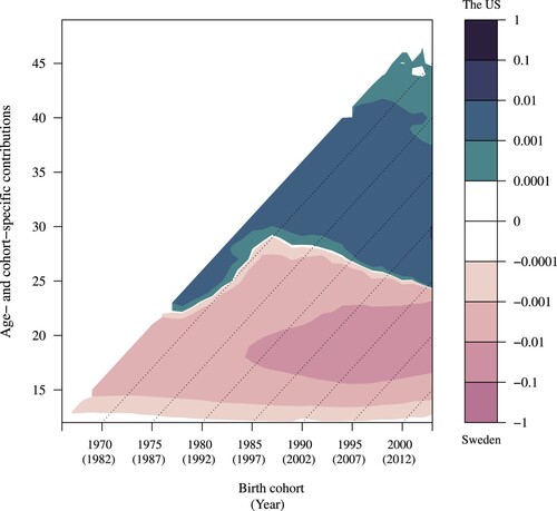
Figure 3 Lexis surface for age- and cohort-specific contributions to the difference in $\mathrm{C}\mathrm{A}\mathrm{L}{\mathrm{P}}_1\left(2015\right)$ between the US (6.17) and Sweden (4.79): women born 1966–2003

Note: Positive values (lighter tones) correspond to a greater relative change in population at parity one in the US than Sweden. In contrast, negative values (darker tones) represent a lower relative change in the US than Sweden.Source: As for Figure 1.

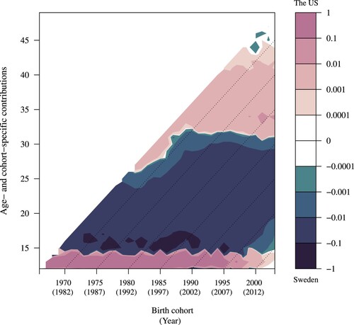
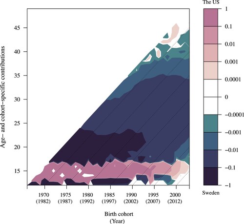
Figure 4 Lexis surface for age- and cohort-specific contributions to the difference in $\mathrm{C}\mathrm{A}\mathrm{L}{\mathrm{P}}_2\left(2015\right)$ between the US (7.46) and Sweden (9.02): women born 1966–2003

Note: Positive values (lighter tones) correspond to a greater relative change in population at parity two in the US than Sweden. In contrast, negative values (darker tones) represent a lower relative change in the US than Sweden.Source: As for Figure 1.

In Figure 2, positive values (darker tones) refer to smaller decreases with age in the female population at parity zero in the US than in Sweden, whereas negative values (lighter tones) refer to the opposite (greater decreases with age in the US); note that the population at parity zero can only decrease and not increase with age. For some ages and cohorts, the contributions to the difference between $\mathrm{C}\mathrm{A}\mathrm{L}{\mathrm{P}}_0\left(\mathrm{U}\mathrm{S}\right)$ and $\mathrm{C}\mathrm{A}\mathrm{L}{\mathrm{P}}_0\left(\mathrm{S}\mathrm{w}\mathrm{e}\mathrm{d}\mathrm{e}\mathrm{n}\right)$ were zero (indicated by the white colour), corresponding to equal decreases in childlessness with age in Sweden and the US. In Figure 2, there is a clear colour switch between the ages of 20 and 30, separated by a broadly horizontal white line. This change indicates that at young ages (below the white line), a greater decrease with age in the female population at parity zero (i.e. more women becoming mothers) in the US relative to Sweden contributed to the higher $\mathrm{C}\mathrm{A}\mathrm{L}{\mathrm{P}}_0$ in Sweden than in the US. In other words, Swedish women were more likely to remain childless in the first decade of their reproductive life compared with US women. By contrast, the higher transition rates to first births among older Swedish women relative to US women (above the white line) made a negative contribution to $\mathrm{C}\mathrm{A}\mathrm{L}{\mathrm{P}}_0$ in Sweden relative to the US.

The pattern at ages below 30 can be explained by high teenage fertility in the US, where teenage fertility is still at a level among the highest in the developed world (Boonstra 2002) and substantially higher than in Sweden (McKay and Barrett 2010). At older reproductive ages (30 and above) the situation is reversed, with higher transitions to parity one in Sweden than in the US. This difference, in turn, is likely to reflect the fertility postponement and strong recuperation of births at older ages typical of the Nordic fertility regime (Andersson et al. 2009). We also note that the threshold age for switching from negative to positive values sharply increases around the late 1960s cohorts and then decreases from the cohorts born in 1970, indicating that the Swedish women’s catching-up behaviour compared with that of the US women becomes less apparent in the younger cohorts. Furthermore, differences in the change in the young population at parity zero between Sweden and the US are most prominent between 1997 and 2015, which partly reflects an increase in the teenage pregnancy rate in the US in the late 1980s (Kearney and Levine 2012).

The 1.38-year difference in $\mathrm{C}\mathrm{A}\mathrm{L}{\mathrm{P}}_1$ between the US (6.17) and Sweden (4.79) is presented in Figure 3. As explained in the previous section and supplementary material (Appendix C) as well as in Table 1, the interpretation of the country comparison ratio becomes opposite for parity zero than for parities one and higher. Therefore, in Figures 3 and 4, positive values (lighter tones) correspond to a greater relative change in population at parities one and higher in the US than in Sweden. In contrast, negative values (darker tones) represent a lower relative change in the US than Sweden. In Figure 3, there is also a colour switch, as seen in Figure 2, separated by a broadly horizontal white line at around age 30 for the cohorts born after 1970 (or at a younger age for the cohorts born before 1970). The negative values indicate lower growth in the population of women at parity one by age in the US relative to Sweden. In other words, below the broadly horizontal line, and following the early transition to first birth observed in Figure 2, it can be assumed that women in the US were also more likely to transition to second births at early ages than women in Sweden.

When summed over cohorts, these changes led to a higher $\mathrm{C}\mathrm{A}\mathrm{L}{\mathrm{P}}_1\left(2015\right)$ in the US than Sweden, meaning that, on average, women in the US spent more time at parity one than women in Sweden. The total contribution to the difference in $\mathrm{C}\mathrm{A}\mathrm{L}{\mathrm{P}}_1$ between Sweden and the US was largest at ages under 15 where the contribution was positive (20.1); in contrast there was a negative contribution for middle reproductive ages (−19.5) and a small positive contribution at older ages (0.7). Therefore, the larger growth at ages under 15 in the US widened the difference in $\mathrm{C}\mathrm{A}\mathrm{L}{\mathrm{P}}_1$, but the greater growth in Sweden at the middle ages narrowed the gap. Finally, the greater growth in the US at the later ages did not contribute much.

Moving to Figure 4, the decomposition of the −1.56-year difference in $\mathrm{C}\mathrm{A}\mathrm{L}{\mathrm{P}}_2$ between the US (7.46) and Sweden (9.02) shows partially similar trends to Figure 3 for parity one. The higher fertility of adolescents in the US, more likely to have a second birth in their teens compared with adolescents in Sweden, represents the only positive relative change (growth) in the population at parity two for the US. At older ages and for all cohorts, the opposite trend can be observed, with higher growth in the population at parity two for Swedish women at all ages, except for the teenage years. This trend reflects the strong two-child norm in Sweden (Oláh and Bernhardt 2008; Kirmeyer and Hamilton 2011), meaning that for the majority of women, the transition to parity two represents the completion of family formation. Transitions to parity two seem to be more concentrated at higher reproductive ages in Sweden than in the US. As observed in Table 2, US women also spent the longest time at parities three and higher relative to women in the other countries analysed. This finding may reflect either the higher age-specific transition rates to higher parities in the US or the influence of earlier overall fertility timing in the US, leaving more time at the highest parities than in Sweden. Prior evidence indicates that both explanations are likely to be relevant (Frejka and Sardon 2006; Zeman et al. 2018).

Discussion

The fertility indicator introduced by this study—cross-sectional average length of life by parity (CALP)—is an alternative way of summarizing the cohort fertility behaviour of a population in a period perspective by considering the dynamics of parity transitions. CALP measures the average duration (in years) spent at each parity by women between 12 and 50 years of age. Unlike conventional period fertility measures, CALP uses all available cohort information on the parity-specific birth histories of women of reproductive age at a given point in time. This study added substantial value by presenting comparisons of CALP for 12 countries and by quantifying the age- and cohort-specific contributions to the differences in CALPs between two example countries.

Our results for 2015 showed that in those countries where women spend comparatively longer time on average at parity zero, they also spend fewer years at parities one and two. We categorized the countries studied into five groups based on their CALP values. In countries with lowest-low fertility (Japan and Spain), women can expect to spend the largest share of their reproductive life childless compared with women in other countries. In the Eastern European countries (Belarus, Estonia, and Lithuania), women spend a relatively short average length of time childless but can expect to spend relatively more years at parities one and two. The Central European countries (Czechia, Hungary, and Poland) are in the middle of the list in terms of both expected years spent childless and at parity one. In the Northern European countries (Denmark and Sweden), the expected time childless sits in the middle of the range of the countries analysed and is then followed by the shortest time spent at parity one. Finally, North American countries (Canada and the US) are characterized as being among the top ranked in terms of years women spend at parities three and higher.

Further, the differences between the CALPs for Sweden and the US in 2015 were decomposed into age- and cohort-specific contributions, as an illustrative case considering the marked differences in their societal contexts of childbearing, for example in fertility timing, ethnic and religious diversity, norms, and public policies (Tsuya et al. 2000; Sutton and Mathews 2004; Lesthaeghe and Neidert 2006; Oláh and Bernhardt 2008; Esping-Andersen 2009; Kirmeyer and Hamilton 2011). The decomposition results should be interpreted as the relative change in a country’s female population at a given parity i at each specific age and cohort, relative to its initial counts of women at the same parity. The comparison of decomposition results for Sweden and the US highlighted how high teenage fertility in the US dominates the differences between the two countries in the time spent at different parities.

There is a strong link between childbearing timing and quantum. For example, higher age at entering parity one leaves less time for any higher parity transitions to be realized (Beaujouan et al. 2019). This can be due to a number of factors, including the direct age-related decline in fecundity (ESHRE Capri Workshop Group 2005), the existence of social age deadlines for childbearing (Settersten and Hagestad 1996; Billari et al. 2011), the development of interests in alternative lifestyles that are not compatible with childbearing (Carmichael and Whittaker 2007), and the revision of fertility desires downwards when it is perceived that they are un-likely to be fulfilled (Gray et al. 2013). A large share of those women who have their first child at a later age might also express an early preference for fewer children (Rindfuss et al. 1980), although it is unlikely that many women overall hold childlessness preferences from an early age (Toulemon 1996). Despite their advantages in terms of straightforward interpretation, the common indicators used for measuring either fertility timing or fertility quantum may, in fact, be partially limited in the way that they do not capture this relationship. CALP is an attempt to connect both timing and quantum of fertility by combining these dimensions into an informative series of $\mathrm{C}\mathrm{A}\mathrm{L}{\mathrm{P}}_i$ measures. Therefore, the value of $\mathrm{C}\mathrm{A}\mathrm{L}{\mathrm{P}}_i$ depends on: (1) how many women progress to the next parity (quantum); and (2) when such progression is made (timing).

Limitations of this study should be acknowledged. First, as a macro-level measure, CALP is the outcome of several population-level processes and, therefore, its contribution in revealing fertility behaviour is limited (i.e. its interpretation in terms of fertility behaviour may benefit from integrating other sources of information as we have done in this paper). However, we note that other aggregate demographic measures, such as the TFR and MAC, are extensively used in fertility research, despite having similar limitations; hence, this limitation should not detract researchers from using CALP. Second, the calculation of CALP requires a long time series of birth data by age and parity and, thus, its use is restricted to countries that can provide the necessary information. However, CALP could also be calculated as a truncated measure using incomplete cohort birth information, similar to the truncated cross-sectional average length of life (TCAL) developed and used in mortality research (Canudas-Romo and Guillot 2015). Therefore, the truncated version of CALP has more potential to be used in middle- or low-income countries, where a long history of detailed fertility data is less often available.

In summary, CALP provides an alternative perspective for studying population-level fertility patterns, given its three methodological advantages: (1) being a period fertility indicator using all available cohort information; (2) capturing the dynamics of parity transitions; and (3) linking information on fertility quantum and timing together as part of a single phenomenon. In addition, the decomposition of CALPs can show which of two countries is experiencing a greater/smaller growth or decrease (relative change) in its female population at a given parity, and for each specific age and cohort. There are also some other reasons for applying this measure. Because analysing population growth is fundamental in demographic research, we believe that CALP adds to the previously used similar fertility measures in terms of substance, and that its interpretation is relatively intuitive for demographers. From a broader perspective, CALP may provide relevant information, for instance for policymakers in the area of employment in contexts where women’s employment strongly depends on their number of children. Finally, we believe that the time spent at each parity is a relevant aspect of the reproductive life experience of a female population and therefore worth the attention of demographers. For all these reasons, CALP provides another useful demographic analytic tool for studying aggregate fertility patterns across countries and over time. The results of this study showed that countries differ in systematic ways with regard to the time that women spend on average at different parities during their reproductive lives.

Disclosure statement

No potential conflict of interest was reported by the authors.

Notes

1 Please direct all correspondence to Ryohei Mogi, 42–43 Park End Street, Oxford, OX1 1JD, UK; or by Email: [email protected]

2 Ryohei Mogi is based in the Department of Sociology, the Leverhulme Centre for Demographic Science, and Nuffield College at the University of Oxford. Ester Lazzari and Vladimir Canudas-Romo are based in the School of Demography, The Australian National University. Jessica Nisén is based at the INVEST Research Flagship, University of Turku, Finland, and also the Max Planck Institute for Demographic Research.

3 This research has received funding from the European Research Council under the European Union’s Horizon 2020 research and innovation programme under grant agreement no. 681546 (FAMSIZEMATTERS). Ester Lazzari was supported by the University Research Scholarship and by the Higher Degree Research Fee Merit Scholarship offered by the Australian National University. Jessica Nisén was supported by the Academy of Finland (no. 332863 and no. 320162) and the Strategic Research Council (FLUX, no. 345130).

4 We are grateful to the Population Studies copyeditor for their careful editing and revisions to polish the manuscript.

References

- Andersson, G., M. Rønsen, L. B. Knudsen, T. Lappegård, G. Neyer, K. Skrede, K. Teschner, and A. Vikat. 2009. Cohort fertility patterns in the Nordic Countries, Demographic Research 20(14): 313–352. https://doi.org/10.4054/DemRes.2009.20.14
- Beaujouan, E., A. Reimondos, E. Gray, A. Evans, and T. Sobotka. 2019. Declining realisation of reproductive intentions with age, Human Reproduction 34(10): 1906–1914. https://doi.org/10.1093/humrep/dez150
- Belanger, A. and G. Ouellet. 2002. A comparative study of recent trends in Canadian and American fertility, 1980–1999, in Statistics Canada (ed), Report on the Demographic Situation in Canada 2001. Ottawa: Statistics Canada, pp. 107–136.
- Billari, F. C., A. Goisis, A. C. Liefbroer, R. A. Settersten, A. Aassve, G. Hagestad, and Z. Spéder. 2011. Social age deadlines for the childbearing of women and men, Human Reproduction 26(3): 616–622. https://doi.org/10.1093/humrep/deq360
- Bongaarts, J. and G. Feeney. 1998. On the quantum and tempo of fertility, Population and Development Review 24(2): 271–291. https://doi.org/10.2307/2807974
- Bongaarts, J. and T. Sobotka. 2012. A demographic explanation for the recent rise in European fertility, Population and Development Review 38(1): 83–120. https://doi.org/10.1111/j.1728-4457.2012.00473.x
- Boonstra, H. D. 2002. Teen pregnancy: Trends and lessons learned, The Guttmacher Report on Public Policy 5(1): 1–4.
- Brouard, N. 1986. Structure et dynamique des populations. La pyramide des années à vivre, aspects nationaux et exemples régionaux (Structure and dynamics of populations. The later-life pyramid, national aspects and regional examples), Espace, Populations, Sociétés 2(14–15): 157–168. https://doi.org/10.3406/espos.1986.1120
- Canudas-Romo, V. and M. Guillot. 2015. Truncated cross-sectional average length of life: A measure for comparing the mortality history of cohorts, Population Studies 69(2): 147–159. https://doi.org/10.1080/00324728.2015.1019955
- Carmichael, G. and A. Whittaker. 2007. Choice and circumstance: Qualitative insights into contemporary childlessness in Australia, European Journal of Population 23(2): 111–143. https://doi.org/10.1007/s10680-006-9112-4
- ESHRE Capri Workshop Group. 2005. Fertility and ageing, Human Reproduction Update 11(3): 261–276. https://doi.org/10.1093/humupd/dmi006
- Esping-Andersen, G. 2009. Incomplete Revolution: Adapting Welfare States to Women’s New Roles. Cambridge: Polity.
- Frejka, T., G. W. Jones, and J.-P. Sardon. 2010. East Asian childbearing patterns and policy developments, Population and Development Review 36(3): 579–606. https://doi.org/10.1111/j.1728-4457.2010.00347.x
- Frejka, T. and J.-P. Sardon. 2006. First birth trends in developed countries: Persisting parenthood postponement, Demographic Research 15(6): 147–180. https://doi.org/10.4054/DemRes.2006.15.6
- Frejka, T. and T. Sobotka. 2008. Overview chapter 1: Fertility in Europe: Diverse, delayed and below replacement, Demographic Research 19(3): 15–46. https://doi.org/10.4054/DemRes.2008.19.3
- Gray, E., A. Evans, and A. Reimondos. 2013. Childbearing desires of childless men and women: When are goals adjusted?, Advances in Life Course Research 18(2): 141–149. https://doi.org/10.1016/j.alcr.2012.09.003
- Guillot, M. 2003. The cross-sectional average length of life (CAL): A cross-sectional mortality measure that reflects the experience of cohorts, Population Studies 57(1): 41–54. https://doi.org/10.1080/0032472032000061712
- Human Fertility Database (HFD) organized by Max Planck Institute for Demographic Research (Germany) and Vienna Institute of Demography (Austria). HFD is available at www.humanfertility.org (data downloaded on August 2018).
- Jalovaara, M., G. Neyer, G. Andersson, J. Dahlberg, L. Dommermuth, P. Fallesen, and T. Lappegård. 2019. Education, gender, and cohort fertility in the Nordic countries, European Journal of Population 35: 563–586. https://doi.org/10.1007/s10680-018-9492-2
- Kearney, M. S. and P. B. Levine. 2012. Why is the teen birth rate in the United States so high and why does it matter?, Journal of Economic Perspectives 26(2): 141–166. https://doi.org/10.1257/jep.26.2.141
- Kirmeyer, S. E. and B. E. Hamilton. 2011. Childbearing Differences among Three Generations of U.S. Women. NCHS data brief, no. 68. Hyattsville, MD: National Center for Health Statistics.
- Kohler, H.-P. and J. A. Ortega. 2002. Tempo-adjusted period parity progression measures, fertility postponement and completed cohort fertility, Demographic Research 6(6): 91–144. https://doi.org/10.4054/DemRes.2002.6.6
- Lesthaeghe, R. J. and G. B. D. Moors. 2000. Recent trends in fertility and household formation in the industrialized world, Review of Population and Social Policy 9: 121–170.
- Lesthaeghe, R. J. and L. Neidert. 2006. The second demographic transition in the United States: Exception or textbook example?, Population and Development Review 32(4): 669–698. https://doi.org/10.1111/j.1728-4457.2006.00146.x
- Luy, M. 2011. Tempo effects and their relevance in demographic analysis, Comparative Population Studies 35(3): 415–446. https://doi.org/10.12765/CPoS-2010-11
- Manning, W. D. and J. A. Cohen. 2015. Teenage cohabitation, marriage, and childbearing, Population Research and Policy Review 34(2): 161–177. https://doi.org/10.1007/s11113-014-9341-x
- McKay, A. and M. Barrett. 2010. Trends in teen pregnancy rates from 1996–2006: A comparison of Canada, Sweden, U.S.A., and England/Wales, The Canadian Journal of Human Sexuality 19(1-2): 43–52.
- Morgan, S. P. and R. R. Rindfuss. 1999. Reexamining the link of early childbearing to marriage and to subsequent fertillty, Demography 36: 59–75. https://doi.org/10.2307/2648134
- Mogi, R. and V. Canudas-Romo. 2020. Cross-sectional average length of life by parity: Illustration for the US cohorts in reproductive ages in 2015, in R. Schoen (ed), Analyzing Contemporary Fertility. Berlin/Heidelberg, Germany: Springer, pp. 293–306. https://doi.org/10.1007/978-3-030-48519-1_13
- Mogi, R., J. Nisén, and V. Canudas-Romo. 2021. Cross-sectional average length of life childless, Demography 58(1): 321–344. https://doi.org/10.1215/00703370-8937427
- Mynarska, M. 2010. Deadline for parenthood: Fertility postponement and age norms in Poland, European Journal of Population 26: 351–373. https://doi.org/10.1007/s10680-009-9194-x
- Oláh, L. S. and E. M. Bernhardt. 2008. Sweden: Combining childbearing and gender equality, Demographic Research 19(28): 1105–1144. https://doi.org/10.4054/DemRes.2008.19.28
- Preston, S., P. Heuveline, and M. Guillot. 2001. Demography: Measuring and Modelling Population Processes. Oxford: Blackwell.
- Rindfuss, R. R., L. Bumpass, and C. St. John. 1980. Education and fertility: Implications for the roles women occupy, American Sociological Review 45(3): 431–447. https://doi.org/10.2307/2095176
- Ryder, N. B. 1964. The process of demographic translation, Demography 1(1): 74–82. https://doi.org/10.1007/BF03208446
- Santelli, J. S. and A. J. Melnikas. 2010. Teen fertility in transition: Recent and historic trends in the United States, Annual Review of Public Health 31: 371–383. https://doi.org/10.1146/annurev.publhealth.29.020907.090830
- Schmidt, L., T. Sobotka, J. G. Bentzen, A. Nyboe Andersen, and ESHRE Reproduction and Society Task Force. 2012. Demographic and medical consequences of the postponement of parenthood, Human Reproduction Update 18(1): 29–43. https://doi.org/10.1093/humupd/dmr040
- Schoen, R. 2004. Timing effects and the interpretation of period fertility, Demography 41: 801–819. https://doi.org/10.1353/dem.2004.0036
- Schoen, R. 2016. Hierarchical multistate models from population data: An application to parity statuses, PeerJ 4(e2535): 1–11. https://doi.org/10.7717/peerj.2535
- Schoen, R. 2020. Measuring the prevalence of multipartner fertility independent of fertility level, in R. Schoen (ed), Analyzing Contemporary Fertility. Springer, pp. 287–292. https://doi.org/10.1007/978-3-030-48519-1_12
- Sedgh, G., L. B. Finer, A. Bankole, M. A. Eilers, and S. Singh. 2015. Adolescent pregnancy, birth, and abortion rates across countries: Levels and recent trends, Journal of Adolescent Health 56(2): 223–230. https://doi.org/10.1016/j.jadohealth.2014.09.007
- Settersten, R. A. and G. O. Hagestad. 1996. What’s the latest? Cultural age deadlines for family transitions, The Gerontologist 36: 602–613. https://doi.org/10.1093/geront/36.5.602
- Sobotka, T. 2017. Childlessness in Europe: Reconstructing long-term trends among women born in 1900–1972, in M. Kreyenfeld and D. Konietzka (eds), Childlessness in Europe: Contexts, Causes, and Consequences. Cham: Springer International Publishing, pp. 17–53.
- Stankuniene, V. and A. Jasilioniene. 2008. Lithuania: Fertility decline and its determinants, Demographic Research 19(20): 705–742. https://doi.org/10.4054/DemRes.2008.19.20
- Sutton, P. D. and T. Mathews. 2004. Trends in characteristics of births by state: United States, 1990, 1995, and 2000–2002, National Vital Statistics Reports 52(19): 1–18.
- Tomkinson, J. 2019. Age at first birth and subsequent fertility: The case of adolescent mothers in France and England and Wales, Demographic Research 40(27): 761–798. https://doi.org/10.4054/DemRes.2019.40.27
- Toulemon, L. 1996. Very few couples remain voluntarily childless, Population: an English Selection 8: 1–27.
- Tsuya, N. O., L. L. Bumpass, and M. K. Choe. 2000. Gender, employment, and housework in Japan, South Korea, and the United States, Review of Population and Social Policy 9(9): 195–220.
- Zeman, K. 2018. Cohort fertility and educational expansion in the Czech Republic during the 20th century, Demographic Research 38(56): 1699–1732. https://doi.org/10.4054/DemRes.2018.38.56
- Zeman, K., É. Beaujouan, Z. Brzozowska, and T. Sobotka. 2018. Cohort fertility decline in low fertility countries: Decomposition using parity progression ratios, Demographic Research 38(25): 651–690. https://doi.org/10.4054/DemRes.2018.38.25