Estimating age-specific mortality using calibrated splines

Abstract

Demographers have developed a number of methods for expanding abridged mortality data into a complete schedule; however, these can be usefully applied only under certain conditions, and the presence or absence of one or more additional sources of incompleteness can degrade their relative accuracy, lead to implausible profiles, or even cause the methods to fail. We develop a new method for expanding an abridged schedule based on calibrated splines; this method is accurate and robust in the presence of errors in mortality rates, missing values, and truncation. We compare its performance with the performance of existing methods for expanding abridged data and find that it is superior to current methods at producing accurate and plausible complete schedules over a broad range of data-quality conditions. The method when applied is a valuable addition to existing tools for estimating mortality, especially for small nations, countries with incomplete vital statistics, and subnational populations.

Keywords:

• abridged life table
• mortality rates
• calibrated splines
• methods

Introduction

The life table is one of demography’s most enduring contributions to science. From its introduction by Graunt (1662) to study survival fractions in London, its use has spread within demography to studies of fertility (Arunachalam 2004), migration (Rogers 1975), population projections (UN 1968), and beyond, to insurance and capital markets (Halley 1693; Dickson et al. 2019; Blake and Cairns 2021), epidemiology (Greville 1948), and government finance and policymaking (e.g. Treasury 2015; NIAA 2020). Indeed, the life expectancy column in the table is now widely accepted as a measure of societal equity, a way to describe gaps in equity among subpopulations, and a driver for policy to address such gaps (CSDH 2008; Taylor and Barnes 2013).

The twentieth century saw significant reductions in global and national mortality rates through advances in global wealth, medicine, and science (Riley 2005a; UN 2022). However, while life expectancy is estimated to have increased globally from 28.5 years in 1800 to 71.0 years in 2021, there is recognition that this increase has not been linear over time (or even monotonic), with inequalities persisting both between and within countries (Riley 2005b; UN 2012, 2022). Understanding the characteristics and causes of international and subnational mortality heterogeneity therefore remains a focus for demographers, public health administrators, and governments at all levels. This is in part because of the compelling nature of the life expectancy statistic as a composite diagnostic for the overall health, equality, and governance of societies and their subpopulations and also as a comparator, ceteris paribus, between subpopulations and nations (Marmot 2015).

The basis for the construction of a life table is a complete schedule of death rates: the ratio of the number of deaths to the population exposed to the risk of dying. In this context, ‘complete’ means an accurate set referencing a contiguous sequence of one-year age intervals, beginning at age 0 and terminating at an age $\omega$ (e.g. 110 years) beyond which survival is either rare or rates may be assumed to be constant. Given a complete schedule, standard methods can be applied to convert rates into probabilities, survival fractions, person-years lived, and life expectancies (Chiang 1984; Wilmoth et al. 2007). The complete life table is also used to calculate summary measures of the death distribution that go beyond its first moment (life expectancy), including outsurvival (Vaupel et al. 2021), and compression and delay (Fries 1980; Vaupel 2010; de Beer and Janssen 2016). Often, however, mortality data are not complete, with one or more of the conditions of accuracy, contiguity, single-year age intervals, or $\omega$ being high enough not satisfied.

A common form of incompleteness is abridgement, where one or more age intervals are wider than one year. One form of abridgement is the use of an open interval terminating the set of death rates, with the final rate covering an age group of the form ‘$a$ and over’. The open interval cannot be discarded when $a$ is not a reasonable choice for $\omega$ (we call this ‘truncation’), a situation that can arise because a once adequate $a$ is no longer so due to improvements in longevity or because higher values of $a$ might either risk the anonymity of small populations or expose the rates to errors related to age misreporting (Preston et al. 1999). Abridgement can also occur at moderate ages as the result of a strategy to mitigate errors in the rates. The source of such errors can be systematic (from age heaping, e.g. Hobbs 2004) or random (due to sample noise e.g. Chiang 1984).

Users of secondary mortality data will frequently encounter abridged schedules for the reasons just given and because abridgement is a useful way to limit the complexity of full schedules, which are sometimes regarded as overly long and dense (Greenwood 1934). In addition, national statistics offices often publish abridged data to ensure their data are non-disclosive or because the data require abridgement since noise has been added as part of a confidentialization procedure (Fraser and Wooton 2005; Abowd et al. 2019).

To overcome the effects of abridgement on constructing a life table, demographers have developed a number of methods for expanding abridged mortality data into a complete schedule. The regular age pattern of death rates has led to the development of laws of mortality, which take the form of simple parametric functions describing the rapid decline in mortality rates after the first year of life (Oppermann 1870), their rise and fall as young adults mature (Thiele 1871), the exponential increase in mortality as the body ages (Gompertz 1825; Makeham 1860), and the decrease in the mortality slope at advanced years (Thatcher et al. 1998), all of which can be combined to give a description of mortality across the age range (Thiele 1871; Heligman and Pollard 1980; de Beer and Janssen 2016). These parametric models can be used to expand an abridged schedule using non-linear least-squares fitting (UN 1988, 2013; Kostaki 1991).

When errors in the observed rates are small, expansion reduces to interpolation, where one-year rates are inferred subject to the requirements that the multi-year rates are recovered exactly and the complete schedule is smooth. Under these conditions, spline methods can be used to derive a complete schedule from abridged data (Elandt-Johnson and Johnson 1980; Hsieh 1991; Wilmoth et al. 2007). Spline methods have also been extended to handle moderate levels of noise, using P-splines (Rizzi et al. 2015, 2019). Relational methods borrow the age structure of rates from an existing complete schedule (the standard) and apply adjustments to fit abridged rates approximately (Brass 1971) or exactly (Kostaki 2000). The recognition that mortality patterns can be usefully classified into families (UN 1955, 1982, 2011; Coale and Demeny 1966; INDEPTH Network 2002; Li and Gerland 2011) has greatly simplified the problem of the choice of standard.

All these methods can be usefully applied only under certain conditions and, as we shall discuss, the presence or absence of one or more additional sources of incompleteness can degrade their relative accuracy or even cause the methods to fail because they become mathematically undefined. For example, if abridged rates are subject to significant sample noise, then spline methods can produce implausible complete schedules. Likewise, if an abridged rate is zero (because no deaths were recorded in that age interval), it can give negative death probabilities (although death probabilities can also be negative when an abridged rate is positive). Attempting to circumvent these problems by increasing the abridging interval is not necessarily a solution, because spline methods work well when the underlying curve is polynomial between knot points, but when the interval increases this approximation is less valid.

While parametric methods are robust in the presence of noise, they cannot compete with splines for accuracy otherwise. The parameters underlying spline methods, and some in parametric methods, encode local features of the mortality rates which can make these methods unreliable when the data are non-contiguous (because a rate is missing or deemed too unreliable to use). Meanwhile, relational methods readily encode global features (through the standard) but can lack the flexibility of parametric and spline methods due to their relatively low number of fitting parameters (Brass 1971) or may be unstable when data are noisy because they, too, encode local features (Kostaki 2000).

For expanding abridged schedules of fertility rates, the calibrated spline (CS) estimator is a method that integrates the strengths of polynomial, parametric, and relational approaches (Schmertmann 2014). CS combines over-parameterization using B-splines with a structured factoring of shapes using singular value decomposition. It provides the flexibility of a spline method (through over-parameterization), the noise tolerance of a parametric method (because it uses weighted least squares as a fitting metric), and the global properties of a relational method (via a shape penalty term), and it can be solved using the tools of linear algebra. Consequently, the aim of our work is to retain the essence of the CS fertility approach but transform it to the context of mortality, creating a new method for expanding abridged death rates that is accurate and robust in the presence of the other sources of incompleteness already described.

In the next two sections we outline our method for expanding mortality schedules using the CS approach and show how the resulting non-linear equations can be solved using linear regression. Using a test set derived from the Human Mortality Database (HMD), we then compare the accuracy of the CS method to that of spline, relational, and parametric methods under conditions where abridgement and truncation are the dominant sources of incompleteness. We then provide three case studies which illustrate the benefits of our method over and above current domain-specific methods when only imperfect mortality schedules are available to demographers, demonstrating in each case how CS can be applied without modification.

Calibration

We assume that the death rate for the first year of life is known and that the annual death rates for subsequent years up to age $\omega$  =  110 need to be estimated from abridged data. The first step in the CS method is calibration, where for each sex a large representative set of complete mortality curves is reduced to a small set of basis curves using singular value decomposition. To illustrate the process, we constructed a data set spanning a broad historical range and the world’s major regions (UN 2022) and used it to calculate a set of basis curves modelling world human mortality. For the calibration set we chose life tables from the HMD (2016) and World Health Organization (WHO) (WHO 2016).

Within the HMD data set, we used all national populations except Iceland and Luxembourg (which were excluded because their complete mortality rates showed excessive noise, likely a result of sampling variance from their small populations), leaving 35 countries. Even schedules for some large countries showed some amounts of noise. For this reason, we smoothed death rates for the remaining countries using P-splines (Eilers and Marx 1996). From this set of curves, $\mathrm{H}\mathrm{M}{\mathrm{D}}_a$, we chose two disjoint subsets: a calibration set, $\mathrm{H}\mathrm{M}{\mathrm{D}}_c$, containing curves sampled at 10-year intervals beginning with the most recent life table; and a test set, $\mathrm{H}\mathrm{M}{\mathrm{D}}_t$, of curves also sampled at 10-year intervals but shifted by five years relative to the curves in $\mathrm{H}\mathrm{M}{\mathrm{D}}_c$. The result was 332 HMD calibration schedules and 308 HMD test schedules for each sex.

The WHO data set consists of five-year abridged life tables for 192 countries, spanning all subregions of the world (UN 1999) for the year 2000. Using abridged tables is not ideal but is necessary for representing world mortality, because the $\mathrm{H}\mathrm{M}{\mathrm{D}}_a$ data set covers mostly Europe and North America, with little to no data on countries in Africa, Asia, Oceania (apart from Australia and New Zealand), or Latin America and the Caribbean. In particular it contains no countries from two of the world’s fastest growing subregions, sub-Saharan Africa and Central and Southern Asia (UN 2022). Complete schedules of death rates, $\mathrm{W}\mathrm{H}{\mathrm{O}}_c$, were estimated by fitting the nine-parameter Heligman–Pollard model (Heligman and Pollard 1980). Combining $\mathrm{H}\mathrm{M}{\mathrm{D}}_c$ and $\mathrm{W}\mathrm{H}{\mathrm{O}}_c$ gave us for each sex a calibration set containing 524 complete mortality schedules.

For each schedule in a calibration set we constructed the column vector (1) $\mu =\left[\begin{array}{c}{\mu }_1\\ ⋮\\ {\mu }_{\omega }\end{array}\right]$(1) of the force of mortality (2) ${\mu }_x=-\mathrm{l}\mathrm{o}\mathrm{g}\left({\displaystyle \frac{l_{x+1}}{l_x}}\right),x=1,\dots ,\omega ,$(2) where $l_x$ is the survival fraction at age $x$. For each sex these vectors are arrayed columnwise to form an $\omega \times 524$ matrix, $M$. Next, the logarithm of $M$ was factorized using singular value decomposition (Golub and Van Loan 1996) (3) $\mathrm{l}\mathrm{o}\mathrm{g}M=U\cdot S\cdot V^{\mathrm{\prime }},$(3) where $A\cdot B$ denotes matrix multiplication and $A{}^{\mathrm{\prime }}$ is the transpose of $A$. Here and in the following, $A^{-1}$ denotes a matrix inverse, and all other matrix operations and functions act elementwise. The columns of $U$ contain the orthonormal principal components of $\mathrm{l}\mathrm{o}\mathrm{g}M$. We found that in the schedules for both females and males, the first five columns of $U$ accounted for approximately 95 per cent of the variation in $\mathrm{l}\mathrm{o}\mathrm{g}M$.

Figures A1 and A2 in the supplementary material show these five principal components for females and males, respectively. The first component describes the average shape of mortality curves in the calibration set. The remaining components describe the four principal ways in which individual schedules deviate from this average. The second component changes the slope of the entire curve with a pivot point near age 30 for females and age 20 for males. The third component changes the curvature, with ages below 20 and above 50 moving opposite to ages 20–50. Both the fourth and the fifth components change the curvature for ages below 40. Above age 40, the fourth component changes the curvature and the fifth component changes the slope.

Let $X$ be the $\omega \times 5$ matrix of the first five principal components. Given any $\omega \times 1$ force of mortality schedule $\mu$, the $\omega \times \omega$ matrix, (4) $P=X\cdot X^{\mathrm{\prime }},$(4) applied to its logarithm, $\mathrm{l}\mathrm{o}\mathrm{g}\mu$, projects it onto the linear space spanned by the five components. The $\omega \times \omega$ matrix, (5) $\overline{P}=I-P,$(5) applied to the logarithm of the force of mortality schedule will give its shape residual, (6) $e=\overline{P}\cdot \mathrm{l}\mathrm{o}\mathrm{g}\mu ,$(6) the portion of the $\mathrm{l}\mathrm{o}\mathrm{g}\mu$ that cannot be written as a sum of the five components. Although five factors are enough to model 95 per cent of the mortality variation by age for smoothed schedules, observed schedules will contain a component of sample noise that cannot be modelled by these factors and which cause the observed residuals to deviate from zero. For each sex, the scale of the residuals is set by the $\omega \times \omega$ shape covariance matrix, (7) $V_s={\displaystyle \frac{1}{332}\sum _{j\in \mathrm{H}\mathrm{M}{\mathrm{D}}_c}{e}_j\cdot e_j{}^{\mathrm{\prime }},}$(7) where $e_j$ is the shape residual for the $j$th unsmoothed schedule in $\mathrm{H}\mathrm{M}{\mathrm{D}}_c$. The calculation of $V_s$ does not include $\mathrm{W}\mathrm{H}{\mathrm{O}}_c$ curves, because the set does not include unsmoothed, unabridged rates. If $\mathrm{W}\mathrm{H}{\mathrm{O}}_c$ curves were included they would lead to an underestimate of the shape covariance matrix. The calibration stage is only carried out once to calculate, for each sex, a residual matrix, $\overline{P}$, and a shape covariance matrix, $V_s$. Given any abridged curve, the objective of the CS method is now to construct a complete mortality schedule that has a small shape residual and which fits the abridged death rates.

Fitting

Assume we have a $g\times 1$ vector of death rates, $\tilde{m}$, from an abridged mortality schedule (where $g\le \omega$), which we would like to expand into a complete schedule. The logarithm of the force of mortality of the (unknown) complete schedule can be represented as a sum of quadratic B-splines, (8) $\mathrm{l}\mathrm{o}\mathrm{g}\mu =B\cdot \theta ,$(8) with knots from age $1$ to age $\omega +1$, spaced two years apart. (We explored finer knot spacings but they did not lead to greater accuracy.) Here, $B$ is an $\omega \times k$ matrix with element $B_{x,i}$ equal to the value of the $i$th B-spline at age $x$, and $k$ is the number of B-splines. Our objective is to find the $k\times 1$ vector of B-spline weights, $\theta$, that minimizes the penalty function, (9) $\mathcal{L}\left(\theta \right)=\left(m\left(\theta \right)-\tilde{m}\right){}^{\mathrm{\prime }}\cdot V_f^{-1}\left(\theta \right)\cdot \left(m\left(\theta \right)-\tilde{m}\right)+\theta {}^{\mathrm{\prime }}\cdot Q_s\cdot \theta ,$(9) where $m\left(\theta \right)$ is the $g\times 1$ vector of abridged rates calculated from the complete force of mortality schedule, $\mu$, implicitly a function of $\theta$ through equation (8)(8) $\mathrm{l}\mathrm{o}\mathrm{g}\mu =B\cdot \theta ,$(8) .

The first term is the sum of squared fitting errors normalized by their $g\times g$ variance, $V_f$, which is assumed to be proportional to the death rate and inversely proportional to the $g\times 1$ vector, $N$, with elements equal to the population in each age interval. The second term is the sum of squared shape residuals normalized by the shape covariance calculated from $\theta$ and the $k\times k$ matrix, $Q_s$. Expressions for $V_f$ and $Q_s$ are given in the Appendix. The penalty function, $\mathcal{L}$, is minimized by first deriving the system of equations satisfied by the value of $\theta$, where the partial derivatives of $\mathcal{L}$ are zero (Dennis and Schnabel 1996). In the CS method for fertility, the result is a linear equation for $\theta$ that can be solved using standard methods. In our case though, the equation is non-linear because death rates are not quite linear functions of the force of mortality and because $V_f$ depends on $m$. The equation can still be solved using linear methods, but iteratively. Given a current approximation to the minimum $\overline{\theta }$, the updated value $\theta$ is calculated by solving the linear equation, (10) $Q\left(\overline{\theta }\right)\cdot \theta =b\left(\overline{\theta }\right),$(10) where the $k\times k$ matrix, $Q$, and $k\times 1$ vector, $b$, are given by (11) $Q\left(\theta \right)=G\left(\theta \right){}^{\mathrm{\prime }}\cdot Q_f\left(\theta \right)\cdot G\left(\theta \right)+Q_s\mathrm{a}\mathrm{n}\mathrm{d}$(11) (12) $b\left(\theta \right)=G\left(\theta \right){}^{\mathrm{\prime }}\cdot Q_f\left(\theta \right)\cdot \left(\tilde{m}-m\left(\theta \right)+G\left(\theta \right)\cdot \theta \right).$(12) Here, the $g\times g$ matrix, $Q_f$, is given by (13) $Q_f\left(\theta \right)={\displaystyle \frac{1}{2}\mathrm{d}\mathrm{i}\mathrm{a}\mathrm{g}\left(N{\displaystyle \frac{\tilde{m}+m\left(\theta \right)}{m{\left(\theta \right)}^2}}\right),}$(13) and (14) $G\left(\theta \right)={\displaystyle \frac{\mathrm{\partial }m}{\mathrm{\partial }\theta }}$(14) is the $g\times k$ matrix of derivatives of $m\left(\theta \right)$ with respect to $\theta$. The derivation of the iteration in equation (10)(10) $Q\left(\overline{\theta }\right)\cdot \theta =b\left(\overline{\theta }\right),$(10) and the steps for calculating $m\left(\theta \right)$ and $G\left(\theta \right)$ are given in the Appendix. To start the iteration, we used the following strategy: calculate $\mu$ using a reasonable parametric or polynomial method, then set $\theta$ equal to the least-squares solution to equation (8)(8) $\mathrm{l}\mathrm{o}\mathrm{g}\mu =B\cdot \theta ,$(8) .

Comparative accuracy

The test data set, $\mathrm{H}\mathrm{M}{\mathrm{D}}_t$, can be used to assess the accuracy of CS compared with existing methods for completing abridged schedules when abridgement and truncation are the only sources of incompleteness. For each smoothed schedule in the $\mathrm{H}\mathrm{M}{\mathrm{D}}_t$ data set, we constructed an abridged curve with the classic five-year structure consisting of ages 0, 1, 5, and thereafter ages at five-year intervals up to 80, with a final open interval of 85 and over.

Kostaki and Panousis (2001) compared methods using both the relative difference in death probabilities, (15) ${ϵ}_r\left(x\right):=\left|{\displaystyle \frac{q_x}{q_x^{\ast }}-1}\right|,$(15) and the absolute difference, (16) ${ϵ}_a\left(x\right):=\left|q_x-q_x^{\ast }\right|.$(16) Here, the symbol ${}^{\ast }$ denotes the reference curve. As pointed out by de Beer and Janssen (2014), using relative errors tends to put more weight on young ages where death probabilities are low, whereas absolute errors put more weight on older ages where death probabilities are high. They argued that the loss function, (17) $\begin{array}{rl}{ϵ}_l(x)& \\ & :=50\times 100\times {ϵ}_d(x)+25\times 10\times {ϵ}_a(x)\\ & +25\times {ϵ}_r(x),\end{array}$(17) gives a more uniform weighting of errors. Here, ${ϵ}_d\left(x\right)$ is the error in deaths: (18) ${ϵ}_d\left(x\right):=\left|d_x-d_x^{\ast }\right|.$(18) In this paper, we use the difference between raw and smoothed curves in the full data set $\mathrm{H}\mathrm{M}{\mathrm{D}}_a$ (defined in the Calibration section) to set the standard to which all methods will be compared. As can be seen from Figure A3 (supplementary material), for most $\mathrm{H}\mathrm{M}{\mathrm{D}}_a$ curves, smoothing leads to a loss ${ϵ}_l\left(x\right)$ of less than five. Motivated by these results, we can conclude that any two methods with differences in mean ${ϵ}_l\left(x\right)$ of five or under are equally accurate. If two methods differ in mean loss by more than five, then the one with the lower loss is more accurate than the other.

We compare the performance of CS with the performance of a popular spline method (Elandt-Johnson and Johnson 1980), a relational method (Kostaki 2000), a parametric method (Heligman and Pollard 1980), a non-parametric method (Rizzi et al. 2015), and a hybrid parametric method (adjusted Heligman–Pollard; Kostaki 1991). Details of the procedures for fitting these alternative models are given in the Appendix.

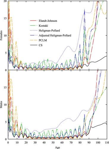
Figure 1 compares the mean loss by age from the CS method with that of the five alternative methods. For Kostaki’s (2000) relational method, we used the extended Coale–Demeny West model life table (UN 2011) as the standard, with $e_0=74$ for females and $e_0=66$ for males (the median life expectancies for respective test sets). For the CS method, we used a constant value of N  =  500,000 for each age interval, on average the value for a population the size of Australia. For Rizzi et al.’s (2015) Penalized Composite Link Model (PCLM) method, we used linear P-splines, a quadratic penalty optimized using the Akaike Information Criterion (Akaike 1974), and a population exposed to the risk of dying given by a stationary distribution with total number 12.5 million, approximately the number of females/males in a population the size of Australia. Following Rizzi et al. (2015), we spaced spline knots one year apart, from age 0 to age 110. The results show that apart from Heligman–Pollard, the methods are equally accurate over the age range 20 to 80. Below age 20 the accuracy of Elandt-Johnson, PCLM, and Kostaki begins to degrade, while Heligman–Pollard shows relative improvement. Kostaki’s (1991) adjusted Heligman–Pollard model improves the parametric fit by adjusting the force of mortality in each age interval to exactly match the observed abridged rate. The CS method is as accurate as adjusted Heligman–Pollard below age 20 and more accurate than Elandt-Johnson and PCLM at ages below five. The CS method is much more accurate than the five alternatives for ages over 95.

Figure 1 Mean loss by age (females and males) for five-year abridged schedules derived from the test set, $\mathrm{H}\mathrm{M}{\mathrm{D}}_t$, using six different methods

Note: Mean loss is calculated using equation (17)(17) $\begin{array}{rl}{ϵ}_l(x)& \\ & :=50\times 100\times {ϵ}_d(x)+25\times 10\times {ϵ}_a(x)\\ & +25\times {ϵ}_r(x),\end{array}$(17) . Source: Based on HMD (2016) data.

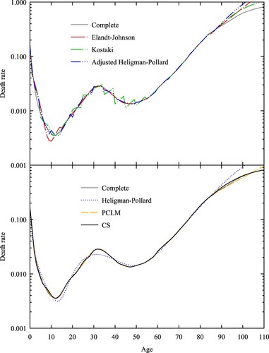
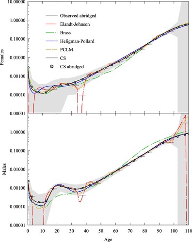
Figure 2 is an illustrative example of the strengths and weaknesses of the six methods. We used the death rates of Italian males for the year 1919, because this is an example where the canonical features of all-cause human mortality described in the Introduction are prominent: the high level of mortality in the first year of life, the rapid decline thereafter, an accident peak, the exponential rise in rates as adults age, and the decrease in the slope for advanced years. Figure 2 shows the expanded schedules for each method alongside the complete schedule from which the abridged rates were derived. The deterioration of Elandt-Johnson for young ages is a common feature of polynomial methods, which struggle to approximate the rapid decline in mortality rates over ages 0–15. As pointed out by Thatcher et al. (1998), the poor performance of Heligman–Pollard, adjusted Heligman–Pollard, and Elandt-Johnson over the open interval is related to the underlying models used by these methods (Heligman–Pollard and Gompertz, respectively), which overestimate the increase in mortality with age. This is also a feature of the PCLM method’s use of a quadratic penalty. Also evident in Figure 2 is a feature of both Kostaki and adjusted Heligman–Pollard that can lead to implausible changes in rates: when the underlying mortality curve (the standard in the case of Kostaki or the Heligman–Pollard model in the case of adjusted Heligman–Pollard) is not a good fit, then the death rates of the adjusted curve will be discontinuous at the abridged age boundaries. In contrast, CS shows good agreement with the complete schedule across all ages.

Figure 2 Death rates for Italian males in 1919: six expansion methods, five-year abridgement

Note: The death rate scale is logarithmic. Source: As for Figure 1.

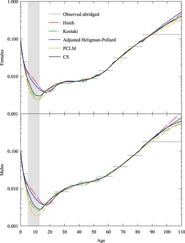
Next, we consider the performance of the methods when the abridgement width increases and the sequence of closed age intervals is truncated at a lower age. For each smoothed schedule in the $\mathrm{H}\mathrm{M}{\mathrm{D}}_t$ data set, we constructed an abridged curve consisting of ages 0, 1, 5 and thereafter ages at 10-year intervals up to 65, with a final open interval of 75 and over. We could not use the Elandt-Johnson method, because it assumes the classic five-year abridgement structure. We used instead Hsieh’s (1991) interpolation method based on cubic splines, because it does not assume a particular abridgement structure. Similar to Elandt-Johnson, it extrapolates into the open interval using the Gompertz model, but it differs in that it also uses a parametric fit for young ages. In our implementation, we used the infant component from de Beer and Janssen’s (2016) CoDe (Compression and Delay) model to fit the first two death rates.

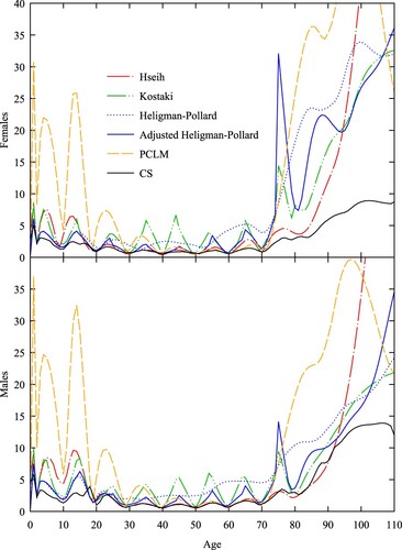
As before, Figure 3 compares the mean loss by age for CS with that of the five alternative methods. However, for the CS method we used a constant value N  =  1,000,000 to account for the doubling of the age interval. The results show that apart from PCLM, the methods are equally accurate over the age range 20–70. Below age 30, the accuracy of PCLM begins to degrade. Below age 20, the accuracy of Hsieh also deteriorates but not to the same extent as PCLM or Elandt-Johnson in Figure 1. There is a large spike in loss for adjusted Heligman–Pollard at the beginning of the open interval in the test sets for both females and males and a rapid increase in the loss for PCLM. The CS method is never less accurate than the three interpolation methods and PCLM, is more accurate than adjusted Heligman–Pollard at the beginning of the open interval and more accurate than Hsieh after age 90.

Figure 3 Mean loss by age (females and males) for 10-year abridged schedules derived from the test set, $\mathrm{H}\mathrm{M}{\mathrm{D}}_t$, using six different methods

Note: Mean loss is calculated using equation (17)(17) $\begin{array}{rl}{ϵ}_l(x)& \\ & :=50\times 100\times {ϵ}_d(x)+25\times 10\times {ϵ}_a(x)\\ & +25\times {ϵ}_r(x),\end{array}$(17) . Source: As for Figure 1.

Figure 4 reprises Figure 2 using 10-year abridged data. We see that Hsieh’s spline struggles to reproduce the profile below age 20 correctly. The discontinuities in Kostaki’s relational method are larger, whereas the two parametric methods and CS show less change relative to their fits to the five-year data. The performance of the five methods over the open interval starting at age 75 is similar to that shown in Figure 2, with PCLM extrapolating with a linear profile and the remaining methods apart from CS tending to overestimate rates after age 90.

Figure 4 Death rates for Italian males in 1919: six expansion methods, 10-year abridgement

Note: The death rate scale is logarithmic. Source: As for Figure 1.

Application of the CS method

We now move on to demonstrating the application of the CS method to other sources of incompleteness in mortality data encountered by demographers. These include the potential unreliable nature of census and vital registration data, a lack of complete publicly available data (as opposed to data held by national statistical offices), and the random timing of death events when the population of interest is sufficiently small. In this section we provide the reader with three applications of the CS method to expanding both five- and 10-year schedules that collectively display inaccuracies (both systematic and random) in rates, discontiguous age intervals (from data that have been excluded as unreliable), and truncation.

Iceland: High sampling noise

The HMD data for Iceland provide an excellent testing ground for CS. The raw data are of high quality and cover the years 1838–2013, during which life expectancy at birth for males and females combined increased from 32 to 82. Although Iceland’s total population increased by a factor of six from 57,000 to 330,000, the concurrent decline in mortality rates means that sample noise continues to be an issue and is the reason Iceland was excluded from the calibration set. Using the standard Poisson approximation to the binomial distribution, we know that for a population, ${}_n{N}_x$, statistical variation of the observed death rate will be less than one significant figure if the underlying death rate, ${}_n{m}_x$, satisfies the inequality (19) ${}_n{m}_x>{\displaystyle \frac{100}{{}_n{N}_x}.}$(19) Figure A4 (supplementary material) compares Iceland’s population pyramids for the years 1868 and 2001. Iceland in 1868 was in its pre-transition stage. Even though death rates were high, we can see that since five-year bucketed populations above age 80 are below 1,000, the corresponding raw death rates will show a high degree of statistical noise. By 2001 Iceland had transitioned to a low-mortality country. The five-year bucketed populations below age 40 for each sex are all approximately 10,000. Therefore, raw mortality rates will show significant statistical noise for rates below 0.01.

Figures 5 and 6 show the raw five-year death rates (horizontal lines) for Iceland in the years 1868 and 2001, respectively, together with the corresponding fits using the Elandt-Johnson spline method, the Brass (1971) relational method, and the Heligman–Pollard, PCLM, and CS fits, together with the abridged rates implied by the CS fit. Here we used $N$ from HMD (2016) given in Figure A4. The grey region in each plot is the 95 per cent confidence interval, assuming that deaths are binomial and the death rate is given by the CS method. As expected, observed death rates are highly variable in 1868 for ages above 80 and in 2001 for ages below 40. In particular, these two years are examples of when a death rate was zero (rates ${}_5{\tilde{m}}_{95}$ for both females and males in 1868; ${}_4{\tilde{m}}_1$ for females and ${}_5{\tilde{m}}_5$ for males in 2001). The CS fits give a reasonable shape despite the presence of zero rates, and any variation from the raw data is well explained by sample variance. For the Elandt-Johnson spline method, we needed to remove the zero death rates for the method to converge. For the Heligman–Pollard fits, it was necessary to change the fitting metric from the sum of squared relative errors to a Poisson log likelihood to model observed rates of zero better. For the Brass fit, we used a standard given by the Coale–Demeny West extended model life table, with life expectancy $e_0=38$ for females and $e_0=30$ for males (Li and Gerland 2011; UN 2011) for 1868, and we used the Coale–Demeny North model with life expectancy $e_0=82$ for females and $e_0=78$ for males for 2001.

Figure 5 Death rates for females and males, Iceland, 1868: five expansion methods and abridged CS rates compared with observed abridged rates

Notes: Grey area refers to 95 per cent confidence interval for abridged rates (which are shown by horizontal lines). Coale–Demeny West model life tables with $e_0=38$ for females and $e_0=30$ for males were used as standards for the Brass relational method. The death rate scale is logarithmic. Source: As for Figure 1.

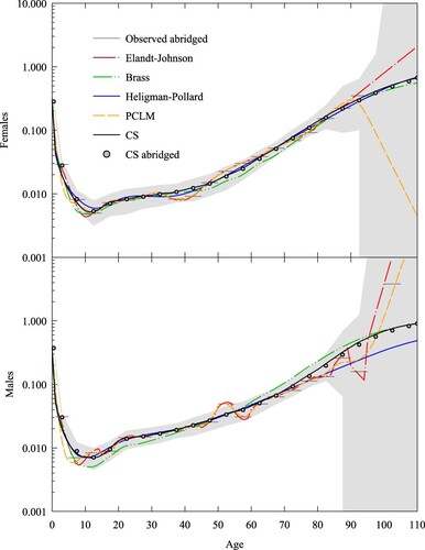
Figure 6 Death rates for females and males, Iceland, 2001: five expansion methods and abridged CS rates compared with observed abridged rates

Notes: Grey area refers to 95 per cent confidence interval for abridged rates (which are shown by horizontal lines). Coale–Demeny North model life tables with $e_0=82$, for females and $e_0=78$ for males were used as standards for the Brass relational method. The death rate scale is logarithmic. Source: As for Figure 1.

To measure the goodness of fit for each method, we used the Poisson deviance (20) $\mathrm{d}\mathrm{e}\mathrm{v}=2\sum _i{N}_i\left[{\tilde{m}}_i\mathrm{l}\mathrm{o}\mathrm{g}\left({\tilde{m}}_i/m_i\right)-\left({\tilde{m}}_i-m_i\right)\right].$(20) Table 1 gives the values for $\mathrm{d}\mathrm{e}\mathrm{v}$ for the four sets of abridged rates. We discounted Elandt-Johnson because three of the four complete schedules were not plausible and two gave negative death rates. PCLM shows the lowest deviances of the four remaining methods but for advanced ages gives death rate slopes that are implausibly high (males, Figures 5 and 6) or even negative (females, Figure 5). This is a result of the penalty term used by PCLM, which is based on a second-order difference, implying that across ages where exposure numbers are low, the model will tend to fit observed rates with an exponential profile in age (or a linear profile when rates are plotted on a logarithmic scale), making the profile sensitive to cases where the last observed rate is unusually low (${}_5{\tilde{m}}_{95}$ for females in Figure 5) or high (${}_5{\tilde{m}}_{100}$ and ${}_5{\tilde{m}}_{105}$ for males in Figures 5 and 6, respectively) as a result of sample noise. We see that Brass provides the worst fit of the four methods. Heligman–Pollard and CS display similar values: HP has a lower value in only one of the four cases.

Table 1 Summary statistics for four expansion methods applied to five-year abridged death rates for females and males in Iceland, 1868 and 2001

Year	Sex	$\mathrm{d}\mathrm{e}{\mathrm{v}}_B$	$\mathrm{d}\mathrm{e}{\mathrm{v}}_{HP}$	$\mathrm{d}\mathrm{e}{\mathrm{v}}_{PCLM}$	$\mathrm{d}\mathrm{e}{\mathrm{v}}_{CS}$
1868	Females	38	12	4	13
1868	Males	137	27	7	25
2001	Females	79	27	12	19
2001	Males	319	24	6	24

Note: Goodness-of-fit measure $\mathrm{d}\mathrm{e}\mathrm{v}$ is the Poisson deviance given by equation (20)(20) $\mathrm{d}\mathrm{e}\mathrm{v}=2\sum _i{N}_i\left[{\tilde{m}}_i\mathrm{l}\mathrm{o}\mathrm{g}\left({\tilde{m}}_i/m_i\right)-\left({\tilde{m}}_i-m_i\right)\right].$(20) . $B$ = Brass; $HP$ = Heligman–Pollard; $PCLM$ = Penalized Composite Link Model; $CS$ = calibrated splines.

Source: Based on HMD (2016) data.

Burkina Faso: Problematic age heaping and missing data

Grouping ages is a method sometimes used to reduce the effects of age heaping: the tendency of reported ages to cluster at certain multiples (Hobbs 2004). Burkina Faso is a West African nation with a fast-growing population of just over 20 million, with relatively high mortality rates. Figure A5 (supplementary material) shows the population pyramid from the Burkina Faso 2006 Population and Housing Census conducted by the Institut National de la Statistique et de la Démographie. We see, superimposed on a young, pre-transition age profile, age heaping at multiples of five and 10, although the former is less pronounced than the latter.

In analysing the death rates of Burkina Faso, Ouedraogo (2020) used non-standard five-year age groups starting at age 13, to reduce the effect of five-year age heaping; however, the data still retained signs of 10-year age heaping. Furthermore, death rates below age 13 were excluded from that analysis because of the under-enumeration of children. To reduce the effect of 10-year age heaping, we aggregated the five-year grouped death and exposure data corrected for census coverage and incompleteness of deaths by Ouedraogo (2020) and supplemented the death rates with infant and child mortality rates from the United Nations Inter-agency Group for Child Mortality Estimation (IGME 2021). The result is a non-contiguous, abridged schedule with age intervals [0,1), [1,5), and 10-year intervals starting at age 13 and terminated by an open interval at age 83.

We supposed that the abridged rates were accurate and chose spline, relational, and parametric methods that recovered the abridged rates. Figure 7 shows the abridged rates and five methods for generating a complete schedule: Hsieh’s (1991) spline method, Kostaki’s (2000) relational method, adjusted Heligman–Pollard, PCLM, and CS. For CS, the abridged population exposed to the risk of dying, N, was taken from Ouedraogo (2020). We also highlight in grey the age range where death rates were excluded. We fitted the relational method using the iterative procedure given in the Appendix and a standard given by the United Nations General extended model life table, with life expectancy $e_0=54$ for females and $e_0=49$ for males (Li and Gerland 2011; UN 2011). We see the schedules fall into two groups over the 5–12 year age range, with spline and parametric methods giving higher rates than the relational, PCLM, and CS methods.

Figure 7 Death rates for females and males, Burkina Faso 1996–2006: five expansion methods compared with observed abridged rates

Notes: Kostaki uses United Nations General model life table ($e_0=54$ for females, $e_0=49$ for males) as standard. Grey area refers to age range without reliable death rates. Abridged rates are shown by horizontal lines. The death rate scale is logarithmic. Source: Based on data from IGME (2021) and Ouedraogo (2020).

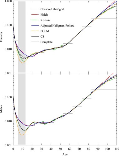
As a validation step, we constructed a censored abridged schedule with the same age intervals as for Burkina Faso, using a complete set of rates taken from the $\mathrm{H}\mathrm{M}{\mathrm{D}}_t$ test set used in the previous section. As test schedules we used the death rates for females and males in Norway in 1859, because Norway then and Burkina Faso in 1996–2006 displayed similar life expectancies. The results are shown in Figure 8, with the censored ages highlighted in grey. The complete schedules are similar to those in Figure 7 and suggest that relational, PCLM, and CS profiles are more plausible than the spline and parametric ones because they more closely correspond to the complete set of rates for Norway.

Figure 8 Death rates for females and males, Norway 1859: five expansion methods compared with censored abridged rates and complete rates

Note: Grey area refers to age range where death rates have been censored. Abridged rates are shown by horizontal lines. The death rate scale is logarithmic. Source: As for Figure 1.

Australian overseas-born residents: Sampling noise and truncation

In 2016 around 26 per cent of Australia’s population was born overseas, up from 22 per cent 10 years prior (ABS 2017). Figure A6 (supplementary material) shows the population pyramid for overseas-born Australian residents in 2019 (ABS 2019a). The data are divided into five-year age intervals terminated by an open interval at age 75. The profile is an inverted version of the 2001 pyramid for Iceland given in Figure A4, reflecting the combined age dependence of immigration intensity and time exposed to the risk of migrating to Australia.

The Australian Bureau of Statistics publishes data on deaths by sex and country of birth at 10-year age intervals terminated by an open interval at age 85 (ABS 2019b). From death and resident population data, we were able to construct a set of abridged death rates for overseas-born Australian residents at 10-year age intervals with an open interval at age 75. The healthy migrant effect (the tendency of death rates for migrants to be lower than for non-migrants [Singh and de Looper 2002; Baffour and Raymer 2019]) and the inverted exposure pyramid together imply that sample noise will be relatively more significant for young ages. We also note that the open interval starts below the life expectancy of overseas-born Australian residents (91 for females and 87 for males in 2019) and hence truncation is significant for this population, with a single rate spanning 90 and 82 per cent of the death distributions for females and males, respectively. Figure 9 shows abridged and complete curves from five expansion methods: Hsieh, Heligman–Pollard, Brass, PCLM, and CS, as well as the abridged rates implied by the CS fit and the CS fit to data for Australian-born residents. Here we used $N$ from the population pyramid given in Figure A6. For Hsieh’s spline method, we needed to remove the zero death rates (${\tilde{m}}_0$ for females and males and ${}_4{\tilde{m}}_1$ for females) for the method to converge. For Brass, we used the corresponding complete set of death rates for Australian-born residents as the standard. For the Heligman–Pollard fits, we used the Poisson log-likelihood as the fitting metric to model observed rates of zero better. In the case of CS, the infant death rate was calculated as the limit in $m_x$ as $x\to 0$. This limit was calculated by fitting the CS values for $x>0$ using the Heligman–Pollard method and taking the value at age 0. Figure 9 also includes for comparison the CS estimate of the complete schedule of death rates for Australian-born residents. The grey region in each plot is the 95 per cent confidence interval assuming that deaths are binomial and the death rate is given by the CS method.

Figure 9 Death rates for female and male overseas-born Australian residents, 2019: five expansion methods, abridged CS rates, and CS fitted to Australian-born residents, compared with observed abridged rates

Notes: CS-AUS refers to CS fit to data for Australian-born residents. Grey area refers to 95 per cent confidence interval for abridged rates (which are shown by horizontal lines). Brass uses the CS fit to Australian-born death rates as standard. The death rate scale is logarithmic. Source: Based on data from ABS (2019a, 2019b).

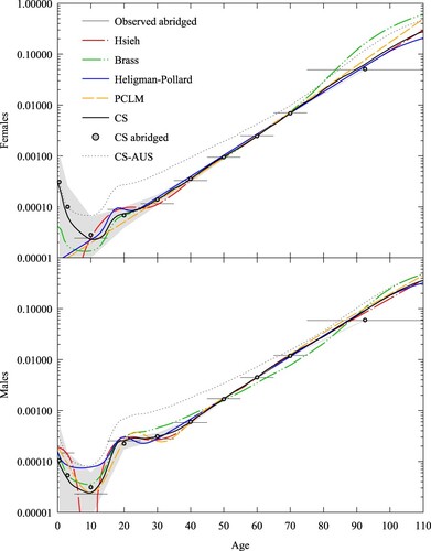
We see from Figure 9 that Brass and CS give reasonable profiles where sample noise is large (ages below 20), and Hsieh, Heligman–Pollard, PCLM, and CS give reasonable profiles when sample noise is small (at ages above 60). Below age 20, Heligman–Pollard and PCLM give implausible profiles of death rates for females, and Hsieh gives negative death rates for both sexes. As discussed in the Iceland subsection, PCLM’s second-order difference penalty leads to it extrapolating log death rates linearly across ages where exposure numbers are small, in this case leading to a linear profile for female children. Above age 60, Brass is biased downward for the rates centred at ages 60 and 70 for males and biased upward for the rate spanning the open interval for females. Table 2 shows the Poisson deviance for each method (other than Hsieh, which we excluded as implausible), split into the deviance of all abridged rates and the deviance for all closed age intervals (i.e. excluding the open interval). We see that PCLM exhibits the smallest deviance over the closed intervals, followed by CS. CS shows the smallest deviance over all intervals in the schedule for males, but for females Heligman–Pollard fits the open interval better and shows the smallest total deviance. The demographer will need to choose either a good fit and a plausible profile (CS) or the best fit and an implausible profile (Heligman–Pollard and PCLM).

Table 2 Summary statistics for four expansion methods applied to 10-year abridged death rates for female and male overseas-born Australian residents in 2019

Sex	Intervals	$\mathrm{d}\mathrm{e}{\mathrm{v}}_B$	$\mathrm{d}\mathrm{e}{\mathrm{v}}_{HP}$	$\mathrm{d}\mathrm{e}{\mathrm{v}}_{PCLM}$	$\mathrm{d}\mathrm{e}{\mathrm{v}}_{CS}$
Females	All	1,839	21	174	30
Males	All	906	54	123	16
Females	Closed	15	18	10	11
Males	Closed	905	41	5	8

Note: Goodness-of-fit measure $\mathrm{d}\mathrm{e}\mathrm{v}$ is the Poisson deviance given by equation (20)(20) $\mathrm{d}\mathrm{e}\mathrm{v}=2\sum _i{N}_i\left[{\tilde{m}}_i\mathrm{l}\mathrm{o}\mathrm{g}\left({\tilde{m}}_i/m_i\right)-\left({\tilde{m}}_i-m_i\right)\right].$(20) . $B$ = Brass; $HP$ = Heligman–Pollard; $PCLM$ = Penalized Composite Link Model; $CS$ = calibrated splines.

Source: Based on data from ABS (2019a, 2019b).

Discussion and conclusion

In this paper we have outlined the new application of the CS method to solving the problem of expanding a set of abridged death rates to give a method that is accurate and robust in the presence of large abridgement intervals, truncation, sample noise, and missing data. Our applied work in the case studies of Iceland, Burkina Faso, and overseas migrants to Australia suggests that the method is a useful addition to existing tools for estimating mortality under these circumstances, especially for nations with small populations (e.g. Iceland), countries with incomplete vital statistics (e.g. Burkina Faso), and subnational populations (e.g. the overseas-born population in Australia). More broadly, our approach illustrates the application of historical data in demographic collections to improve the estimation of key rates by including domain-specific penalties into a non-parametric framework.

Our findings on the comparative accuracy of current methods help to demonstrate the value of our novel application of the CS method and are in line with existing literature. Kostaki and Panousis (2001) compared spline, parametric, and relational methods for expanding abridged death probabilities for the classic five-year structure (0, 1–4, and five-year intervals thereafter). They, too, noted that spline methods, while able to reproduce the observed rates exactly, sometimes showed implausible oscillations for ages below 20; in addition, pure parametric methods guaranteed smooth results, whereas adjusted parametric and the Kostaki relational methods gave more accurate results but at the expense of smoothness (see our Figures 2 and 4). Baili et al. (2005) compared two spline (including Elandt-Johnson) and two relational (Kostaki and Brass) methods for expanding death probabilities with the classic five-year structure up to the 95–99 age group for the purpose of calculating relative survival fractions for cancer patients. Our Figure 1 is consistent with their conclusion that over the age range 20–99, Elandt-Johnson was the preferred method for national populations.

We used principal components to span the range of historical mortality profiles of multiple populations with weights chosen to fit an abridged schedule. This differs from the approach of Lee and Carter (1992) in mortality projections, where the calibration set is the mortality experience of a single population over time and the trend index weights the first principal component of deviations from the time-averaged level. Alexander et al. (2017) also used principal components to estimate subnational death rates, although their focus was on improving estimates of abridged rates using a hierarchical Bayesian framework, whereas ours was on expanding abridged rates. Our approach is more closely related to that of INDEPTH Network (2002), who used principal components to analyse the variation in death probabilities across Africa and Asia, and to that of Clark (2019), who applied them to HMD data as part of a framework for inferring a complete mortality schedule from a general set of covariates, illustrating the approach by constructing models to infer schedules from a single covariate (child mortality, ${}_5{q}_0$) or two covariates (child mortality, ${}_5{q}_0$, and adult mortality, ${}_{45}{q}_{15}$). A benefit of the CS approach is its additional flexibility in allowing deviations from the shapes spanned by the principal components, provided there is a compensating improvement in the fit.

Our use of five principal components to model mortality variation differs from other studies that have used just three (Alexander et al. 2017). Our data set was constructed to encompass the widest possible range of mortality variations in both historical (an average of 85 years per country in the HMD subset) and geographical dimensions (192 countries for the year 2000 in the WHO subset). In contrast, for example, Alexander et al.’s (2017) data set of United States (US) mortality spanned 31 years (1980–2010) and 50 states of a developed country. If we look at life expectancy alone, for our data set the interquartile range was 14.8 compared with 2.8 for the US states, a factor of five difference. Accordingly, when we performed a singular value decomposition of Alexander et al.’s (2017) US data set, we found that three factors were sufficient to account for 95 per cent of the variation in death rates, whereas five were required in ours.

Non-parametric approaches to mortality estimation have been applied to the problem of smoothing death rates (Peristera and Kostaki 2005; Kostaki et al. 2011; de Beer 2012; Gonzaga and Schmertmann 2016), but we are not aware of any approaches other than PCLM and CS in which they have been applied to expanding abridged schedules. CS’s use of a shape penalty term can be seen as an example of Schmertmann’s (2021a) D-spline approach, where B-spline penalties are motivated by desired demographic properties in contrast to P-splines’ use of smoothness penalties (Eilers and Marx 1996; Rizzi et al. 2015). This is significant because smoothness alone is not a sufficient condition for generating profiles that are demographically plausible. Our method differs from that of Schmertmann (2021a) in a number of important ways. Our model focuses on expanding abridged rates, whereas Schmertmann’s (2021a) method is used for smoothing otherwise complete schedules. The former is an example of an underdetermined problem (there are fewer observations than parameters, $g<k$ in our notation), whereas the latter is an overdetermined problem (there are more observations than free parameters, $g>k$). Another difference is that in our model we base penalties on the distance in column space of principal components derived from data from both HMD and WHO, covering all regions of the world. In contrast in Schmertmann (2021a) the penalties are derived from other measures, such as the failure to match differences in rates across successive ages for HMD data only. The application domains of the two methods are also significantly different, with Schmertmann (2021a) applying his method to small populations where sample noise was significant, while our method was applied to larger populations where the problems included sample noise, large abridgement intervals, missing data, and truncation.

This paper has shown how the core elements of the CS method for fertility can be worked into improving mortality schedules, despite the significant differences in the way these two processes are modelled. In Schmertmann (2014), the fertility rate is a linear function of the B-spline weights and the variance of the fitting errors is independent of the rate, which leads to a linear equation for the optimal spline weights. In contrast, in the CS method, the force of mortality is a non-linear function (an exponential) of the B-spline weights, death rates are a non-linear function of the force of mortality, the variance of the fitting errors is proportional to the death rate, and the optimal spline weights satisfy a system of non-linear equations. Despite these differences, we have shown that the spline weights can be found using linear methods via iteration. We have implemented our method as an Excel add-in for readers; this is provided together with data and calculations for examples in the Applications section (see Note 3).

Another novel feature of our approach is the use of the force of mortality, $\mu$, in the calibration and fitting stages; this contrasts with some other approaches, for example Rizzi et al. (2015), who used the death rate. Our motivation for doing this was to create a framework that was extensible. For example, one possible extension would be to use the CS approach to expand abridged death probabilities rather than death rates. It is not uncommon for the death rate column to be missing from a published mortality table (see e.g. INDEPTH Network 2002, Table 7.7), and methods (see Kostaki and Panousis 2001 for a review) and software (see UNABR in UN 2013) exist for expanding the table from probabilities instead. The CS approach can be extended to this setting, too, by adapting the fitting process using the link function, converting from force to probability, (21) ${}_n{q}_x=1-\prod _{{}_{x\le k<x+n}}{e}^{-{\mu }_k},$(21) without needing to recalibrate the shape penalty matrix, $Q_s$.

There are some important limitations of the method demonstrated in this paper. The most significant is that it requires a representative data set to calibrate the shape factors. Put another way, CS is less a stand-alone method and more a means of extrapolating from a reference set of curves. This does limit its application to situations where such an extrapolation is justified, and it raises questions about the effect of choosing an inappropriate calibration set, which requires further research but is outside the scope of this study. This also points to opportunities for calibrating shape factors for alternative collections of mortality, such as by cause (Girosi and King 2007), geographic region (Palloni et al. 2014), or subnational administrative division (CHMD 2021; JMD 2021).

In the CS method (and the other methods tested in this paper, other than the relational models), the mortality curves to be expanded are treated in isolation and do not take into account a population’s relationship with its neighbours in time or space that could improve an estimate of its life table. In particular, for estimates of mortality rates for populations in subnational jurisdictions where there is a significant administrative hierarchy that can be exploited, we would expect the accuracy of relational methods such as Brass to improve. There will still be a role for CS in these cases though. For example, Alexander et al.’s (2017) Bayesian hierarchical method could be used to improve the accuracy of abridged death rates, and then CS could be used to expand the rates subject to the Bayesian error estimates. For relational methods, the CS method could be used to build the standard at the highest geographical level. For example, the CS estimates for the death rates of overseas-born Australians could be used as the standard for an estimate of death rates by region of birth.

Another limitation is related to the effective dimension of CS. Since any linear combination of the five principal components will have a zero shape penalty, the effective dimension of the model is at least five. Our study used mortality data for moderate to large populations, but for populations where the abridged data display a very high degree of sample noise it might be difficult to resolve the weights on each component, in which case the model will become over-parameterized and likely start to give implausible profiles. One area for future work, therefore, is to investigate ways in which CS might be stabilized for such populations. Another opportunity for further research is to understand whether and how CS could be modified for graduating death rates, where the abridgement interval n  =  1, to give a method useful for both smoothing and expanding mortality data, since the fitting framework for CS makes no assumptions about the abridgement age interval. Non-parametric methods for expanding mortality schedules remain an active area of research, with recent work extending both the TOPALS smoothing method (Dyrting 2018) and D-splines (Schmertmann 2021b).

Disclosure statement

No potential conflict of interest was reported by the authors.

Notes

1 Please direct all correspondence to Sigurd Dyrting, Charles Darwin University, Ellengowan Drive, Brinkin, NT 0909, Australia; or by email: [email protected]

2 Funding: This research was in part funded by a grant for independent demographic research by the Northern Territory Department of Treasury and Finance.

3 Data availability: An archive containing an implementation of the mortality CS method as an Excel add-in as well as data and calculations for the CS applications are available as an Excel spreadsheet at https://doi.org/10.17605/OSF.IO/NGR8X. The supplementary material contains additional figures for this paper.

Appendix

Solving the CS equations

In equation (9) the $g\times g$ matrix, $V_f$, is the variance of the fitting errors, assumed to be proportional to the death rate and inversely proportional to the population: (22) $V_f\left(\theta \right)=\mathrm{d}\mathrm{i}\mathrm{a}\mathrm{g}\left({\displaystyle \frac{m\left(\theta \right)}{N}}\right).$(22) In the CS method for expanding fertility schedules, a single value for $N$ equal to the average population per age interval was used. Here it is a $g\times 1$ vector specifying the population for each age interval. The second term in equation (9) is the sum of squared shape residuals normalized by the shape covariance calculated from $\theta$ and the $k\times k$ matrix, $Q_s$, (23) $Q_s=B^{\mathrm{\prime }}\cdot {\overline{P}}^{{}^{\mathrm{\prime }}}\cdot V_s^{-1}\cdot \overline{P}\cdot B,$(23) which we get from equations (6)(6) $e=\overline{P}\cdot \mathrm{l}\mathrm{o}\mathrm{g}\mu ,$(6) and (8)(8) $\mathrm{l}\mathrm{o}\mathrm{g}\mu =B\cdot \theta ,$(8) . The minimum of the penalty function given in equation (9)(9) $\mathcal{L}\left(\theta \right)=\left(m\left(\theta \right)-\tilde{m}\right){}^{\mathrm{\prime }}\cdot V_f^{-1}\left(\theta \right)\cdot \left(m\left(\theta \right)-\tilde{m}\right)+\theta {}^{\mathrm{\prime }}\cdot Q_s\cdot \theta ,$(9) occurs at a value of $\theta$ where the partial derivatives are zero (Dennis and Schnabel 1996): (24) ${\displaystyle \frac{\mathrm{\partial }\mathcal{L}}{\mathrm{\partial }\theta }=0.}$(24) Taking the derivative of $\mathcal{L}$ with respect to the spline weights $\theta$ in equation (9)(9) $\mathcal{L}\left(\theta \right)=\left(m\left(\theta \right)-\tilde{m}\right){}^{\mathrm{\prime }}\cdot V_f^{-1}\left(\theta \right)\cdot \left(m\left(\theta \right)-\tilde{m}\right)+\theta {}^{\mathrm{\prime }}\cdot Q_s\cdot \theta ,$(9) , substituting into equation (24)(24) ${\displaystyle \frac{\mathrm{\partial }\mathcal{L}}{\mathrm{\partial }\theta }=0.}$(24) , and taking the transpose gives the non-linear system of equations, (25) $G\left(\theta \right){}^{\mathrm{\prime }}\cdot Q_f\cdot \left(m\left(\theta \right)-\tilde{m}\right)+Q_s\cdot \theta =0.$(25) Our objective is to solve this system of equations for the spline weights, $\theta$. To do this, we first derive formulae for the $g\times 1$ vector, $m\left(\theta \right)$, and the $g\times k$ derivative matrix, $G\left(\theta \right)$, in terms of the spline weights, $\theta$. An element of the vector, $m\left(\theta \right)$, will be a model death rate, ${}_n{m}_x$, for an age interval, $\left[x,x+n\right)$. From equation (8)(8) $\mathrm{l}\mathrm{o}\mathrm{g}\mu =B\cdot \theta ,$(8) it follows that the force of mortality at age $x$ is (26) ${\mu }_x=\mathrm{e}\mathrm{x}\mathrm{p}\left(B_x\cdot \theta \right)$(26) and its $1\times k$ vector derivative with respect to $\theta$ is (27) ${\displaystyle \frac{\mathrm{\partial }{\mu }_x}{\mathrm{\partial }\theta }={\mu }_x{B}_x,}$(27) where $B_x$ is the $x$th $1\times k$ row vector of matrix $B$. Building the survival fraction as a cumulative product of survival probabilities gives expressions (28) $l_x=\prod _{k<x}{e}^{-{\mu }_k}\mathrm{a}\mathrm{n}\mathrm{d}$(28) (29) ${\displaystyle \frac{\mathrm{\partial }{l}_x}{\mathrm{\partial }\theta }=l_x{C}_x}$(29) for the survival fraction and its $1\times k$ derivative, where $C_x$ is the $1\times k$ vector given by the sum (30) $C_x=-\sum _{k<x}{\mu }_k{B}_k.$(30) Using the trapezoidal rule to approximate the integral of the survival fraction gives expressions (31) ${}_n{L}_x=\sum _{x\le k<x+n}\left(l_k+l_{k+1}\right)/2\mathrm{a}\mathrm{n}\mathrm{d}$(31) (32) ${\displaystyle \frac{{\mathrm{\partial }}_n{L}_x}{\mathrm{\partial }\theta }={}_n{D}_x}$(32) for the number of person-years lived and its $1\times k$ derivative, where ${}_n{D}_x$ is the $1\times k$ vector given by the sum (33) ${}_n{D}_x={\displaystyle \frac{1}{2}\sum _{x\le k<x+n}\left[l_k{C}_k+l_{k+1}{C}_{k+1}\right].}$(33) Finally, using the standard expression for the model death rate, (34) ${}_n{m}_x=\left(l_x-l_{x+n}\right){/}_n{L}_x,$(34) and taking the derivative with respect to $\theta$, we obtain the $1\times k$ vector, (35) ${\displaystyle \frac{{\mathrm{\partial }}_n{m}_x}{\mathrm{\partial }\theta }={}_n{G}_x,}$(35) where ${}_n{G}_x$ is the $1\times k$ vector, (36) ${}_n{G}_x={\displaystyle \frac{l_x{C}_x-l_{x+n}{C}_{x+n}}{{}_n{L}_x}-{\displaystyle \frac{{}_n{m}_x}{{}_n{L}_x}{}_n{D}_x.}}$(36) Arranging the $g$ scalars, ${}_n{m}_x$, in a column, we obtain the $g\times 1$ vector, $m\left(\theta \right)$, and arranging the $g$ $1\times k$ row vectors, ${}_n{G}_x$, in a column, we get the $g\times k$ matrix of derivatives, $G\left(\theta \right)$.

Now that we have expressions for $m\left(\theta \right)$ and $G\left(\theta \right)$, the next step is to devise an iterative solution to equation (25). Assume we have an approximate solution, $\overline{\theta }$, that is close to the true solution, $\theta$. Then, using the Taylor series for $m$ at $\overline{\theta }$ taken to first order in $\theta -\overline{\theta }$, the model death rate at $\theta$ will be approximately (37) $m\left(\theta \right)\approx m\left(\overline{\theta }\right)+G\left(\overline{\theta }\right)\cdot \left(\theta -\overline{\theta }\right),$(37) and approximating the derivative matrix by its value at $\overline{\theta }$ (38) $G\left(\theta \right)\approx G\left(\overline{\theta }\right),$(38) and substituting equations (37)(37) $m\left(\theta \right)\approx m\left(\overline{\theta }\right)+G\left(\overline{\theta }\right)\cdot \left(\theta -\overline{\theta }\right),$(37) and (38)(38) $G\left(\theta \right)\approx G\left(\overline{\theta }\right),$(38) into equation (25)(25) $G\left(\theta \right){}^{\mathrm{\prime }}\cdot Q_f\cdot \left(m\left(\theta \right)-\tilde{m}\right)+Q_s\cdot \theta =0.$(25) gives the iteration shown in equation (10)(10) $Q\left(\overline{\theta }\right)\cdot \theta =b\left(\overline{\theta }\right),$(10) .

Fitting the alternative models

The parametric method was calibrated to the observed data by fitting the model death rate, (39) ${}_n{m}_x={\displaystyle \frac{l_x-l_{x+n}}{{}_n{L}_x},}$(39) to the observed death rate, ${}_n{\tilde{m}}_x$, by minimizing the sum of squared relative errors. The spline, relational, and hybrid methods are expressed as interpolations of the survival fraction (or equivalently the death probability). To fit them to death rates, we used the following iterative procedure. Assume an approximate set of survival fractions, ${\overline{l}}_{x+n}$, at the end of each closed interval and person-years lived, ${}_{\mathrm{\infty }}{\overline{L}}_a$, over the open interval. Interpolate these to a complete life table, then calculate updated survival fractions and person-years lived using (40) $l_{x+n}={\overline{l}}_x\mathrm{e}\mathrm{x}\mathrm{p}\left({-}_n{\tilde{m}}_x\times {}_n{\overline{\mathrm{\Delta }}}_x\right)\mathrm{a}\mathrm{n}\mathrm{d}$(40) (41) ${}_{\mathrm{\infty }}{L}_a={\overline{l}}_a{/}_{\mathrm{\infty }}{\tilde{m}}_a,$(41) where (42) ${}_n{\mathrm{\Delta }}_x:={\displaystyle \frac{\mathrm{l}\mathrm{o}\mathrm{g}\left(l_x/l_{x+n}\right)}{{}_n{m}_x}.}$(42) Repeat until ${}_n{m}_x$ equals ${}_n{\tilde{m}}_x$ to the desired precision. The Ansatz equation (40)(40) $l_{x+n}={\overline{l}}_x\mathrm{e}\mathrm{x}\mathrm{p}\left({-}_n{\tilde{m}}_x\times {}_n{\overline{\mathrm{\Delta }}}_x\right)\mathrm{a}\mathrm{n}\mathrm{d}$(40) is motivated by the property that when the force of mortality is constant, ${}_n{\mathrm{\Delta }}_x=n$, so that ${}_n{\mathrm{\Delta }}_x$ is only weakly dependent on $l_{x+n}$ and plays the role of a pseudoconstant in the iteration (Acton 1996). The non-parametric method, PCLM, was fitted using iteratively reweighted least squares (Rizzi et al. 2015).

References

- Abowd, John, Daniel Kifery, Brett Moran, Robert Ashmead, Philip Leclerc, William Sexton, Simson Garfinkel, et al. 2019. Census TopDown: Differentially private data, incremental schemas, and consistency with public knowledge. Working Paper, U.S. Census Bureau.
- ABS. 2017. 2016 Census of Population and Housing time series profile. Catalogue Number 2003.0, Australian Bureau of Statistics.
- ABS. 2019a. Migration, Australia, 2019. Data Release 3412.0, Australian Bureau of Statistics.
- ABS. 2019b. Deaths, Australia, 2019. Data Release 3302.0, Australian Bureau of Statistics.
- Acton, Forman S. 1996. Real Computing Made Real. Princeton: Princeton University Press.
- Akaike, H. 1974. A new look at the statistical model identification, IEEE Transactions on Automatic Control 19(6): 716–723. https://doi.org/10.1109/TAC.1974.1100705
- Alexander, Monica, Emilio Zagheni, and Magali Barbieri. 2017. A flexible Bayesian model for estimating subnational mortality, Demography 54(6): 2025–2041. https://doi.org/10.1007/s13524-017-0618-7
- Arunachalam, D. 2004. Reproductivity, in J. S. Siegel and D. A. Swanson (eds), The Methods and Materials of Demography, 2nd ed San Diego: Elsevier Academic Press, pp. 429–453.
- Baffour, Bernard, and James Raymer. 2019. Estimating multiregional survivorship probabilities for sparse data: An application to immigrant populations in Australia, 1981–2011, Demographic Research 40(18): 463–502. https://doi.org/10.4054/DemRes.2019.40.18
- Baili, P., A. Micheli, A. Montanari, and R. Capocaccia. 2005. Comparison of four methods for estimating complete life tables from abridged life tables using mortality data supplied to EUROCARE-3, Mathematical Population Studies 12: 183–198. https://doi.org/10.1080/08898480500301751
- Blake, David, and Andrew J. G. Cairns. 2021. Longevity risk and capital markets: The 2019–20 update, Insurance: Mathematics and Economics 99: 395–439. https://doi.org/10.1016/j.insmatheco.2021.04.001
- Brass, William. 1971. On the scale of mortality, in W. Brass (eds), Biological Aspects of Demography (Vol. 10). London: Taylor & Francis, pp. 69–110.
- Chiang, Chin Long. 1984. The Life Table and its Applications. Malabar: Robert E. Krieger Publishing Company.
- CHMD. 2021. Canadian Human Mortality Database. Department of Demography, Université de Montréal (Canada). Available: http://www.bdlc.umontreal.ca/chmd/.
- Clark, Samuel J. 2019. A general age-specific mortality model with an example indexed by child mortality or both child and adult mortality, Demography 56: 1131–1159. https://doi.org/10.1007/s13524-019-00785-3
- Coale, Ansley J., and Paul Demeny. 1966. Regional Model Life Tables and Stable Populations. Princeton: Princeton University Press.
- CSDH. 2008. Closing the gap in a generation: Health equity through action on the social determinants of health. Final report of the commission on social determinants of health. World Health Organization. Retrieved from https://www.who.int/publications/i/item/9789241563703.
- de Beer, Joop. 2012. Smoothing and projecting age-specific probabilities of death by TOPALS, Demographic Research 27(20): 543–592. https://doi.org/10.4054/DemRes.2012.27.20
- de Beer, Joop, and Fanny Janssen. 2014. The NIDI mortality model: A new parametric model to describe the age pattern of mortality. Working Paper 2014/7, Netherlands Interdisciplinary Demographic Institute.
- de Beer, Joop, and Fanny Janssen. 2016. A new parametric model to assess delay and compression of mortality, Population Health Metrics 14. https://doi.org/10.1186/s12963-016-0113-1
- Dennis, Jr, J. E, and Robert B. Schnabel. 1996. Numerical Methods for Unconstrained Optimization and Nonlinear Equations. Philadelphia: Society for Industrial and Applied Mathematics. https://doi.org/10.1137/1.9781611971200.
- Dickson, David C. M., Mary R. Hardy, and Howard R. Waters. 2019. Actuarial Mathematics for Life Contingent Risks, 3rd ed. Cambridge: Cambridge University Press.
- Dyrting, Sigurd. 2018. Penalised TOPALS as a tool for expanding abridged fertility and mortality schedules for small populations. https://doi.org/10.13140/RG.2.2.35835.41764.
- Eilers, Paul H. C., and Brian D. Marx. 1996. Flexible smoothing with B-splines and penalties, Statistical Science 11(2): 89–121. https://doi.org/10.1214/ss/1038425655
- Elandt-Johnson, Regina C., and Norman L. Johnson. 1980. Survival Models and Data Analysis. New York: John Wiley & Sons.
- Fraser, Bruce, and Janice Wooton. 2005. A proposed method for confidentialising tabular output to protect against differencing, Paper presented at Joint UNECE/Eurostat work session on statistical data confidentiality, Geneva, Switzerland, 9–11 November 2005.
- Fries, James F. 1980. Aging, natural death, and the compression of morbidity, New England Journal of Medicine 303(3): 130–135. https://doi.org/10.1056/NEJM198007173030304
- Girosi, Frederico, and Gary King. 2007. Cause of Death Data. Harvard Dataverse. Available: https://doi.org/10.7910/DVN/ZVN8XQ.
- Golub, Gene H., and Charles F. Van Loan. 1996. Matrix Computations, 3rd ed. Baltimore: The John Hopkins University Press.
- Gompertz, Benjamin. 1825. On the nature of the function expressive of the law of human mortality, and on a new mode of determining the value of life contingencies, Philosophical Transactions of the Royal Society of London 115: 513–583. https://doi.org/10.1098/rstl.1825.0026
- Gonzaga, Marcos Roberto, and Carl Schmertmann. 2016. Estimating age- and sex-specific mortality rates for small areas with TOPALS regression: An application to Brazil in 2010, Revista Brasileira de Estudos de População 33(3): 629–652. https://doi.org/10.20947/S0102-30982016c0009
- Graunt, John. 1662. Natural and Political Observations Mentioned in a Following Index, and Made upon the Bills of Mortality. London: Natural and Political Observations.
- Greenwood, Major. 1934. Discussion on Mr. Yule’s paper, Journal of the Royal Statistical Society 97(1): 73–84. https://doi.org/10.1111/j.2397-2335.1934.tb04111.x
- Greville, Thomas N. E. 1948. Mortality tables analyzed by cause of death, Record of the American Institute of Actuaries 37: 283–294.
- Halley, Edmond. 1693. An estimate of the degrees of the mortality of mankind; drawn from curious tables of the births and funerals at the city of Breslaw; with an attempt to ascertain the price of annuities upon lives, Philosophical Transactions of the Royal Society of London 17: 596–610. https://doi.org/10.1098/rstl.1693.0007
- Heligman, L., and J. H. Pollard. 1980. The age pattern of mortality, Journal of the Institute of Actuaries 107(1): 49–80. https://doi.org/10.1017/S0020268100040257
- HMD. 2016. Human Mortality Database. University of California, Berkeley (USA) and Max Planck Institute for Demographic Research (Germany). Available: www.mortality.org or www.humanmortality.de (accessed: 30 March 2016).
- Hobbs, Frank B. 2004. Age and sex composition, in J. S. Siegel and D. A. Swanson (eds), The Methods and Materials of Demography, 2nd ed San Diego: Elsevier Academic Press, pp. 125–173.
- Hsieh, John J. 1991. Construction of expanded continuous life tables – a generalization of abridged and complete life tables, Mathematical Biosciences 103: 287–302. https://doi.org/10.1016/0025-5564(91)90057-p
- IGME. 2021. UN inter-agency group for child mortality estimation. Available: https://childmortality.org (accessed: 18 March 2021).
- INDEPTH Network. 2002. Population and Health in Developing Countries, Volume 1: Population, Health, and Survival at INDEPTH Sites. Ottawa: International Development Research Centre.
- JMD. 2021. Japanese Mortality Database. National Institute of Population and Social Security Research. Available: http://www.ipss.go.jp/p-toukei/JMD/index-en.asp.
- Kostaki, Anastasia. 1991. The Heligman-Pollard formula as a tool for expanding an abridged life table, Journal of Official Statistics 7(3): 311–323.
- Kostaki, Anastasia. 2000. A relational technique for estimating the age-specific mortality pattern from grouped data, Mathematical Population Studies 9(1): 83–95. https://doi.org/10.1080/08898480009525496
- Kostaki, Anastasia, Javier M. Moguerza, Alberto Olivares, and Stelios Psarakis. 2011. Support vector machines as tools for mortality graduation, Canadian Studies in Population 38: 37–58. https://doi.org/10.25336/P6VS46
- Kostaki, Anastasia, and Vangelis Panousis. 2001. Expanding an abridged life table, Demographic Research 5: 1–22. https://doi.org/10.4054/demres.2001.5.1
- Lee, Ronald D., and Lawrence Carter. 1992. Modeling and forecasting U.S. mortality, Journal of the American Statistical Association 87(419): 659–671. https://doi.org/10.1080/01621459.1992.10475265
- Li, Nan, and Patrick Gerland. 2011. Modifying the Lee-Carter method to project mortality changes up to 2100, Paper presented at the Population Association of America 2011 Annual Meeting, Washington, DC, 3 March–2 April 2011.
- Makeham, William Matthew. 1860. On the law of mortality and the construction of annuity tables, The Assurance Magazine, and Journal of the Institute of Actuaries 8(6): 301–310. https://doi.org/10.1017/S204616580000126X
- Marmot, Michael. 2015. The Health gap: The Challenge of an Unequal World. London: Bloomsbury.
- NIAA. 2020. Closing the gap: Report for 2020. House Of Reps. Misc. Paper No. 14686, Australian Government National Indigenous Australians Agency.
- Oppermann, Ludvig Henrik Ferdinand. 1870. On the graduation of life tables, with special application to the rate of mortality in infancy and childhood, The Insurance Record. Minutes from a meeting in the Institute of Actuaries, 1 February 1870.
- Ouedraogo, Soumaïla. 2020. Estimation of older adult mortality from imperfect data: A comparative review of methods using Burkina Faso censuses, Demographic Research 43(38): 1119–1154. https://doi.org/10.4054/demres.2020.43.38
- Palloni, Alberto, Guido Pinto-Aguirre, and Hiram Beltrán-Sánchez. 2014. Latin American Mortality Database (LAMBdA). University of Wisconsin. Available: https://www.ssc.wisc.edu/cdha/latinmortality2.
- Peristera, Paraskevi, and Anastasia Kostaki. 2005. An evaluation of the performance of kernel estimators for graduating mortality data, Journal of Population Research 22(2): 185–197. https://doi.org/10.1007/bf03031828
- Preston, Samuel H., Irma T. Elo, and Quincy Stewart. 1999. Effects of age misreporting on mortality estimates at older ages, Population Studies 53(2): 165–177. https://doi.org/10.1080/00324720308075
- Riley, James C. 2005a. Estimates of regional and global life expectancy, 1800–2001, Population and Development Review 31(3): 537–543. https://doi.org/10.1111/j.1728-4457.2005.00083.x
- Riley, James C. 2005b. The timing and pace of health transitions around the world, Population and Development Review 31(4): 741–764. https://doi.org/10.1111/j.1728-4457.2005.00096.x
- Rizzi, Silvia, Jutta Gampe, and Paul H. C. Eilers. 2015. Efficient estimation of smooth distributions from coarsely grouped data, American Journal of Epidemiology 182(2): 138–147. https://doi.org/10.1093/aje/kwv020
- Rizzi, Silvia, Ulrich Halekoh, Mikael Thinggaard, Gerda Engholm, Niels Christensen, Tom Børge Johannesen, and Rune Lindahl-Jacobsen. 2019. How to estimate mortality trends from grouped vital statistics, International Journal of Epidemiology 48(2): 571–582. https://doi.org/10.1093/ije/dyy183
- Rogers, Andrei. 1975. Introduction to Multiregional Mathematical Demography. New York: John Wiley & Sons.
- Schmertmann, Carl. 2014. Calibrated spline estimation of detailed fertility schedules from abridged data, Revista Brasileira de Estudos de População 31(2): 291–307. https://doi.org/10.1590/s0102-30982014000200004
- Schmertmann, Carl. 2021a. D-splines: Estimating rate schedules using high-dimensional splines with empirical demographic penalties, Demographic Research 44(45): 1085–1114. https://doi.org/10.4054/DemRes.2021.44.45
- Schmertmann, Carl. 2021b. D-spline estimation for partial or age-grouped data. https://bonecave.schmert.net/D-splines-with-age-group-data.html.
- Singh, Mohan, and Michael de Looper. 2002. Australian health inequalities: Birthplace. Bulletin No. 2. AIHW Cat. No. AUS 27, Canberra: Australian Institute of Health and Welfare.
- Taylor, Andrew, and Tony Barnes. 2013. “Closing the gap” in Indigenous life expectancies: What if we succeed?, Journal of Population Research 30: 117–132. https://doi.org/10.1007/s12546-013-9106-0
- Thatcher, A. R., V. Kannisto, and J. W. Vaupel. 1998. The Force of Mortality at Ages 80 to 120. Odense: Odense University Press.
- Thiele, T. N. 1871. On a mathematical formula to express the rate of mortality throughout the whole of life, tested by a series of observations made use of by the Danish Life Insurance Company of 1871, Journal of the Institute of Actuaries and Assurance Magazine 16(5): 313–329. https://doi.org/10.1017/s2046167400043688
- Treasury. 2015. 2015 intergenerational report: Australia in 2055. House Of Reps DPL No. 135, Australian Government Treasury.
- UN. 1955. Age and sex patterns of mortality: Model life-tables for under-developed countries. United Nations Publication ST/SOA/SER.A/22, Department of Economic and Social Affairs, Population Branch.
- UN. 1968. The concept of a stable population: Application to the study of populations of countries with incomplete demographic statistics. United Nations Publication ST/SOA/SER.A/39, Department of Economic and Social Affairs.
- UN. 1982. Model life tables for developing countries. United Nations Publication ST/ESA/SER.A/77, Department of International Economic and Social Affairs.
- UN. 1988. MortPak - the United Nations software package for mortality measurement: Batch-oriented software for the mainframe computer. United Nations Publication ST/ESA/SER.R/78, Department of International Economic and Social Affairs.
- UN. 1999. Standard country or area codes for statistical use (M49). United Nations Publication ST/ESA/STAT/SER.M/49/Rev.3,. Retrieved from https://unstats.un.org/unsd/methodology/m49/.
- UN. 2011. Model life tables. United Nations. Available: https://www.un.org/development/desa/pd/fr/node/3294.
- UN. 2012. Changing levels and trends in mortality: The role of patterns of death by cause. United Nations Publication ST/ESA/SER.A/318, Department of Economic and Social Affairs, Population Division.
- UN. 2013. MortPak for Windows: Version 4.3. United Nations Publication POP/SW/MORTPAK/2003, Department of Economic and Social Affairs, Population Division.
- UN. 2022. World population prospects: Summary of results. United Nations Publication DESA/POP/2021/TR/NO. 3, Department of Economic and Social Affairs, Population Division.
- Vaupel, James W. 2010. Biodemography of human ageing, Nature 464: 536–542. https://doi.org/10.1038/nature08984
- Vaupel, James W., Marie-Pier Bergeron-Boucher, and Ilya Kashnitsky. 2021. Outsurvival as a measure of the inequality of lifespans between two populations, Demographic Research S 8(35): 853–864. https://doi.org/10.4054/DemRes.2021.44.35
- WHO. 2016. Global health observatory. World Health Organization. Available: https://www.who.int/data/gho (accessed: 21 April 2016).
- Wilmoth, J. R., K. Andreev, D. Jdanov, and D. A. Glei. 2007. Methods protocol for the Human Mortality Database. Human Mortality Database.