Novel testing device and routine to characterise the spreadability of powders for powder bed fusion processes – a problem-oriented approach

ABSTRACT

Currently there is considerable interest in understanding and quantifying the powder characteristics that affect the quality of the top spread powder layer for processes such as powder bed fusion and binder jetting. For this purpose, a new testing device has been developed in order to assess several aspects of this top spread powder layer. Using different measurement procedures, the roughness of the top layer, the surface coverage of a single spread powder layer and the powder bed density of an entire spreading experiment can be determined. Since the tester is freely programmable, the individual process steps of spreading a single powder layer can also be varied. Using these methods, the influence of different process parameters such as e.g. the spreading velocity or the distance between the blade and the building platform, which is also referred to as gap size in general, on the quality of the top or only a single spread layer and on the powder bed packing density can be examined. This study presents the new test device as well as the corresponding measurement procedures mentioned, the reproducibility of the results, which, depending on the measurement method and the measured parameter, range between 0.24 and 4.81%, and the influence of the spreading strategy, which defines the chronological order of the single steps during spreading.

KEYWORDS:

• Additive manufacturing
• powder bed fusion
• spreading
• spreadability
• testing
• python

1. Introduction

Additive Manufacturing (AM) processes, such as Laser Beam Powder Bed Fusion (LB-PBF) technologies, are characterised by their layer-by-layer build-up, which provides a high degree of design freedom. In order to be able to guarantee a high quality of the part to be printed, it is necessary to highlight and examine all aspects of the AM process steps in the greatest detail. In this connection, one of the most important process steps is exactly the step of applying the powder in this characteristic layer-wise structure, which is also known as spreading. In recent years, there has been an increased awareness of the importance of this step in the process and thus, spreading and all its facets have become increasingly significant. More and more papers are being written about the spreadability of powders and the effects of various recoater blades, different spreading velocities and particle size distributions (PSD) as well as the gap size, to name only a few [1–19].

Like flowability, which should not be mixed up with flow time, spreadability can be regarded as a powder property. The flow time is measured by means of a calibrated so-called Hall funnel (see ISO 4490:2018). The flowability, on the other hand, as a more general term includes several measurable parameters (e.g. flow time, cohesiveness, particle size and shape and other interparticular forces) and describes the complex behaviour of the powder when it moves [20,21]. The spreadability could thus also be subordinated to the flowability, since it involves the agitated spreading of a thin powder layer. Nevertheless, spreadability should be treated as a separate property, especially since it requires other measurable parameters to describe it. If one could now measure the spreadability of a powder for AM techniques, it would already be possible to make a preliminary statement as to whether a powder is suitable for use or not. Owing to the high cost and the long duration of an AM build job, this has always been of particular interest, which is why new testing methods are already available in this field [22–25]. None of the commercially available measuring instruments to date, however, such as the REVOLUTION Powder Analyzer from Mercury Scientific Inc. or the powder rheometer from Anton Paar GmbH to name just two, deal with the spreading of the powder per se, but they attempt to describe its suitability via other measurable powder properties. However, as the quality of a spread powder layer is of crucial importance for a successful build job, the focus of this work was set to assess the quality of such a layer and develop a special testing device as well as various methods to describe spread powder layers. The reproducibility of the obtained results is also discussed in more detail in this study. Since the tester is to be used to investigate the spreading of AM powder in more detail, it has been named Spreading Tester. Using this device, one could try to link the measurable powder properties of the previously mentioned new techniques to the real spreading behaviour of the powders.

2. Materials and methods

2.1. Powder used and basic powder characterisation

For this study, an IN718 superalloy powder grade was used, which was produced by inert gas atomisation, subsequently undergoing additional plasma spheroidisation. Thus, the powder should contain almost exclusively spherical particles. Using this powder, a basic characterisation was performed, determining the Hall flow rate [26], the apparent density, using a funnel [27] as well as an Arnold Meter [28], and the tap density [29]. Each characteristic was measured a total of three times.

Additionally, the shape of the particles was investigated using a JEOL JSM 6490 HV scanning electron microscope (SEM), and the volume-related PSD was measured using a CAMSIZER X2. For the latter, the default settings of the device were used, which means that for the measurement the minimum chord length (x_{c min}) was used for the determination of the particle size of the single particles, and the class width was 1 µm.

2.2. Spreading tester

While those powder characteristics that describe the filling behaviour are also suitable for testing the employability of powders for LB-PBF AM techniques, this does not apply to the flow time. The reason for this is simply that the flowmeter test, which requires the powder to flow through a funnel and is thus better suited to describing the duration of the filling process of a die, does not reflect well the spreading process in LB-PBF AM techniques, where powder is pushed in front of a recoater blade. This has already been shown in several publications which describe that various powders did not flow freely through the Hall funnel, but could be spread – or even processed via selective laser melting (SLM) – without any problems [12,15,30,31]. Owing to the lack of suitable characterisation methods for powders used in LB-PBF AM techniques in the first place, the so-called Spreading Tester was developed, which can be seen in Figure 1. The Spreading Tester is just a miniature 3D printer based on the powder bed fusion technology. In contrast to a real LB-PBF printer it is not operated in an inert atmosphere but instead in ambient air, since it is not encapsulated, and it is not equipped with a laser. Thus, the Spreading Tester is really only designed for powder spreading.

Figure 1. Spreading tester [32].

The Spreading Tester has two Teflon overflow bins, one on each side. This allows excess powder to be collected during and after a spreading test, and since these bins can be easily removed by hand, the powder can be reused afterwards.

The two circular aluminium cylinders in the centre of the Spreading Tester, visible in Figure 1, are the builder and the feeder of the Spreading Tester, whereby the left one was termed as builder and the right one as feeder. During a spreading test, the feeder provides powder that is then spread as a single powder layer in the builder. The complete internal setup can be seen in Figure 2. Inside each of them, there is a Teflon piston, which is driven by a ZSS 25.200.0,6 stepper motor from the company Phytron via a spindle with a pitch of 1 mm. The programming of the motor was finally chosen so that the piston moves at a speed of 1 mm s⁻¹ by default and 0.5 mm s⁻¹ during initialisation. For precise positioning of the Teflon pistons, a linear miniature PCB-level incremental magnetic encoder from the company Renishaw was used. The incremental encoder is a small green circuit board with a black read head that rests against the magnetised tape, which is connected to the piston via a guide. The smallest increment is about 0.488 µm. An additional guide rod attached to the bottom of the piston prevents it from twisting during movement. For the initialisation of the piston, a mechanical limit switch was added, which trips on contact and thereby serves as mechanical zero point. As no mechanical limit switch could be added in the other direction to prevent the piston from moving outside the cylinder, a software limit switch for a specified height was programmed. The maximum stroke of the pistons is 20 mm, which was regarded sufficient for characterising a powder. Once again, both containers (feeder and builder) can be removed from the tester by hand, whereby a special lifting platform was developed for the builder in order to enable removing it from the tester with as little shaking or vibration as possible. In this way, the spread surface in the builder that is to be examined is not changed and the spread powder can also be reused. The lifting platform is driven by a geared motor which thereby elevates the builder with a speed of approximately 2.5 mm s⁻¹ and uses mechanical limit switches to stop at the respective lowest and highest position.

Figure 2. Internal setup of the feeder/builder [32].

The mounted blade is shown enlarged in Figure 3. It is made of high-speed steel (HSS) and has a rhombic profile. To change the blade, only the four screws, two on each side of the blade’s fixation, have to be loosened. This makes it possible to change the blade used for a single spreading test; all that is needed is a corresponding attachment. Such a holder for polymer blades, for example, is sketched in Figure 4. Figure 5 shows a few examples of blades that can be mounted and used on the Spreading Tester. Also, the mounted blade is operated by a stepper motor that is linked to the blade through a gear belt. Spreading velocities of up to 500 mm s⁻¹ are possible thanks to the gear transmission ratio and the torque of the stepper motor. For the initialisation of the blade, magnetic limit switches are located at the height of the overflow bins in both directions of movement, which are triggered without contact as soon as the blade is in front of them. During initialisation, the speed of the blade is limited to 50 mm s⁻¹. This limit switches also prevent the blade from moving out of range.

Figure 3. Mounted blade [32].

Figure 4. Attachment for polymer blades [32].

Figure 5. Mountable blades (1 and 2: polymer blades with different shapes; 3: HSS blade with rhombic shape) [32].

The entire Spreading Tester, except the lifting platform, is controlled by a Phytron phyMOTION freely programmable motion controller (PMC) for multi-axis stepper motor applications. In total three different axes are being used to control the blade, builder and feeder. The lifting platform, on the other hand, is controlled by a DLP-IOR4 module latching relay. Both devices are connected to the computer via USB. Thus, LabVIEW programs were written for different testing procedures. The first program that was written had the purpose to control each motor individually and was therefore also called ‘Direct Mode’. The second and third programs were written to perform various spreading test sequences, one inspired by an EOS and the other by a Concept Laser machine, which mainly differ in their spreading routine (see below). However, it is identical in both test programs that powder is first provided by the feeder, which is why this is not specifically mentioned below.

In Figure 6 the spreading routine inspired by the EOS machine is shown. At the beginning (1), the build platform, which in the case of the Spreading Tester is called piston, is moved down and the layer thickness is set accurately. Then (2) the powder is spread on the building platform by the forward movement of the blade. In the real LB-PBF process, the freshly spread powder layer would now be selectively melted. In the next step (3), this freshly spread powder is protected from effects by the blade by the building platform moving downward before the blade finally drives back to its initial position.

Figure 6. Simplified spreading routine inspired by an EOS machine [12].

The spreading routine inspired by the Concept Laser machine is shown in Figure 7. First (1), the building platform is moved down by a certain percentage further than the actual layer thickness. In the next step (2), the blade is moved forward and spreads the powder on the building platform. Now (3), the specified layer thickness is precisely adjusted by the building platform moving up by a defined margin. At the end (4), excess powder on the building platform is wiped off by the blade driving back to its initial position with its sloping side. In the real LB-PBF process, the freshly spread powder layer would now be selectively melted. The main difference between these spreading routines is therefore the single process steps and especially the additional removal of excess powder in case of the Concept Laser-inspired routine.

Figure 7. Simplified spreading routine inspired by a Concept Laser machine [12].

The different spreading routines also result in different parameters that can be defined for a spreading test with regard to the individual process steps. For example, the length of the downward movement of the building platform can be individualised by the user in step 1 of the Concept Laser-inspired routine.

2.3. Rating the roughness of the top spread powder layer

For testing the roughness of the top spread powder layer, a specific method was developed. First, the testing routine and then the analysing algorithm will be explained briefly in the following.

2.3.1. Testing routine for rating the roughness of the top spread powder layer

Every spreading test starts by positioning the builder on the elevated lifting platform. The Spreading Tester is then connected to the computer using the respective software that should be used for the experiment (EOS or Concept Laser). After that the lifting platform is lowered and the motors of the builder and the feeder are initialised so that the piston in the builder is at about the same height as the outer aluminium cylinder, but always slightly below it so as not to collide with the blade in the beginning, and so that the piston of the feeder is in its lowest position. Now, the still loose blade is positioned above the builder and the gap size, which refers to the distance between the blade and the build platform, is adjusted. This is done by putting two feeler gauges with the desired thickness on the circular aluminium cylinder, one on each side, and smoothly lowering the blade so that it rests on the feeler gauges with no void. Now, the bolts that hold the blade are tightened, the feeler gauges are removed and thus, the gap size is adjusted. The blade is initialised so that it is positioned on the right side of the feeder and the powder used is poured into the feeder cavity. Since all necessary spreading parameters such as spreading speed, number of spreading layers or layer thickness, to name just a few, have been set in the software, the spreading test now starts.

Once the spreading test is complete, the space between the aluminium cylinder of the builder and the surrounding outer Teflon ring (shown in Figure 1) is cleaned with a fine brush. This ensures that during the subsequent raising of the lifting platform, hardly any powder drops into the electronics and mechanics of the lifting platform. As the lifting platform is elevated, the builder is exposed and can be removed from the Spreading Tester to be carefully transported to a Keyence VHX-5000 digital microscope next door, which is used to take three-dimensional images of the surface of the top spread powder layer.

To ensure that the applied surface is not altered by transport from the Spreading Tester to the microscope, the first step was to equip the builder with an accelerometer and measure the accelerations acting on the builder during transport. Subsequently, the builder equipped with the accelerometer was placed on the Keyence digital microscope, and an overview image was taken, during which the microscope stage was moved automatically quite fast. The risk that the powder layer might be altered by transport of the builder from the Spreading Tester to the microscope could be ruled out for the following reasons: First, accelerations measured during careful transport could be kept below those measured during taking an overview image without any problems. This means that the surface of a spread powder layer should not alter during transport, provided that it does not change when the overview images are taken stepwise, as the forces acting on the layer are smaller. In order to check this, a few powder layers were spread on the builder and the same spot in the spread powder layer was recorded several times using the microscope. Thereby, the image was stitched from several single images and thus the microscope stage as well as the builder with the powder layer on it were moved. Since with this experiment it could finally also be shown that the powder layer did not change after multiple recordings, it could be concluded that the powder layer did not alter at all. Owing to a special specimen plate that prevents the builder from rotation, the builder can always be placed on the stage in the same way. For imaging a spread powder layer, nine different spots are defined on the powder layer surface in the size of 5 × 6 single images taken using a VH-Z100UT objective equipped with a diffuser and 800x magnification, and the single images are then stitched for each spot. Thereby, the nine spots are always at the same position, as shown in Figure 8. With the used settings the depicted area of a single stitched image is in the size of approximately 1.5 × 1.6 mm. The three-dimensional image is then converted into a two-dimensional matrix containing the height value from each pixel of the image using the Keyence software. Also, the dimensions are extracted and thus the size of one single pixel can be calculated.

Figure 8. Position of the examined spots [15].

2.3.2. Analysing algorithm for rating the roughness of the top spread powder layer

After the image acquisition process, the two-dimensional height data matrices are analysed by a self-written algorithm using Python 3.5, which primarily has the task of locating individual particles in the surface, storing their position and height, and evaluating these data.

To detect a particle, the matrix is scanned in x- and y-direction, looking for maxima in z-direction. For each maximum found, the range before and after it is examined more closely, checking if the smallest possible particle that should be present in the powder can be placed in this range. The diameter of this smallest particle is set to the nominal lower end of the particle size specified by the manufacturer. If this is, for example, 15 µm, then this length is now converted with the help of the length of a pixel into the number of pixels or values that would correspond to such a particle and thus must be checked. A particle can now be placed here as long as no minimum appears in the range before as well as after the maximum and thus the z-values are monotonously decreasing. If this is not the case, it would either mean that the particle is below the set detection limit or that it is an artefact. This is illustrated by an example in Figure 9. (It should also be mentioned that an outlier test was programmed when checking the range before and after a maximum, which means that individual values that would represent a minimum, but do not have a monotonic increase afterwards, are not evaluated as a minimum). If a maximum that meets these requirements then occurs in both directions at the same position (x/y), it is a ‘special feature’ of these surfaces consisting exclusively of spherical particles as shown in Figure 10. Such a special feature is equal to a found particle and thus, its position (x/y) and height (z) is stored.

Figure 9. Sufficiently large (left) and too small (right) range to fit at least the smallest particle [32].

Figure 10. Special feature of the surface of a spread powder layer [30].

After the entire matrix has been scanned in both directions, the algorithm begins to evaluate the data, calculating the following parameters, which will subsequently be described: deviation of height (ΔH_par), difference in quartiles (ΔQ_par), surface area (A), equalising volume (V_equ) and number of found particles (n_par).

The deviation of height (ΔH_par) is defined as the height difference between the tops of the lowest and highest found particle, excluding a certain percentile of 0.5% of the lowest and highest particles. This makes this parameter, which is based on only two values and is therefore not particularly robust, somewhat more robust, since individual outliers, for example, due to punctual depressions in the spread powder surface, are thereby excluded from the evaluation. For a spherical powder in the size range of 15–45 µm, this exclusion routine involves approximately 10 particles, which are not taken into account for the evaluation. For better understanding, Figure 11 illustrates an example of three different surfaces without omitting a percentile of particles: a perfect one (left), in which all particles are at the same height, and two realistic ones (mid and right), which have a certain roughness. It applies that the higher the deviation of height is, the rougher the surface is.

Figure 11. Different surfaces with the respective lowest and highest marked particle and the resulting deviation of height (ΔH_par).

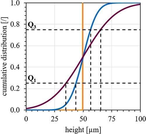
However, it is clear that the deviation of height depends on the size of the scanned area: the larger the area for a given powder, the larger the value obtained will probably be, since the probability of previously described defects occurring in the surface increases, but the percentile is not adjusted. To eliminate this problem as well as to implement a more robust parameter, the difference in quartiles (ΔQ_par) was introduced. To calculate this value, not only two height values but the heights of all found particles are used. If these height values are considered, it can be seen that they follow a certain distribution, as shown as cumulative distributions (S-shaped) for the exemplary surfaces from Figure 11 in Figure 12. For the perfect layer (orange), in which all particles are at the same height, this is a single sharp step. However, the greater the height difference of the particles in the layer, the wider the distribution becomes (blue and purple). From this, it can now be deduced that the width of the distribution directly reflects the roughness of the layer. To describe the width, the interquartile range – a commonly used statistical parameter – was chosen and it was defined as the parameter difference in quartiles. Thus, it applies: the larger the parameter, the higher the interquartile range and thus the wider the distribution. Put simply, the higher the difference in quartiles, the larger the particle height range in which the middle 50% of the particles occur and the rougher the surface.

Figure 12. Cumulative distribution of the height of all found particles referring to the exemplary surfaces illustrated in Figure 11 with the respective marked first (Q₁) and third quartiles (Q₃).

A is the actual surface area, which is calculated by triangulating the surface as shown in Figure 13. For this, both the distance between the pixels in x- and y-direction, which equals the length of a pixel in the corresponding direction (l_{px, x}, l_{px, y}), and the height of the pixels (z) are used (seen in Figure 13 on the left). To calculate the lengths as well as the area of the triangles, the Pythagorean theorem as well as Heron’s formula is used. There is a small difference in the calculated area depending on how it is triangulated (seen in Figure 13 on the right). This difference was therefore evaluated, but it is not significant in the end and can therefore be neglected. Here it applies that the higher the area is, the rougher the surface is.

Figure 13. Detailed triangulation of four pixels (left) and different ways of triangulation (right) [32].

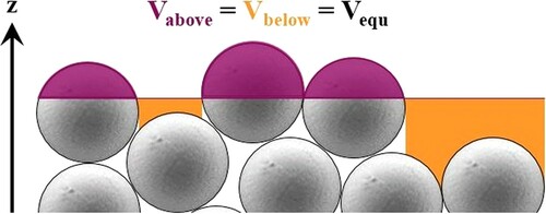
The equalising volume (V_equ) is determined by placing a virtual, perfectly flat plane on the surface. Now the enclosed volume between this plane and the surface, above and below the plane, is calculated. The height of the plane is thereby changed in order to obtain the volume that is identical above and below the plane. This volume is then called the equalising volume. Thus, the enclosed volume above the plane corresponds to the volume of the powder, and the enclosed volume below the plane corresponds to the volume of the cavities. To better visualise the determination of this parameter, it is schematically shown for a two-dimensional surface in Figure 14. In general, the larger the volume, the rougher the surface.

Figure 14. Schematically description of the equalising volume (V_equ).

Finally, the number of particles found in the imaged surface (n_par) itself can be used to describe the roughness of the surface. This parameter provides information about the packing of a spread layer if the particle size remains constant. The following applies: it is assumed that the fewer particles found in the surface, the larger the space between the particles and the rougher the surface, provided powders with the same PSD are compared. However, this parameter is thus also dependent on the size of the imaged area.

2.4. Measuring the powder bed density

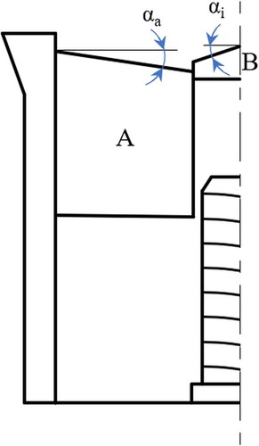
In addition to the test routine for rating the roughness of a spread powder layer, the test routine for measuring the powder bed density – which typically differs from the apparent density measured after [27], as will be shown below – can be integrated into it. To do this, however, the design of the builder must first be considered in a little more detail. Since both the piston (A in Figure 15) and the cap above the spindle, which is intended to protect it from contamination by falling powder (B), were manufactured by turning a Teflon rod, they have a certain conicity and are not ideally flat. For this reason, these two components of the Builder had to be precisely measured with a Mitutoyo Crysta Plus M544 coordinate measuring system. The actual design including inclinations is shown slightly exaggerated in Figure 15. The surface of the piston thus slopes towards the centre with an angle of 0.03939° (=α_a), while the surface of the cover rises towards the centre with an angle of 0.2649° (=α_i), i.e. both are very slightly conical but in opposite directions. The different angles result from the fact that the two components were manufactured at different times and using a different machining setup. This ultimately results in an additional volume, which must be taken into account for an exact determination of the powder bed density.

Figure 15. Cross-section of the builder.

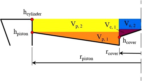
Another additional volume is created by the difference in height between the outer cylinder edge of the builder and its piston as the design used makes it nearly impossible to position the piston at the same level as the outer cylinder edge within a few micrometers. Since the cover over the spindle is merely inserted into its opening and therefore does not represent a fixed connection, its height can also change marginally in the range of a few microns relative to the piston of the builder as a result of cleaning following an experiment, where the cap might be moved slightly during vacuuming the piston. So now, in order to measure the powder bed density as well, the difference in height between the outer edge of the cylinder and the piston of the builder, as well as the cover, must be measured after initialisation. For this purpose, the control software was slightly adapted so that the builder is already initialised when the lifting platform is still in its upper position to simplify the subsequent removal of the builder for measuring. It is then electrically disconnected from the control unit and removed from the Spreading Tester. Using a Mitutoyo ID-C125B dial gauge, the height differences between the points marked in Figure 16 are measured along a total of four measuring sections, each arranged at an angle of 90° to the other. In this figure, the previously described additional volumes (V_p and V_c) are also marked in colour. To calculate these, the respective four height differences are averaged and the areas drawn in the figure are considered as rotationally symmetrical bodies with the corresponding previously determined angles (α_a and α_i). Here, the additional volume created due to the conicity V_{p, 1} is 0.0174 cm³ and V_{c, 1} is 0.0021 cm³, both of which are always constant, and the total additional volume after initialisation (V_p + V_c) determined in this step is about 1.03 cm³ on average.

Figure 16. Enlarged cross-section of the builder with the marked spots for measuring the height differences in red (h_cylinder, h_platform and h_cover) and the marked additional volumes (V_p, and V_c).

After the builder was sized, it is weighed to determine the empty mass of the builder and then placed back into the Spreading Tester. Then the builder is electrically reconnected to the control unit and the test procedure described in Section 2.3 is continued. The only difference is that the builder has already been initialised and this step is therefore omitted. The height of the builder is only set to zero in the control software.

In order for the powder bed density to be calculated correctly, however, there is another additional volume that must be taken into account. This is created by the distance between the cylinder edge of the builder and the blade, which is specified by the setting of the gap size already described in Section 2.3. Thus, the volume of a cylinder with the height of the gap size and the diameter of the piston of the builder has to be added here.

At the end of a spreading test, the lifting platform moves up and the piston of the builder is initialised again. This lowers it to the lowest possible position within the cylinder, which protects the powder bed as best as possible. Now, the outer wall of the builder is carefully tapped with a spatula, causing powder adhering to the inner wall of the cylinder to fall down onto the powder bed below in order not to be vacuumed in the next step. Then, the upper cylinder edge of the builder is carefully vacuumed with an industrial vacuum cleaner to remove excess powder, which would falsify the measuring result. Then the outer wall of the builder is also vacuumed to remove any powder that may have fallen off during removal of the builder and which now adheres to the outside of the builder. Now the builder is weighed and by subtracting the empty mass of the builder, the mass of spread powder contained by the builder is obtained. The height of the piston within the builder is always recorded in a log file and can therefore be easily obtained at the end of the test. Thus, with the help of the inner diameter of the builder, the spread volume can be calculated. Here, the previously described additional volumes must be added, and finally, the powder bed density can be calculated on the basis of the spread powder mass and the total volume in which the powder was spread.

If the measurement of the powder bed density has been integrated into the test routine for evaluating the roughness of a powder layer, this final procedure, starting with the initialisation of the piston within the builder, on which the spread powder bed is present, is carried out after the acquisition of the three-dimensional images for the roughness testing procedure (in order to avoid affecting the surface by tapping). Therefore, the builder is again placed in the Spreading Tester afterwards.

2.5. Evaluating the surface coverage of a single spread powder layer

The Spreading Tester also enables measurement of the surface coverage (ψ) of a single spread powder layer. In this process, the spreading of powder on already melted material from the underlying layer is at least tentatively mimicked and can therefore be investigated. For this purpose, the builder is replaced by a dummy, which is composed of two separate parts, as shown in Figure 17.

Figure 17. Dummy for measuring the surface coverage of a single spread powder layer.

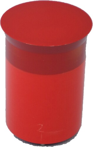
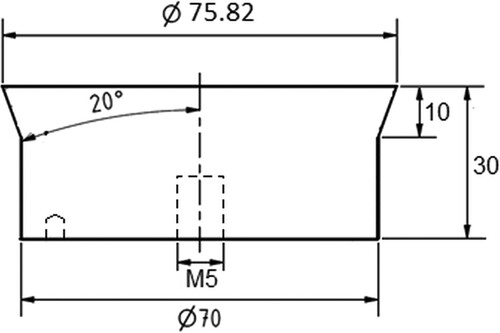
The upper part is a cylinder made of AlMgSi1 turned to fit the recess of the builder in the Spreading Tester. This cylinder has a thread on the underside to connect it to the polymer lower part and a small bore into which a small metal pin from the lower part protrudes, so that the two parts can always be connected to each other in the same orientation. The technical drawing of this component is shown in Figure 18. This cylinder was then refinished by first mirror polishing the top surface and then hard anodising the entire component in red. This produced a slightly roughened but nevertheless flat surface, which is particularly wear-resistant to the spread metal powders and differs strongly in colour from the powder particles. The surface roughness value (R_a) is 0.45 µm. Compared with a surface melted via a LB-PBF AM technique, such as SLM, on which the next powder layer is subsequently spread, this value is about one order of magnitude lower [31], but it is still a good approximation of spreading powder on already melted material from the underlying layer like in the real process. At this point, it should be mentioned that in a first try the red anodised surface was also mirror polished. However, when then trying to spread powder on the mirror-smooth surface, it was found that the particles only came to rest on the surface with difficulty and thus, despite a very high gap size (about three times the d_{50, 3}-value) to allow as many particles as possible to pass through the gap between the dummy and the recoater blade, hardly any covered layers could be spread. It is therefore necessary that a surface, such as that of the building platform or of already melted material from a layer below, has a certain roughness so that the powder can be spread on it.

Figure 18. Technical drawing of the upper part of the dummy.

The lower part of the dummy, on the other hand, is a simple cylinder turned from a red PVC rod, which is firmly connected to the upper part via a bolt. Owing to the lighter material, some weight is saved here, which is necessary to avoid overloading the objective stage of the digital microscope to be used subsequently. On the lower side of the PVC cylinder, analogous to the builder, there are three bolts arranged at an angle of 120° to each other and a rectangular recess was made for the spring contacts through which the builder is normally connected to the control unit. This guarantees that the dummy is always placed in the Spreading Tester in the same way and orientation, which also plays a decisive role for the reproducibility of the tests.

2.5.1. Testing routine for evaluating the surface coverage of a single spread powder layer

To measure the surface coverage of a single spread powder layer, the builder is replaced by the dummy, and this is put in the Spreading Tester on the elevated lifting platform. As with the other test, the Spreading Tester is then connected to the computer using the ‘Direct Mode’ software, which means that all subsequent movements of the Spreading Tester have to be done manually via the software. First, the lifting platform is lowered and the motor of the feeder is initialised. Now, the still loose blade is positioned above the centre of the dummy and the gap size is set analogously to the procedure described for rating the roughness of a spread powder layer in Section 2.3. Then, the powder is poured in the feeder, the blade is initialised backwards to its right position, thereby it wipes off excess powder of the feeder and pulls it in the overflow bin on the right. The blade is then carefully cleaned with a brush, the piston within the feeder is elevated by about 1 mm and the required spreading velocity for the following experiment is set using the software. After that, the blade is moved forward across the dummy to reach the overflow bin on the other side and thereby spreads the single powder layer on the dummy. To prevent the powder from falling down into the electronics and mechanics of the lifting platform, when it is elevated, also in this process the space between the dummy of the builder and the surrounding outer Teflon ring (seen in Figure 1) is cleaned with a fine brush. As the lifting platform is elevated, the dummy is removed from the Spreading Tester and carefully transported to the Keyence VHX-5000 digital microscope next door. The special specimen plate that prevents the builder from rotation so that it can always be placed on the stage in the same orientation also fits for the dummy. As in the method for rating the roughness of a spread powder layer, three-dimensional images of the surface of the single spread powder layer are made, although for the evaluation of the surface coverage only the crisp two-dimensional image is needed. However, the three-dimensional image is still taken in order to obtain the crisp 2D image from the red surface of the dummy away to the top of the highest particle in the powder layer. This time, for imaging a single spread powder layer only four different spots in the size of 7 × 9 single images using the VH-Z100UT objective equipped with a diffuser and 200× magnification are stitched. Thereby, the four spots are always at the same position arranged centred on the dummy. With the used settings the depicted area of a single stitched image here is in the size of approximately 8.25 × 8.25 mm.

2.5.2. Analysing algorithm for evaluating the surface coverage of a single spread powder layer

After the image acquisition process, the crisp two-dimensional images are now analysed once more by a self-written algorithm using Python 3.5 and a free module called OpenCV. It primarily has the task of distinguishing between the particles and the red underground which simulates the already melted material of the underlying layer in a real building process.

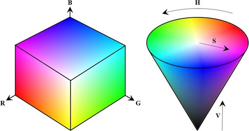
First, the images are opened by the written algorithm in a classic RGB colour space. However, in order to be able to process the images with the desired module, they have to be converted into the so-called HSV colour space. While the RGB colour space (Red, Green and Blue) is structured like a cube, the HSV colour space (Hue, Saturation and Value) is structured like a cone. For better understanding, both colour spaces are shown in Figure 19.

Figure 19. Cube-shaped RGB colour space (left) and cone-shaped HSV colour space (right).

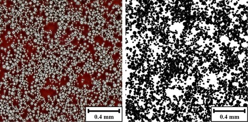
After the image has been successfully converted, preselected segments of the HSV colour space are selected piece by piece and marked, which means that those corresponding pixels are stored in a masking matrix that belongs to the preselected red colour range. The HSV colour segments to be marked were determined in advance with several images, whereby the HSV values of all pixels were listed for each image and those that could be assigned to the red area of the dummy were filtered out as best as possible. This resulted in numerous contiguous HSV colour segments, which are then used to mark the corresponding pixels. Since these are very numerous, they are not specifically mentioned in the following. Once all areas of the image have been marked according to the preselected segments, the masking matrix is used to create a simple black and white image. This step can be seen in a full-size image in Figure 20 and in a magnified area of the image in Figure 21. Finally, the algorithm determines the fraction of black pixels that can be assigned to the particles and thus corresponds to the surface coverage. The shown example has a size of 8.1 × 8.0 mm, comes from an experiment of plasma spheroidised powder with 60 µm gap size, 50 mm s⁻¹ spreading velocity using the HSS blade and shows a surface coverage of 56.5%.

Figure 20. Crisp two-dimensional image (left) and masked B/W image (right).

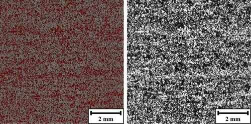
Figure 21. Crisp two-dimensional image of a magnified area from Figure 20 (left) and the corresponding masked B/W image (right).

2.6. Tests performed and evaluation of the reproducibility

Using the plasma spheroidised IN718 powder, the reproducibility of all described test methods was investigated. For this purpose, each test was conducted a total of five times. Thus, the results of these tests only represent a sample of the population. The following characteristic values calculated from this sample therefore refer to it. The true mean (µ) of a population would be calculated from an infinite number of repeated measurements using Equation (1). If there is no systematic error in the measurements, this is also the true value of the quantity to be measured. Now, since the number of measurements (n) is a finite number, in contrast to Equation (1), the calculated mean value is only an approximation of the true value.

Equation (1): Calculation of the true mean (µ) of a population using the value of a single measurement (x_i) and the total number of measurements (n) $\mu =\underset{n\to \mathrm{\infty }}{lim}{\displaystyle \frac{{\sum }_{i=1}^n{x}_i}{n}}$

As described, a defined number of spots (n) for the method of rating the roughness (n = 9) and for the method of evaluating the surface coverage (n = 4) in the spread powder surface are examined for each single measurement. Using the single measurement values of the spots (x_{spot, i}), an arithmetic mean value (x_i) and the corresponding standard deviation for this sample (s_i) are calculated as shown in Equation (2).

Equation (2): Calculation of the standard deviation of a sample (s_i) using the single measurement values of the spots (x_{spot, i}) $s_i=\sqrt{{\displaystyle \frac{{\sum }_{i=1}^n{\left(x_{spot,i}\right)}^2-{\displaystyle \frac{{\left({\sum }_{i=1}^n{x}_{spot,i}\right)}^2}{n}}}{n-1}}}$

If the standard deviations of the arithmetic means of the five individual measurements differ from each other, they are afflicted with different uncertainties. Therefore, a weighted mean value $\left(\overline{\mathrm{x}}\right)$ is calculated as shown in Equation (3), using the arithmetic mean value (x_i) and the corresponding standard deviation (s_i) of all single measurements. Thus, a value with a lower uncertainty is now weighted more heavily.

Equation (3): Calculation of the weighted mean value $\left(\overline{\mathrm{x}}\right)$ using the arithmetic mean value (x_i) and standard deviation (s_i) of all single measurements $\overline{\mathrm{x}}={\displaystyle \frac{{\sum }_{i=1}^n{\displaystyle \frac{x_i}{s_i^2}}}{{\sum }_{i=1}^n{\displaystyle \frac{1}{s_i^2}}}}$

In order to be able to express the reproducibility in a number, the standard deviation of the weighted mean value $\left(\overline{\mathrm{s}}\right)$ is first calculated. It must be considered that the arithmetic mean values of the individual measurements (x_i) are needed for this (see Equation (3)), which also already have a certain standard deviation (s_i). Therefore, the Gaussian error propagation law (see Equation (4)) has to be used for the calculation.

Equation (4): Calculation of the standard deviation of the weighed mean value $\left(\overline{\mathrm{s}}\right)$ considering the Gaussian error propagation law $\overline{\mathrm{s}}=\sqrt{{{\sum }_{i=1}^n{\displaystyle \frac{\mathrm{\partial }f\left(x_i\right)}{\mathrm{\partial }{x}_i}\cdot s_i}}^2}$In this case, the function f(x_i) is equal to the formula for calculating the weighted mean value $\left(\overline{\mathrm{x}}\right)$ from Equation (3). Consequently, if the partial derivation is performed, the term given in Equation (5) is obtained for the standard deviation sought.

Equation (5): Derived form of the formula for calculating the standard deviation $\left(\overline{\mathrm{s}}\right)$ considering the Gaussian error propagation law $\overline{\mathrm{s}}=\sqrt{{\sum }_{k=1}^n{\displaystyle \frac{s_k^2}{{\sum }_{i=1}^n{\left({\displaystyle \frac{s_k}{s_i}}\right)}^2}}}$

If the resulting standard deviation of the weighted mean value is then related to the weighted mean value, the relative standard deviation (RSD) is obtained, which in this case represents the reproducibility of the methods for rating the roughness and evaluating the surface coverage. The calculation of the relative standard deviation is given in Equation (6).

Equation (6): Calculation of the relative standard deviation (RSD) representing the reproducibility $\mathrm{R}\mathrm{S}\mathrm{D}={\displaystyle \frac{\overline{\mathrm{s}}}{\overline{\mathrm{x}}}\cdot 100\text{\%}}$

The reproducibility for the powder bed density measurement method, on the other hand, is quite simple to determine because only one value is obtained from a single measurement. Therefore, it is not necessary to calculate a weighted mean value and its standard deviation considering the Gaussian error propagation law, but a simple arithmetic mean value and its standard deviation can be calculated according to Equation (2). The standard deviation is then related to the arithmetic mean value analogously to Equation (6), which finally represents the reproducibility for the powder bed density measurement method.

For investigating the reproducibility of the test method for rating the roughness of the top spread powder layer, the EOS-inspired spreading routine was chosen. Further, the Spreading Tester was equipped with the rhombic HSS blade, the gap size as well as the layer thickness was set to 40 µm, the spreading velocity was set to 150 mm s⁻¹ and the total number of spread powder layers was set to 50.

For investigating the reproducibility of the test method to determine the powder bed density, again the EOS-inspired spreading routine was chosen, and the rhombic HSS blade was mounted. The gap size as well as the layer thickness was set to 50 µm, the spreading velocity was set to 150 mm s⁻¹ and the total number of spread powder layers was set to 50. To additionally demonstrate the influence of the different spreading routines, the powder bed density was determined with the Concept Laser-inspired spreading routine and otherwise identical settings. Here, however, it should be stated that this test was then only carried out twice.

The reproducibility of the test method for examining the surface coverage of a single spread powder layer could only be investigated using the EOS-inspired spreading routine, since the dummy used cannot be moved in order to mimic the spreading routine inspired by a Concept Laser machine. However, once more the HSS blade was used, the gap size was set to 50 µm and the spreading velocity was set to 150 mm s⁻¹.

3. Experimental results and discussion

3.1. Basic characteristics of the powder

In Figure 22 an SEM image of the plasma spheroidised IN718 powder is shown. Evidently, the particle shape is almost perfectly spherical. Only just a few smaller satellites attached to the bigger particles can be seen. This is also confirmed by the very high sphericity value of the powder measured by dynamic image analysis (CAMSIZER). The volume-related sphericity value is listed together with the volume-related characteristic d-values in Table 1. Owing to this spherical shape, the measured powder characteristics, as listed in Table 2, are well suited for powders used in AM. The flow time is very low, and the apparent density is not much lower than the tap density, which both are very high as well. The tap density determines the maximum achievable density of the loose powder heap. A densification beyond this is only possible by applying pressure, for example, by a punch.

Figure 22. SEM image of the plasma spheroidised IN718 powder used.

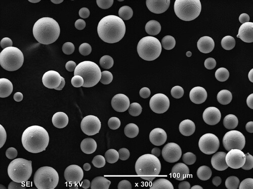
Table 1. Volume-related characteristic d-values (d_{10, 3}, d_{50, 3}, d_{90, 3}) and volume-related sphericity (SPHT3).

d10, 3 [µm]	d50, 3 [µm]	d90, 3 [µm]	SPHT3 [/]
22.9	33.3	44.6	0.967

Table 2. Basic powder characteristics (FR = flow rate; ADH = apparent density measured using a Hall funnel; ADA = apparent density measured using an Arnold Meter; TD = tap density) of the plasma spheroidised IN718 powder used.

FT [s/50 g]	ADH [g cm^−³]	ADA[g cm^−³]	TD [g cm^−³]
10.1 ± 0.1	4.67 ± 0.02	4.83 ± 0.01	4.96 ± 0.01

3.2. Evaluating the reproducibility

In Table 3 the surface roughness-related evaluated values (ΔH_par, ΔQ_par, V_equ, A, n_par) are given. Each arithmetic mean value (x_i) and its corresponding standard deviation (s_i) of a single measurement, is an average of the values for the nine spots examined on the spread powder layer. Furthermore, the calculated weighted mean value $\left(\overline{\mathrm{x}}\right)$ and its standard deviation $\left(\overline{\mathrm{s}}\right)$ as well as the relative standard deviation (RSD), of all parameters are listed. It can be seen from this that generally good relative standard deviations for all parameters in a range of 0.91–4.81% were achieved, representing the reproducibility of the measurement. This means that the Spreading Tester yields well reproducible surface roughness-related values. In general, the lowest value for the relative standard deviation, i.e. the best reproducibility, was observed for the parameter surface area (A) and then, in increasing order, for the equalising volume (V_equ), number of particles found (n_par), difference in quartiles (ΔQ_par) and deviation of height (ΔH_par).

Table 3. Surface roughness-related (ΔH_par, ΔQ_par, V_equ, A, n_par) arithmetic mean values (x_i) including their standard deviation (s_i) of the five single measurements and the weighted mean value $\left(\overline{x}\right)$, its standard deviation $\left(\overline{s}\right)$ and relative standard deviation (RSD) calculated from this.

	ΔHpar [µm]	ΔQpar [µm]	Vequ [mm³]	A [mm²]	npar [/]
x1 ± s1	74.5 ± 5.1	19.9 ± 0.5	(1.74 ± 0.03) E-02	4.76 ± 0.04	937 ± 13
x2 ± s2	77.9 ± 2.8	21.0 ± 1.1	(1.82 ± 0.03) E-02	4.87 ± 0.05	934 ± 26
x3 ± s3	75.1 ± 4.0	20.1 ± 1.3	(1.75 ± 0.02) E-02	4.75 ± 0.05	966 ± 29
x4 ± s4	77.3 ± 6.7	20.1 ± 1.2	(1.77 ± 0.03) E-02	4.78 ± 0.06	946 ± 15
x5 ± s5	66.7 ± 2.5	18.0 ± 0.9	(1.58 ± 0.04) E-02	4.55 ± 0.04	983 ± 29
$\overline{\mathrm{x}}$	72.8	19.7	1.74E-02	4.72	945
$\overline{\mathrm{s}}$	3.5	0.8	2.98E-04	0.04	19
RSD [%]	4.81	3.97	1.71	0.91	1.99

For the single spread layers, the arithmetic mean values (x_i) including their standard deviation (s_i) of the evaluated surface coverage (ψ) of the five single measurements and the calculated weighted mean value $\left(\overline{\mathrm{x}}\right)$ as well as its standard deviation $\left(\overline{\mathrm{s}}\right)$ and the relative standard deviation (RSD) are listed in Table 4. Again, with a value of 3.98% for the relative standard deviation it can be stated that the reproducibility of this test method is fine.

Table 4. Arithmetic mean values (x_i) including their standard deviation (s_i) of the surface coverage (ψ) of the five single measurements and the weighted mean value $\left(\overline{x}\right)$, its standard deviation $\left(\overline{s}\right)$ and relative standard deviation (RSD) calculated from this.

	Ψ [%]
x1 ± s1	35.4 ± 0.9
x2 ± s2	34.6 ± 1.6
x3 ± s3	35.8 ± 1.7
x4 ± s4	33.8 ± 2.3
x5 ± s5	33.9 ± 1.8
$\overline{\mathrm{x}}$	35.0
$\overline{\mathrm{s}}$	1.4
RSD [%]	3.98

As the powder bed density (ρ_pb) is measured just once per experiment, no standard deviations of the single measurements are given. Thus, only the values of the five single measurements (x_i), their arithmetic mean value (x_ave) and its standard deviation (s_i) as well as the relative standard deviation (RSD) are listed in Table 5. With a value of 0.24% for the relative standard deviation, this test method is the most reproducible among the developed methods.

Table 5. Powder bed density (ρ_pb) of the five single measurements (x_i), arithmetic mean value (x_ave), its standard deviation (s_i) and relative standard deviation (RSD).

	ρpb [g cm^−³]
x1	4.81
x2	4.80
x3	4.80
x4	4.82
x5	4.83
xave	4.81
si	0.01
si – %	0.24

3.3. Influence of the spreading strategy on the powder bed density

As mentioned above, the influence of the spreading strategy, which describes the individual process steps during spreading, should be illustrated with a rather small-scale experiment. This was already investigated in [12], but since the method for determining the powder bed density has been modified and thus has become more accurate since then, as well as to give just one example of what the Spreading Tester is capable to do, this experiment was repeated for the present study.

In Table 6 all measured filling characteristics are listed, whereby the measurement of the apparent densities (ADH, ADA) and the tap density (TD) was repeated three times, whereas the measurement of the powder bed densities (ρ_{pb, EOS}, ρ_{pb, CL}) was repeated only twice. It shows that the powder bed density using the Concept Laser-inspired spreading strategy is higher than that using the EOS-inspired spreading strategy. This can be attributed to the additional process step of wiping off excess powder when using the Concept Laser-inspired spreading strategy as during the backward movement of the blade, the powder bed is thereby slightly compacted with the sloping side of the blade.

Table 6. Measured filling characteristics of the plasma spheroidised IN718 powder used listed in increasing order: ADH = apparent density measured using a Hall funnel; ρ_{pb, EOS} = powder bed density measured using an EOS-inspired spreading strategy; ADA = apparent density measured using an Arnold Meter; ρ_{pb, CL} = powder bed density measured using a Concept Laser-inspired spreading strategy; TD = tap density.

ADH [g cm^−³]	ρpb, EOS [g cm^−³]	ADA [g cm^−³]	ρpb, CL [g cm^−³]	TD [g cm^−³]
4.67 ± 0.02	4.81 ± 0.01	4.83 ± 0.01	4.87 ± 0.00	4.96 ± 0.01

Furthermore, it can be seen that the measured powder bed density of the plasma spheroidised powder used is only slightly below the tap density and very similar to the apparent density measured by the Arnold Meter. Thus, the Arnold Meter method is apparently more suitable for describing the filling properties of particularly spherical powders used for powder bed-based AM techniques than the funnel method (Hall or Carney funnel) since it mimics the procedure better. However, further tests would be necessary to generalise this statement. In any case, it is clear that the classical funnel method for measuring the apparent density [27] is not applicable for AM.

4. Conclusions

In this study, a new testing device, the so-called Spreading Tester, was introduced as well as a total of three different methods to test powders used for LB-PBF AM techniques. This offers the possibility to further enlighten the process of spreading powder layers in powder bed-based additive manufacturing and collect more data for these powders, which is still lacking at the moment. The reproducibility of the newly developed testing methods was investigated using a plasma spheroidised and therefore highly spherical powder. Furthermore, a small-scale experiment was carried out, just to give an example of what can be done using the Spreading Tester. The results can be summarised as follows:

1. By using the Spreading Tester, the LB-PBF process is mimicked accurately. The relevant process parameters such as layer thickness, gap size, spreading velocity, spreading strategy and many others can be set freely within wide margins and can thus be adapted to the upcoming build job the powder should be tested for. It is therefore a powerful tool to investigate powders used in LB-PBF AM techniques.

2. The first test method is used to rate the surface roughness of the top spread powder layer. It therefore provides information about the quality of a spread powder layer on a loose powder bed.

3. The second test method is used to determine the powder bed density. It describes the filling behaviour of a loose powder bed for powders used in LB-PBF AM techniques. It can also be integrated into the testing procedure of the first test method.

4. The third and last test method is used to evaluate the surface coverage of a single spread powder layer, which is quite similar to spreading on already selectively melted material from the layer below during the real AM process. Thus, this test provides information on how a powder behaves when it is not spread on a loose powder bed but on the already melted material, which is also part of the manufacturing process and makes a big difference.

5. All test methods combined therefore shed light on many aspects of the LB-PBF process. They can be used to compare the ability of similar powders to be spread, also called spreadability, in LB-PBF AM techniques. The reproducibility of the test methods was very satisfactory, even though this is a first attempt and the Spreading Tester is still a prototype and therefore there is certainly still room for optimisation.

6. It could be shown that for highly spherical powders, the apparent density measured using an Arnold Meter is fairly similar to the powder bed density measured by the Spreading Tester. On the other hand, the apparent density measured using a funnel is not well suited to describe the filling behaviour of highly spherical powders used in LB-PBF AM techniques since it does not imitate the process accurately enough.

7. In the small-scale experiment it could be shown that using the Concept Laser-inspired spreading strategy results in a higher powder bed density compared to using the EOS-inspired spreading strategy. This is due to the additional process step of wiping off excess powder from the powder bed with the sloping side of the blade before selective melting is done.

Disclosure statement

No potential conflict of interest was reported by the author(s).

Additional information

Notes on contributors

Marco Mitterlehner

Marco Mitterlehner studied Technical Chemistry at the Technische Universität Wien, Austria, where he also did his PhD thesis. He started working in the field of Additive Manufacturing during his master studies in 2015. Throughout his university research, Mr. Mitterlehner was particularly concerned with the spreadability, storage and processing of AM powders. He is now working as process and product developer for AM powders in the R&D department of voestalpine Böhler Edelstahl GmbH & Co KG in Kapfenberg, Austria.

Herbert Danninger

Herbert Danninger is retired professor for Chemical Technology of Inorganic Materials at Technische Universität Wien, Vienna, Austria. He has been active in powder metallurgy for more than 40 years and is author/co-author of 500+ publications. From 2009 to 2020 he was chairman of the ‘Gemeinschaftsausschuss Pulvermetallurgie', the PM association of the German-speaking countries. He holds honorary doctoral degrees of Technical University Cluj-Napoca (Romania), Universidad Carlos III de Madrid (Spain) and Universitatea din Craiova (Romania) and is Fellow of APMI and EPMA. In 2020 he was awarded the ‘Ivor Jenkins Medal’ of IOM3.

Christian Gierl–Mayer

Christian Gierl-Mayer studied Technical Chemistry at Technische Universität Wien (TU Wien), Vienna, Austria. He got his Master in 1996 and his PhD in 2000 from TU Wien. After 3 years in private research institute (ofi-Austrian Research Institute of Chemistry and Technology) he re-joined the powder metallurgy group of Prof. Herbert Danninger as senior researcher. He got his habilitation in 2019 for ‘Thermoananlytical Investigation of Interactions between Powder Metallurgy Steels and the Atmosphere during Sintering’, and became Associate Professor in 2019. He is currently leading the research group Powder Metallurgy at TU Wien and the Division Chemical Technologies, Institute of Chemical Technologies and Analytics. His publication record is about 260 publications in journals and conference proceedings, 4 book chapters and 7 patents.

Johannes Frank

Since 1999 Johannes Frank is employed at the Technische Universität Wien (TU Wien), Vienna, Austria. He started as technician at the Institute of Materials Chemistry. In 2013 he became leader of the Joint Workshop of the Faculty of Technical Chemistry at the TU Wien. He is responsible for design, construction and fabrication of prototypes and machinery.

Wolfgang Tomischko

Wolfgang Tomischko has worked in the electronics industry since leaving school in 1977. He has worked in this field as a developer in several Austrian medium-sized companies. Since 2007 he has been a technical employee at the Technische Universität Wien, Vienna, Austria. Since 2014, he has also held a lectureship in the field of electrical engineering at the same university.

Harald Gschiel

Harald Gschiel has studied Technical Chemistry at the Vienna University of Technology, where he also did his PhD thesis focusing on Powder Metallurgy and Solid Oxide Fuel Cells. After leaving university in 2015, he has been constantly working in the field of Additive Manufacturing, now employed at voestalpine Böhler Edelstahl GmbH & Co KG. His topics are mainly powder processing, powder characterization and product development.

References

- Parteli EJR, Pöschel T. Particle-based simulation of powder application in additive manufacturing. Powder Technol. 2016;288:96–102.
- Haeri S. Optimisation of blade type spreaders for powder bed preparation in additive manufacturing using DEM simulations. Powder Technol. 2017;321:94–104.
- Jacob G, Brown CU, Donmez A. The influence of spreading metal powders with different particle size distributions on the powder bed density in laser-based powder bed fusion processes. US Department of Commerce. National Institute of Standards and Technology. 2018.
- Mitterlehner M, Danninger H, Gierl-Mayer C. Study on the layer building of powders in powder bed fusion processes for additive manufacturing. In: Proceedings of the Euro PM2018 Congress & Exhibition; 2018 Oct 14–18; Bilbao, Spain. Shrewsbury (United Kingdom): European Powder Metallurgy Association (EPMA); 2018. ID 3988826.
- Mitterlehner M, Danninger H, Gierl-Mayer C. A new method for describing the morphology of powder layers in direct laser melting. In: Proceedings of the 3rd Metal Additive Manufacturing Conference 2018; 2018 Nov 21–23; Vienna, Austria. Leoben (Austria): Austrian Society for Metallurgy and Materials (ASMET); 2018. p. 31–40.
- Nan W, Pasha M, Bonakdar T, et al. Jamming during particle spreading in additive manufacturing. Powder Technol. 2018;338:253–262.
- Alchikh-Sulaiman B, Carriere PR, Chu X, et al. Powder spreading and tribocharging for additive manufacturing process. In: Proceedings of the Euro PM2019 Congress & Exhibition; 2019 Oct 13–16; Maastricht (Netherlands). Shrewsbury (United Kingdom): European Powder Metallurgy Association (EPMA); 2019. ID 4347446.
- Gopaluni A, Lyckfeldt O, Hatami S. Powder Spreadability in metal additive manufacturing. Paper presented at: Alloys for Additive Manufacturing Symposium 2019; 2019 Sep 18–20; Göteborg, Sweden.
- Schrage J, Schleifenbaum JH. Influence of powder application parameters on powder bed properties and on productivity of laser powder bed fusion (L-PBF). In: Proceedings of the 4th Metal Additive Manufacturing Conference 2019; 2019 Sep 30-Oct 2; Örebro (Sweden). Leoben (Austria): Austrian Society for Metallurgy and Materials (ASMET); 2019. p. 28–37.
- Cordova L, Bor T, Md S, et al. Measuring the spreadability of pre-treated and moisturized powders for laser powder bed fusion. Addit Manuf. 2020;32:101082. doi:10.1016/j.addma.2020.101082.
- Mitterlehner M, Danninger H, Gierl-Mayer C, et al. Study on the influence of the blade on powder layers built in powder bed fusion processes for additive manufacturing. BHM, Berg- Huettenmaenn Monatsh. 2020;165(3):157–163.
- Mitterlehner M, Danninger H, Gierl-Mayer C, et al. Spreading behaviour and packing density of the powder bed in L-PBF as a function of spreading strategy and velocity. In: Proceedings of the Euro PM2020 Virtual Congress & Exhibition; 2020 Oct 5–7. Shrewsbury (United Kingdom): European Powder Metallurgy Association (EPMA). ID 4854670.
- Lorenzo M, Hulme-Smith C. Flowability of steel and tool steel powders: a comparison between testing methods. Powder Technol. 2021;384:402–413.
- Hulme-Smith C, Hari V, Mellin P. Spreadability testing of powder for additive manufacturing. BHM, Berg- Huettenmaenn Monatsh. 2021;166(1):9–13.
- Mitterlehner M, Danninger H, Gierl-Mayer C, et al. Investigation of the influence of powder moisture on the spreadability using the spreading tester. BHM, Berg- Huettenmaenn Monatsh 2021;166(1):14–22.
- Shaheen MY, Thornton AR, Luding S, et al. The influence of material and process parameters on powder spreading in additive manufacturing. Powder Technol. 2021;383:564–583.
- Si L, Zhang T, Zhou M, et al. Numerical simulation of the flow behavior and powder spreading mechanism in powder bed-based additive manufacturing. Powder Technol. 2021;394:1004–1016.
- Wang L, Zhou Z, Li E, et al. Powder deposition mechanism during powder spreading with different spreader geometries in powder bed fusion additive manufacturing. Powder Technol. 2022;395:802–810.
- Zhang J, Tan Y, Xiao X, et al. Comparison of roller-spreading and blade-spreading processes in powder-bed additive manufacturing by DEM simulations. Particuology. 2022;66:48–58.
- Prescott JK, Barnum RA. On powder flowability. Pharm Technol. 2000;24:60–84.
- Vock S, Klöden B, Kirchner A, et al. Powders for powder bed fusion: a review. Prog Addit Manuf. 2019;4(4):383–397.
- Hare C, Zafar U, Ghadiri M, et al. Analysis of the dynamics of the FT4 powder rheometer. Powder Technol. 2015;285:123–127.
- Lumay G, Boschini F, Traina K, et al. Measuring the flowing properties of powders and grains. Powder Technol. 2012;224:19–27.
- Powder Rheology [Internet]. Graz (AT): Anton Paar GmbH. c2021. [cited 2021 Jul 4]; Available from: https://wiki.anton-paar.com/en/powder-rheology/
- Ensuring High Quality in the Additive Manufacturing Process [Internet]. Haan (GE): Microtrac Retsch GmbH. c2020 [cited 2020 Jul 1]. Available from: https://www.microtrac.de/dltmp/www/5e396c14-fe94-4af0-83c0-7f30c3c9c754-49caf39811f8/tr_additive_manufacturing_vs_0519_en.pdf
- International Organization for Standardization (ISO). Metallic powders – determination of flow rate by means of a calibrated funnel (Hall flowmeter). Vernier: ISO; 2018. Standard No. 4490:2018.
- International Organization for Standardization (ISO). Metallic powders – determination of apparent density – Part 1: Funnel Method. Vernier: ISO; 2018. Standard No. 3923-1:2018.
- American Society for Testing and Materials International (ASTM International). Standard test method for apparent density of metal powders and related compounds using the Arnold Meter. West Conshohocken: ASTM. Standard No. B703 - 17
- International Organization for Standardization (ISO). Metallic powders – determination of tap density. Vernier: ISO; 2011. Standard No. 3953:2011.
- Mitterlehner M, Danninger H, Gierl-Mayer C. Study on segregation effects in powder layers built in powder bed fusion processes for additive manufacturing. In: Proceedings of the Euro PM2019 Congress & Exhibition; 2019 Oct 13–16; Maastricht (Netherlands). Shrewsbury (United Kingdom): European Powder Metallurgy Association (EPMA); 2019. ID 4346412.
- Mitterlehner M, Danninger H, Gierl-Mayer C, et al. Processability of moist superalloy powder by SLM. BHM, Berg- Huettenmaenn Monatsh. 2021;166(1):23–32.
- Mitterlehner M. Metal powders for laser powder bed fusion technologies: storing, drying, spreading, printing [PhD thesis]. Vienna (AT): Technische Universität Wien; 2020.