Comparison of methods for characterising the steel cleanness in powder metallurgical high-speed steels

ABSTRACT

Powder metallurgical (PM) steels are characterised by a very high cleanness level. Single mesoscopic inclusions can nevertheless induce material failure under the extreme exposed stresses in the final product. Extensive knowledge about the cleanness of these steels is therefore essential. Various methods for inclusion analyses are available, providing different information about the non-metallic inclusion population present in the steel matrix. Several state-of-the-art methods of inclusion analysis are compared, considering morphological parameters and chemical composition of the detected inclusions as well as the required time effort and statistics behind the specific method. Tests were carried out with a standard PM steel HS6-5-3C. Combined with chemical extraction, automated SEM/EDS measurements enable a clear description of the microscopic cleanness level. Statistical analyses using the extreme value theory allowed the prediction of the maximum inclusion size in the investigated samples.

KEYWORDS:

• Powder metallurgy
• high-speed steel
• non-metallic inclusion
• cleanness

1. Introduction

Steel cleanness is becoming an increasingly important quality feature due to the ever-increasing demands on materials. As a result of this development, various processes have been established in the production of special steels which enable a significant improvement in steel cleanness [1]. Past research shows that steel cleanness can be significantly improved by vacuum treatments such as vacuum induction melting (VIM) [2]. Various works have also shown that subsequent remelting treatments such as vacuum arc remelting (VAR) cause a significant reduction in the overall inclusion population compared to the initial state [3]. The powder metallurgical (PM) production of steels can also be mentioned here as a process that, according to the current state of research, also leads to excellent results with regard to steel cleanness [4].

Tool steels produced by powder metallurgy (PM) are increasingly crucial in processing other materials. Due to their higher wear resistance and ductility, PM steels are often superior to conventional materials in machining and forming. The property profiles of PM steels can be attributed to the production process, which involves atomisation of the steel melt and subsequent hot isostatic pressing of the produced powder [5]. Previous research has shown that due to the rapid solidification of the molten steel during atomisation, no extensive carbide networks are formed. Despite the high carbon content, spherical carbides are evenly distributed throughout the material [6]. The advantages of gas atomisation with subsequent HIP treatment compared to water atomisation and sintering, which primarily results in higher density and thus higher strength of the materials produced, have already been described in detail in previous research [7]. Considering the fine carbide distribution, the presence of non-metallic inclusions (NMIs) is of essential importance for the final product quality [4]. This is particularly the case for highly specialised applications such as bearings for aircraft engines or tools for highly abrasive materials, which place high demands on the respective steels [8]. Steel cleanness is already very high in these steels, and the overall inclusion number is marginal compared to classical production of these high-alloyed steels. Nevertheless, non-metallic inclusions in the meso- and macroscopic size range are occasionally observed. Inclusions larger than 20 µm in diameter are statistically difficult to find due to their small number and the usually limited analysed sample area or volume. However, these inclusions are the most harmful regarding material defects [9].

Various methods have been developed to determine the different properties of inclusions in the steel. Despite the constant improvement in the field of inclusion analysis, no single approach has yet been developed that can analyse the inclusion landscape in its entirety. Light optical microscopy, for example, is a standardised method currently used for the specific investigation of inclusion size and distribution [10]. Another technique, examination by SEM/EDS, has been established to examine inclusions of sizes below the analytical limits of other methods [11–13]; this has been documented as a remarkably versatile method, especially in combination with preparation steps such as chemical or electrolytic extraction. [14] The relevance of selecting an appropriate method has been highlighted in various publications listing and comparing current methods for inclusion analysis [15,16]. Each method offers certain advantages and disadvantages, an assessment of which is to be made in this work specifically for PM steels. However, it is relevant to consider the broadest-possible overview since various research has shown that different inclusion properties influence the decisive properties of the related materials. For example, studies have shown a relationship between the size and shape of inclusions and the fatigue properties of the materials concerned [17]. Furthermore, specific inclusion properties can impact the steel-production processes, as with clogging during continuous casting [18]. As a result, inclusion analysis research is increasingly focused on highly specialised materials with high demands for certain properties [19].

In the present work, various methods of inclusion analysis are compared in terms of possible information on size distributions in different size ranges, chemical composition, number and morphology, especially considering the described challenges in PM tool steels. Cleanness is studied in a high-speed steel HS6-5-3C, applying different methods for microscopic cleanness evaluations as well as high cycle and ultra-high cycle fatigue tests to find larger inclusions. A statistical analysis based on the extreme value theory also predicts the maximum inclusion size in the examined steel.

2. Materials and methods

The investigated material was melted on laboratory scale in a vacuum induction furnace with a chemical composition according to HS6-5-3C high-speed steel grade and atomised with nitrogen gas. In order to maintain a sufficiently high degree of non-metallic inclusions, no special measures were taken to produce a very clean material during melting operations. The obtained powder was filled in capsules, evacuated, densified by hot isostatic pressing (HIP) and subjected to a forging process as well as a soft-annealing treatment. The steel composition, with the DIN/EN designation HS6-5-3C, is given in Table 1. All samples for the described subsequent analyses were cut from one bar material of the defined steel grade.

Table 1. Chemical composition of the examined steel.

C [wt%]	Si [wt%]	Mn [wt%]	Cr [wt%]	Mo [wt%]	V [wt%]	W [wt%]	S [wt%]	O [wt%]
1.29	0.60	0.30	4.20	5.00	3.00	6.30	0.012	0.004

2.1. Cycle fatigue tests

High cycle fatigue (HCF) and very high cycle fatigue (VHCF) tests were carried out to investigate the NMIs which initiate the fracture. The test parameters and further specifications of the tests are given in Table 2.

Table 2. Specifications of the CF tests.

Parameter	HCF-test	VHCF-test
Test temperature	∼23°C	∼23°C
Stress ratio	0.1	−1
Test frequency	∼158 Hz	∼965 Hz
Stress amplitude	700 MPa	820–960 MPa
Mean stress	856 MPa	0
Test arrangement	Tension arrangement	Tension compression arrangement

Both series of tests were carried out with an axial application of the stress. A Rumul Testronic 100 resonance testing machine was used for the HCF tests and an IMV i210 electrodynamic shaker for the VHCF tests.

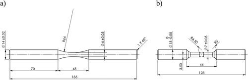
The specimens for both types of tests were made from slices cut from the HIP capsules in the cross direction of the forging. The sample geometries used in the HCF and VHCF tests are shown in Figure 1. The fractured surface was also investigated using the SEM. In order to be able to minimise the influence of surface roughness, the samples were polished in the notched area to a mean roughness value Ra of 0.2.

Figure 1. Sample geometries used in the HCF (a) and VHCF (b) tests.

After hardening at 1070°C for 20 minutes, a tempering treatment with three tempering steps of two hours each at approx. 560°C was applied to a target hardness of the material of 62 HRC, which corresponds to the application hardness.

In order to determine the effect of the inclusion size on the fatigue endurance strength in the HCF regime, the threshold stress intensity factor ΔK_th was calculated for each HFC test. The threshold stress intensity factor ΔK_th, which refers to internal inclusions, is calculated from the amplitude stress σ_a and the square root of the area of the inclusions found on the fracture surface (fracture trigger) √area [20]: (1) $\mathrm{\Delta }{K}_{th}=0.5\times {\sigma }_a\sqrt{\pi \sqrt{\mathrm{area}}}$(1)

It should be noted that the described connection between defect size and fatigue endurance strength does not take into account the hardness of the material and so the calculated value for the threshold stress intensity factor ΔK_th only applies to a specific hardness (62 HRC).

2.2. Light optical microscopy

A light optical microscope (Olympus MX61A) was used to analyse the defined steel's inclusion features on 16 metallographic specimens. The minimum detectable inclusion size was 10 µm. The average size of the region of interest was 400 mm². The size and area of the detected inclusions and the distance to their nearest neighbours were recorded. Corrections to the data following the automated examination with the microscope software were made to eliminate false inclusion findings (e.g. scratches or impurities).

2.3. Chemical extraction

A 5% nital solution was used as the solvent for the chemical extraction. The samples were exposed to the solvent in a beaker for a time dependent on the particular experiment. The specifications of the tests and the sample shapes used are summarised in Table 3.

Table 3. Parameters for extraction experiments.

Specimen	Solvent	Sample shape (W x D x H)	Duration	Filter
E1	5% nital solution (sequential)	Approx. 1 × 1 × 1 cm	2 hours (15-minute sequences)	1 µm + 10 µm
E2	5% nital solution	Approx. 1 × 1 × 1 cm	5 days	1 µm + 10 µm
E3	5% nital solution	Approx. 1.5 × 1.5 × 2 cm	7 days	1 µm + 10 µm
E4	5% nital solution + 30% HCL	Approx. 1 × 1 × 1 cm	2 hr + 5 sec	1 µm + 10 µm

The solvent-precipitate mixture was then emptied from the beaker and separated from one another in a vacuum filter device using a membrane filter (see Table 3). In the sequential extraction, the aim was to achieve a time-limited contact between the NMIs and the solvent by siphoning off the sediment produced by the dissolution at particular time intervals using a pipette and transferring it to the filter device [21]. After these steps, the sample and the filter were examined using a scanning electron microscope with energy dispersive spectroscopy (SEM/EDS) to characterise the shape, composition and number of inclusions.

2.4. Manual and automated SEM/EDS measurements

Samples were cut from the material and mounted onto a conductive resin. They were ground and subsequently polished to a mirror finish. A JEOL 7200F SEM was used for manual and automated investigations. The parameter settings for the automated SEM/EDS measurements on the JEOL SEM are summarised in Table 4.

Table 4. Parameters for automated SEM/EDS measurements.

SEM/EDS process parameters	Numerical value
Acceleration voltage [kV]	15
Electric charge [pC]	14
Dead time [%]	34
Number of counts input [cps]	120,000
Number of counts output [cps]	78,000
Resolution [pxl]	1024
Pixel/feature [pxl]	9
Magnification [-]	130 (3-µm feature)/400 (1-µm feature)
Measurement time [s]	1
Gray value limit [-]	15,000
Gray value matrix [-]	20,000

After the automated measurements, an acceleration voltage of 20 kV was used for the elemental mappings.

Since the entire steel sample can only be analysed with considerable time and effort when measuring NMI using SEM/EDS, statistical methods are used in order to be able to draw conclusions about the entirety from those measurements.

Extreme value theory is a branch of statistics that deals with the evaluation and prediction of rare events (extreme cases). Within these methods, statistical values such as the probability of the occurrence of an extreme case are inferred on the basis of samples. In relation to the statistical analysis of NMIs, the size of the largest possible inclusion in a steel sample can be estimated [22].

The generalised Pareto distribution (GPD) method is based on a family of standardised distributions that result from the measured values exceeding limit values. The value of the exceedances of the limit values can be calculated for a variety of output distributions of the measured values, by means of the function (2) $F(x)=1-{\left(1+{\displaystyle \frac{\xi (x-u)}{{\sigma }^{\mathrm{\prime }}}}\right)}^{-1/\xi }$(2)

which, in addition to the size of the inclusion x, also contains the boundary value u and the size and shape parameters σ′ and ξ [23].

The GPD method was applied to the SEM data to predict the maximum inclusion size in a given volume V. To calculate the size of the largest inclusion x_max, the occurrence probability of the largest possible inclusion F(x_max) is related to the expected number of inclusions larger than the limit value N_V(x > u) [24]: (3) $N_V(x>u)V(1-F(x_{\max }))=1$(3)

By substituting the general equation for the log-normal distribution as seen in Equation (2), into Equation (3), Equation(4) is derived: (4) $x_{\max }=u-{\displaystyle \frac{{\sigma }^{\mathrm{\prime }}}{\xi }(1-{(N_V(x>u)V)}^{\xi })}$(4)

This formula, in addition to the size of the inclusion x, also contains the boundary value u and the size and shape parameters σ′ and ξ, respectively [23].

The actual number higher than the limit value N_V(x > u) of the inclusion can be deduced from the size of this circular area and the calculated cutting probabilities; in the present case, the Woodhead method was applied [25].

For this purpose, the inclusions found are divided into different groups based on their size. The number of inclusions in a group is distorted by the intersection of a plane, so inclusions can appear smaller than they actually are. This is remedied by subtracting from the number of inclusions in a group those inclusions that have been incorrectly classified. These misclassifications can be calculated by summing the product of inclusion number in a group and the corresponding cut probability parameter for those groups that are smaller than the group under consideration. Dividing the difference between the two values by the probability of correct classification gives the actual number of inclusions in a group [25].

To determine the size and shape parameters σ′ and ξ, both constants can be derived from a mean excess (ME) plot based on the SEM feature measurements. A regression line is placed over the linear range in the ME diagram; the parameters can now be determined from the slope k and the intersection d, using the following Equations (5) and (6): (5) $k={\displaystyle \frac{\xi }{1-{\xi }^{\mathrm{\prime }}}}$(5) (6) $d={\displaystyle \frac{{\sigma }^{\mathrm{\prime }}}{1-{\xi }^{\mathrm{\prime }}}}$(6) The determination of the parameters ξ, σ′ and N_V(x > u) makes it possible to calculate the maximum inclusion size in any sample volume by inserting them into Equation (4) [26].

Another way of calculating the size of the largest inclusion is the method known as the Gumbel or Weibull distribution. This method is also based on the data from automated SEM/EDS measurements. The largest inclusion is determined from each recorded segment of the analysis and the inclusions obtained are ranked according to size. The size of the selected inclusions x is then plotted against the parameter Y calculated from the sequence number i and the total number N. The parameter Y is calculated as follows [27]: (7) $Y=-\mathrm{Ln}\left(-\mathrm{Ln}\left({\displaystyle \frac{i}{N+1}}\right)\right)$(7)

The slope k and the vertical intercept d can then be determined from the diagram created and an inserted regression line. These are related to the shape parameters of the Gumbel distribution in the following way [27]: (8) $k={\displaystyle \frac{1}{\delta }}$(8) (9) $d=-{\displaystyle \frac{\lambda }{\delta }}$(9)

An estimate of the largest existing inclusion x_max in an examined volume V_i can then be given from the determined values. The following relationship applies [28]: (10) $x_{\max }=\lambda +\delta \times Y_i$(10)

Where Y_i establishes a relationship between the reference volume V₀ and the observed volume V_i [28]: (11) $Y_i=-\mathrm{Ln}\left(-\mathrm{Ln}\left(1-{\displaystyle \frac{V_0}{V_i}}\right)\right)$(11)

3. Results

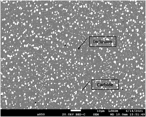
A specific microstructure is formed due to the unique cooling conditions in powder-metallurgical production. The characteristic microstructure is illustrated in Figure 2.

Figure 2. Carbide and inclusion distribution of the investigated material HS6-5-3C in a SEM image captured using a backscattered electron detector.

3.1. Cycle fatigue behaviour

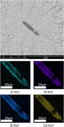
In all of the methods performed, the largest inclusions were detected on the surfaces of samples tested using HCF. This is consistent with results from previous research showing that the cycle fatigue test can be used as a way to find the most damaging inclusions in a volume [29]. These inclusions, which act as fracture triggers, are approx. 50–150 µm in size and located in the CaO-SiO₂-Al₂O₃ system. One example of a detected inclusion is shown together with its chemical mapping in Figure 3.

Figure 3. SEM-image in BSE-mode of a fracture-initiating inclusion on the fracture surface of a HCF specimen with corresponding EDS-elemental mappings.

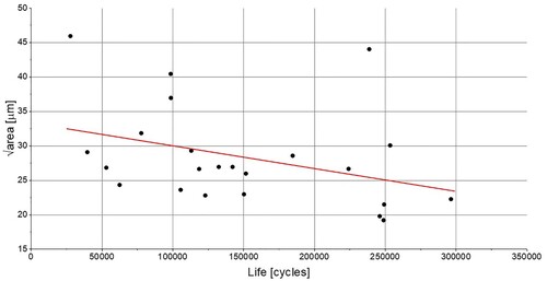
An evaluation of the relationship between the inclusion size and the load changes sustained by the samples was carried out in the HCF tests. For this purpose, the size parameter was plotted against the load cycles in Figure 4 and a regression line based on the data was inserted.

Figure 4. Relationship between the inclusion size and the load changes sustained by the samples in the HCF tests.

In contrast to the HCF tests, no inclusions were found on the fracture surface in the VHCF tests. A closer examination showed that the fracture in these samples originated from the surface.

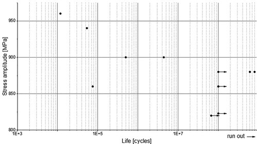
Another difference in the comparison HCF test is that the stress amplitude was varied in the VHCF test. In Figure 5, the respective applied stress amplitudes of the tests are plotted against the number of load cycles until the samples break. It should be noted that four of the samples tested were discontinued prior to actual fracture.

Figure 5. Applied stress amplitudes of the tests are plotted against the number of load cycles.

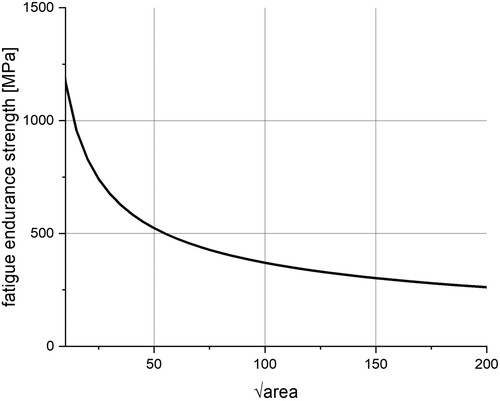
The threshold stress intensity factor ΔK_th for the respective HCF tests was calculated from the relationship shown in Equation (1) and a mean value was calculated. The relationship between the fatigue endurance strength and the inclusion size shown in Figure 6 can be established from the mean value, which assumes a value of 3.3 MPam^1/2 for the examined material. In Figure 6 only the influence of inclusions is shown.

Figure 6. Relationship between the fatigue endurance strength and the inclusion size.

3.2. Light optical microscopy

In order to show the inclusion distribution of the 16 samples analysed, the results of each sample were presented in a boxplot (see Figure 7); this shows that the light microscopy method had a lower limit of 10 µm for the size of detectable inclusions. Furthermore, it shows that the mean inclusion sizes for the samples were between 12 µm (Sample 11) and 26 µm (Sample 3). The largest inclusion found in all of the specimens had a size of 57 µm (Sample 3).

Figure 7. Box plot of sample inclusions found using light optical microscopy.

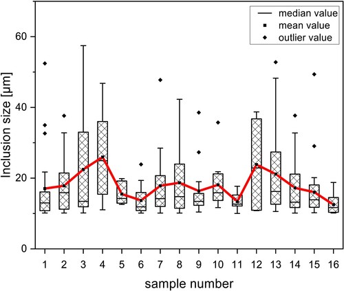
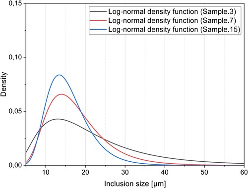
To compare the inclusion size distributions of different samples, which show apparent differences in Figure 7, the density functions of the inclusion sizes of three specimens were plotted (see Figure 8). The selected samples showed distinct differences in size distributions, although derived from the same bar material.

Figure 8. Log-normal distribution function of three selected specimens.

3.3. Chemical extraction

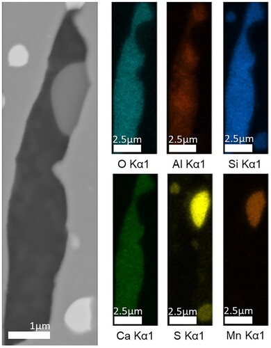
Even with a 7-day duration using a 5% nital solution as the solvent, inclusions could still be found. As exemplarily demonstrated in Figure 9, oxides remain stable over a long time.

Figure 9. SEM-image in BSE-mode of oxide inclusions found on the filter after chemical extraction of specimen E3 (Duration: 7 days) with corresponding EDS-elemental mappings.

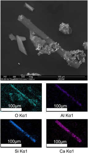
After the sequential extraction, using 5% nital solution, oxide inclusions were also found on the 1-µm filter. Here, significantly more inclusions were found when analysing the filter cake, than with any other extraction method. Figure 10 shows an example of extracted inclusions, ranging in size from 1 µm to >100 µm.

Figure 10. SEM-image in BSE-mode of oxide inclusions found on the filter after chemical extraction of specimen E1 (duration: 2 hours in 15-minute sequences) with corresponding EDS-elemental mappings.

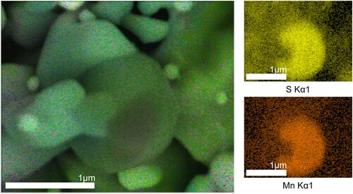
The extraction of samples using longer solvent exposure times resulted in the dissolution of all sulphide inclusions. Only with sequential extraction sulphides could be found in the filtrate; an example of these is exemplarily shown in Figure 11.

Figure 11. SEM/EDS elemental mapping of sulphide inclusions found on the filter after chemical extraction of specimen E1 (duration: 2 hours in 15-minute sequences).

3.4. SEM/EDS results

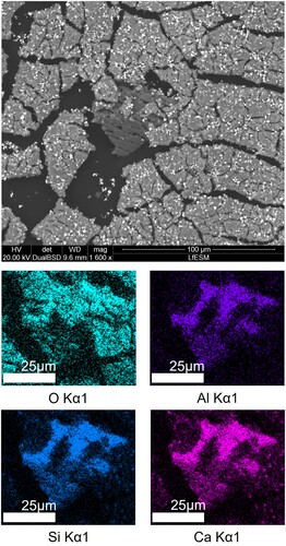
Inclusions of various types were identified on sample sections using SEM mappings. These inclusions comprised oxide–sulphides, sulphides and oxides (in order of prevalence), with a size range of 1–20 µm. One example, an oxide–sulphide inclusion, is shown in Figure 12.

Figure 12. SEM-image in BSE-mode of oxide-sulphide inclusions found on specimen 7 with corresponding EDS-elemental mappings.

During the automated SEM/EDS measurement of the bar material, no inclusions with a size larger than 30 µm were detected on the examined cross-section. Figure 13 illustrates the composition distribution of the micro-cleanness, composed of oxide–sulphides, sulphides, oxides and nitride sulphides (in order of prevalence). The average ECD measured on specimen 7 was 1.3 µm.

Figure 13. Composition distribution of the micro-cleanness (specimen 7).

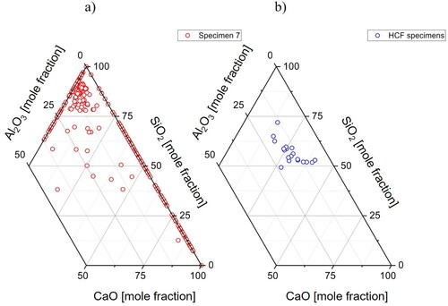
A comparison of the chemical compositions of the inclusions found on the fracture surfaces of the HCF and the automated SEM/EDS measurements of specimen 7 was performed (see Figure 14). Compared to the Al₂O₃-containing oxides in specimen 7, the HCF oxides exhibited a similar aluminium and a higher calcium content.

Figure 14. Comparison of inclusion composition between specimen 7 (a) and HCF samples (b) analysed with automated SEM/EDS.

A statistical analysis based on the data of automated SEM/EDS measurements was conducted to generate further information. The largest possible inclusions (for oxide–sulphides, sulphides and oxides) in the given sample volume were calculated using the GPD method. For calculations within the framework of the GPD method, the SEM/EDS data must correspond to a log-normal distribution [30]. To ensure this pre-condition, the Anderson–Darling tests for log-normal distribution were performed in Minitab [31]. The GPD procedure was applied to all examined data sets by creating ME plots as the first step of the analysis using the software R. Figure 15 shows an example of a ME plot considering the specimen 7 oxide data.

Figure 15. ME plot of specimen 7 oxide data.

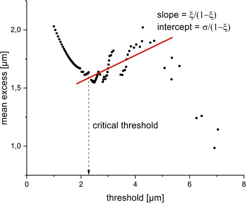
The shape parameters of the function can be determined from the ME plot. To calculate the size of the largest possible inclusion, the number of inclusions in relation to the investigated volume must be determined and entered into Equation (2) along with the shape parameters of the log-normal distribution. As previously described, the function of the size of the largest possible inclusion, which depends on the sample volume, can be determined in Equation (2). In Table 5, all determined parameters are summarised.

Table 5. Determined parameters of the investigated specimens.

Specimen	Type of inclusion	Shape parameters σ′	Shape parameters ζ	Inclusion density [1/mm^3]
3	Sulphides	0.114	0.121	82,986
7	Sulphides	0.143	0.044	156,295
15	Sulphides	0.108	0.102	166,813
3	Oxide–sulphides	0.199	0.097	115,117
7	Oxide–sulphides	0.482	0.035	124,730
15	Oxide–sulphides	0.175	0.123	116,348
3	Oxides	0.556	0.228	2316
7	Oxides	0.894	0.313	8738
15	Oxides	0.797	0.203	2675

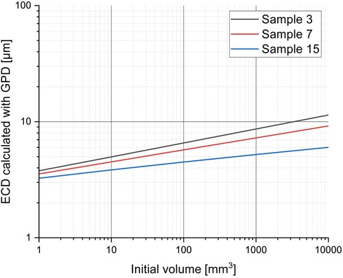
Through inputting the parameters shown in Table 5 into Equation (2), graphs were plotted to estimate the sizes of the largest inclusions in a given volume. As an example, Figure 16 shows the generated plot for the sulphide data.

Figure 16. Estimations of the largest sulphide inclusion in a given volume.

The same SEM/EDS data sets used for the GPD method were also used to apply the Gumbel distribution. For this purpose, the largest oxide–sulphides, sulphides and oxides of the recorded segments were ranked in the manner described in Section 2.4 and plotted in an ECD vs. Y diagram. The shape parameters δ and λ can be calculated from the inserted regression lines of the respective curves using Equations (8) and (9). The maximum inclusion size can then be estimated using Equation (10). The results for the Gumbel distribution in direct comparison to the calculated maximum inclusion sizes of the GPD method for the individual inclusion groups (the average values of all three samples) are summarized in Table 6 together with the calculated reference volume of the individual samples. Based on the HCF sample geometry, both methods assume an examined volume of approx. 7000 mm².

Table 6. Calculated maximum inclusion sizes of the GPD method compared with the results for the Gumbel distribution.

Inclusion group	Results GPD	Results Gumbel distribution
Oxide–sulphides	Approx. 15 µm (ECD)	Approx. 6 µm (ECD)
Sulphides	Approx. 10 µm (ECD)	Approx. 3 µm (ECD)
Oxides	Approx. 150 µm (ECD)	Approx. 13 µm (ECD)

4. Discussion

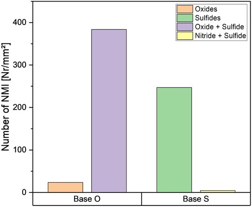
By summarising the findings of the applied methods, a comparison of the analytical limitations of the methods is made possible (see Table 7). The inclusions were categorised into oxides, sulphides and oxide–sulphides to enable the comparability of test results and calculated values of the GPD method.

Table 7. Method matrix with the findings from the performed analyses.

Method	Detected size	Results GPD	Detectable morphology	Detectable distribution	Detectable composition
SEM/EDS	10–100 µm	Sulphide approx. 10 µm (ECD) Oxide–sulphide approx. 15 µm (ECD) Oxide approx. 150 µm (ECD)	Yes (2D)	Yes	Yes
Manual SEM/EDS in combination with HCF	50–150 µm		Yes (3D)	No	Yes
Manual SEM/EDS in combination with extraction	10–150 µm		Yes (3D)	No	Yes
Automated SEM/EDS measurements	>1 µm		Yes (2D)	Yes	Yes
Light optical microscopy	10–50 µm		Yes (2D)	Yes	No

Figure 11 shows that the sulphide particles have a globular shape, similar to the oxide–sulphides. As shown in Table 7, the sulphides and oxide–sulphides have ECDs of 10 and 15 µm, respectively, calculated using the GPD method. This agrees with the diameters of globular sulphides and oxide–sulphides observed using the SEM.

Due to the forming after processing, the oxidic inclusions show clear elongations, as seen in Figure 3. If the ECD value (shown in Table 7) calculated using the GPD method were to be converted into the maximum length of an elongated inclusion, the size would be substantially higher than the largest inclusions found (approx. 150 µm). This can be explained by the fact that the GPD method assumes globular inclusions, particularly in the Woodhead analysis. Therefore, in contrast to those of sulphide and oxide–sulphide inclusions, the calculated maximum inclusion sizes for oxide inclusions are not in accordance with the observed values. This demonstrates that GPD is unsuitable for estimating the sizes of elongated inclusions.

In contrast to the GPD method, the calculated maximum inclusion sizes for all inclusion types in the Gumbel distribution are significantly smaller than reality reflects. Even if it is known from the literature that the Gumbel distribution in conventional steels is a reliable method for estimating the maximum inclusion size, this is not the case based on the results for the steel examined in the present study. The reason for the higher accuracy of the GPD method when it comes to at least oxide–sulphides and sulphides can be explained by the fact that statistically it is an extreme value theory method which can better deal with rare, large inclusions in steels with high steel cleanness, while the Gumbel distribution is only based on the evaluation of a distribution. Nevertheless, further investigations should carried out on this aspect in the future.

The largest inclusions were detected on the fracture surface of the HCF samples (100–150 µm); however, cyclic fatigue testing is not recommended as a future standard method for cleanness analysis due to its time-consuming nature and high costs. However, this method's high inclusion-size detection limit presents a target to be achieved with other more-efficient methods. Light optical microscopy could not detect inclusions with a size of more than 100 µm, as it was limited to a single sample cross-section each. The probability of finding a macroscopic inclusion on an inspected cross-section is low due to their rarity. Even across 16 samples, the analysed area was too small and no macroscopic inclusions were detected (see Figure 7). This method is further limited by its inability to generate information on the composition or 3D morphology of inclusions. In summary, light optical microscopy does not offer the possibility to consistently find macroscopic inclusions without considerable additional effort.

The evaluation of the tested material with regard to the fatigue properties shows that the fatigue endurance strength is influenced by internal inclusions in a similar way to conventional steels. The value for the threshold stress intensity factor ΔK_th of these steels, at 3.3 MPam^1/2, is in a similar range to that of other steels known from the literature [20]. Since other factors influencing fatigue strength, such as the basic hardness of the material and the carbide size, play a subordinate role, this illustrates the relevance of inclusions in those steels that act as critical defects.

In most methods, the SEM/EDS analysis was conducted in combination with different preparation steps. This was done to compensate for the disadvantages associated with SEM/EDS measurements, such as difficulties in finding rare, especially large inclusions on a single cross-section and in the analysis of the 3D morphology of inclusions. An advantage of chemical extraction is that the detected inclusions can also be analysed with regard to their 3D morphology. A comparison of all extraction attempts shows that sequential extraction with nital solution is the most suitable method to expose inclusions in the investigated steel. This method increases the detectability of large oxidic inclusions (see Figures 9 and 10). Although sulphide inclusions are not the main objective of this work, this type can also be exposed through sequential extraction and subsequently analysed (see Figure 11), which is advantageous for better understanding the overall inclusion scenario. The associated additional effort for extractions is negligible in these circumstances. Overall, it can be concluded that processing by sequential extraction, with nital solution, is a suitable method to obtain more information from the investigated high-alloyed samples. The automated SEM/EDS analysis provided useful information about the examined steel. The chemical composition of the micro-inclusions, as shown in Figure 13, includes relevant information about steel cleanness in general. Furthermore, combined with the GPD method, it also allows for estimating the largest inclusion in a sample.

During the detailed examination of the bar material by the described methods, it was possible to collect a large amount of information about the inclusions. Throughout the investigations, the most frequent inclusions of the oxide-sulphides were determined to be manganese oxide-sulphides. At the same time, sulphides were particularly manganese sulphides and oxides were predominantly particles located in the CaO-SiO₂-Al₂O₃ system. In addition, the morphology of the different inclusion types could also be examined in detail.

All tested methods, on their own, only provided part of the information about the inclusion landscape present in the steel. None of the tested methods offers all the following benefits: analysis of size distribution across a wide range, determination of the composition, detection of the largest inclusion and consideration of the inclusion morphology. The current work suggests that combining several methods is a suitable solution. Based on all of the tests, it has become clear that this combination should initially consist of examining a sample using automated SEM/EDS measurements. This data provides information about micro- and meso-cleanness (composition, size distribution, etc.) and a starting point for statistical investigations. This, particularly the GPD method, should be used after further studies to determine the maximum inclusion size and, thus, cover the macro-cleanness within the size distribution. Following the SEM/EDS investigations, a sequential extraction with a nital solution as a solvent should be conducted. This approach is particularly suitable with a view to further research.

5. Conclusion

Detailed analysis of non-metallic inclusions is becoming increasingly important to improve the properties of modern PM steels continuously. In the past, this has led to research focused on new and very specialised methods to study steel cleanness. This work aimed to select the best-suited approach to gain a possibly comprehensive overview of non-metallic inclusions in PM high-speed steel. In particular, the central challenge is the possibility of finding meso- and macroscopic but rare inclusions. Based on the literature review, several potential methods were selected and compared. A set of methods was subsequently used for a practical series of tests. The main finding of this work can be summarised as follows:

• Despite the many available methods for cleanness assessment, no method can provide all the information needed. For this reason, a combination of methods was selected, enabling a possibly comprehensive overview on the inclusions present in the steel matrix. Combining automated SEM/EDS measurements, sequential extraction and statistical analyses based on the field of extreme value theory showed the most promising results.

• Results of the GPD method showed a satisfying correlation to measured inclusion sizes for sulphides and Oxide–sulphides. Due to the non-globular appearance of oxides in the analysed samples, disparities are observed for this inclusion type.

• A clear correlation between microscopic cleanness and the larger inclusions detected in the HCF test was observed, especially regarding their chemical composition. So far, only formed bar material has been investigated.

• The influence of inclusions on the fatigue endurance strength of powder metallurgical steels with high hardness and small carbide size was investigated.

This combination of different methods produces a wide range of relevant information, which will support future research in the field of steel cleanness, with a particular focus on powder metallurgical steels. Further analyses considering samples during the PM production process itself might be helpful to study inclusion evolution over the process in more detail and can provide non-deformed oxides for statistical considerations.

Disclosure statement

No potential conflict of interest was reported by the author(s).

Additional information

Funding

The financial support by the Austrian Federal Ministry of Labour and Economy, the Austrian National Foundation for Research, Technology and Development (Österreichische Nationalstiftung für Forschung, Technologie und Entwicklung) and the Christian Doppler Research Association is gratefully acknowledged.

Notes on contributors

M. Schickbichler

Manuel Schickbichler is a PhD student at the Christian Doppler Laboratory for Inclusion Metallurgy in Advanced Steelmaking.

S. Ramesh Babu

Shashank Ramesh Babu is a postdoc at the Christian Doppler Laboratory for Inclusion Metallurgy in Advanced Steelmaking.

M. Hafok

Martin Hafok is an employee at voestalpine Böhler Edelstahl GmbH & Co KG, working in the Research and Development department.

C. Turk

Christoph Turk is an employee at voestalpine Böhler Edelstahl GmbH & Co KG, working in the Research and Development department and is head of the product and process development area.

G. Schneeberger

Gerald Schneeberger is an employee at voestalpine Böhler Edelstahl GmbH & Co KG, working in the powder metallurgy plant and being an assistant manager there.

A. Fölzer

Andreas Fölzer is an employee at voestalpine Böhler Edelstahl GmbH & Co KG, working in the powder metallurgy plant and manager there.

S. K. Michelic

Susanne Michelic is a professor at the Chair of Ferrous Metallurgy at the Montanuniversitaet Leoben and head of the Christian Doppler Laboratory for Inclusion Metallurgy in Advanced Steelmaking.

References

- Zhang L, Thomas BG. State of the art in evaluation and control of steel cleanliness. ISIJ Int. 2003;43(3):271–291. doi:10.2355/isijinternational.43.271.
- Feng H, Li H-B, Liu Z-Z, et al. Cleanliness control of high nitrogen stainless bearing steel by vacuum carbon deoxidation in a PVIM furnace. Metall and Materi Trans B. 2021;52(6):3777–3787. doi:10.1007/s11663-021-02291-7.
- Yang S, Yang S, Qu J, et al. Inclusions in wrought superalloys: a review. J Iron Steel Res Int. 2021;28(8):921–937. doi:10.1007/s42243-021-00617-y.
- Fölzer A, Tornberg C. Advances in processing technology for powder-metallurgical tool steels and high speed steels giving excellent cleanliness and homogeneity. MSF. 2003;426–432:4167–4172. doi:10.4028/www.scientific.net/MSF.426-432.4167.
- Tornberg C, Fölzer A. New optimised manufacturing route for PM tool steels and High Speed Steels. 6th International Tooling Conference: The Use of Tool Steels; 2002 Sept; Karlstadt, Sweden.
- Tornberg C, Fölzer A. Less carbide means fewer cracks in tools made from gas-atomised steel. Met Powder Rep. 2005;60(6):36–40. doi:10.1016/S0026-0657(05)70434-3.
- Zhang Y, Feng E, Mo W, et al. On the microstructures and fatigue behaviors of 316L stainless steel metal injection molded with gas- and water-atomized powders. Metals. 2018;8(11):893. doi:10.3390/met8110893.
- Iqbal A, King J. The role of primary carbides in fatigue crack propagation in aeroengine bearing steels. Int J Fatigue. 1990;12(4):234–244. doi:10.1016/0142-1123(90)90450-S.
- Sohar CR, Betzwar-Kotas A, Gierl C, et al. PM tool steels push the edge in fatigue tests. Met Powder Rep. 2009;64(2):12–17. doi:10.1016/S0026-0657(09)70013-X.
- Bytyqi A, Pukšič N, Jenko M, et al. Characterization of the inclusions in spring steel using light microscopy and scanning electron microscopy. Mater Technol. 2011;45(1):55–59.
- Bandi B, Santillana B, Tiekink W, et al. 2D automated SEM and 3D X-ray computed tomography study on inclusion analysis of steels. Ironmak Steelmak. 2020;47(1):47–50. doi:10.1080/03019233.2019.1652437.
- Capurro C, Boeri R, Cicutti C. Characterization of nonmetallic inclusions of Al-killed Ca-treated steels by automated SEM/EDS and its application to industrial case studies. Steel Research Int. 2022: 2200152. doi:10.1002/srin.202200152.
- Nuspl M, Wegscheider W, Angeli J, et al. Qualitative and quantitative determination of micro-inclusions by automated SEM/EDX analysis. Anal Bioanal Chem. 2004;379(4):640–645. doi:10.1007/s00216-004-2528-y.
- Ramesh Babu S, Michelic SK. Analysis of non-metallic inclusions by means of chemical and electrolytic extraction – a review. Materials (Basel, Switzerland). 2022;15:9. doi:10.3390/ma15093367.
- Doostmohammadi H, Karasev A, Jönsson PG. A comparison of a two-dimensional and a three-dimensional method for inclusion determinations in tool steel. Steel Research Int. 2010;81(5):398–406. doi:10.1002/srin.200900149.
- Wang Y, Karasev A, Jönsson PG. Comparison of nonmetallic inclusion characteristics in metal samples using 2D and 3D methods. Steel Res Int. 2020;91(7):1900669. doi:10.1002/srin.201900669.
- Zerbst U, Madia M, Klinger C, et al. Defects as a root cause of fatigue failure of metallic components. II: non-metallic inclusions. Eng Fail Anal. 2019;98:228–239. doi:10.1016/j.engfailanal.2019.01.054.
- Li W, Wang Y, Wang W, et al. Dependence of the clogging possibility of the submerged entry nozzle during steel continuous casting process on the liquid fraction of non-metallic inclusions in the molten Al-killed Ca-treated steel. Metals (Basel). 2020;10(9):1205. doi:10.3390/met10091205.
- Park JH, Kang Y. Inclusions in stainless steels − a review. Steel Res Int. 2017;88(12):1700130. doi:10.1002/srin.201700130.
- Zhang JW, Lu LT, Wu PB, et al. Inclusion size evaluation and fatigue strength analysis of 35CrMo alloy railway axle steel. Mater Sci Eng A. 2013;562:211–217. doi:10.1016/j.msea.2012.11.035.
- Schickbichler M. Extraktion Sulfidischer Einschlüsse aus der Stahlmatrix [bachelor’s thesis]. Leoben, Austria; 2020.
- Beretta S. More than 25 years of extreme value statistics for defects: fundamentals, historical developments, recent applications. Int J Fatigue. 2021;151:106407. doi:10.1016/j.ijfatigue.2021.106407.
- Anderson C, Shi G, Atkinson H, et al. The precision of methods using the statistics of extremes for the estimation of the maximum size of inclusions in clean steels. Acta Mater. 2000;48(17):4235–4246. doi:10.1016/S1359-6454(00)00281-0.
- Anderson CW. The largest inclusions in a Piece of Steel. Extremes. 2002;5(3):237–252. doi:10.1023/A:1024025027522.
- Swinden JWDJ. Kinetics of the nucleation and growth of proeutectoid ferrite in some Fe-C-Cr alloys. J Iron Steel Inst. 1971;209(11):883–899.
- Shi G, Atkinson HV, Sellars CM, et al. Application of the generalized Pareto distribution to the estimation of the size of the maximum inclusion in clean steels. Acta Mater. 1999;47(5):1455–1468. doi:10.1016/S1359-6454(99)00034-8.
- Machado PVS, Araújo LC, Soares MV, et al. The use of a modified critical plane model to assess multiaxial fatigue of steels with nonmetallic inclusions. MATEC Web Conf. 2019;300:16005. doi:10.1051/matecconf/201930016005.
- Ahmad A, Purbolaksono J, Yahya Z. Estimating inclusion size in WE43-T6 magnesium alloys based on Gumbel extreme values. Mater Sci Eng A. 2009;513–514:319–324. doi:10.1016/j.msea.2009.02.030.
- Furuya Y, Matsuoka S, Abe T. A novel inclusion inspection method employing 20 kHz fatigue testing. Metall Mat Trans A. 2003;34(11):2517–2526. doi:10.1007/s11661-003-0011-6.
- Atkinson HV, Shi G. Characterization of inclusions in clean steels: a review including the statistics of extremes methods. Prog Mater Sci. 2003;48(5):457–520. doi:10.1016/S0079-6425(02)00014-2.
- Bag A, Delbergue D, Bocher P, et al. Statistical analysis of high cycle fatigue life and inclusion size distribution in shot peened 300M steel. Int J Fatigue. 2019;118:126–138. doi:10.1016/j.ijfatigue.2018.08.009.