Generating Small Areal Synthetic Microdata from Public Aggregated Data Using an Optimization Method

Abstract

Small area microdata contain attributes and locations of individual members of a population in small census geographies. This type of data is critical in research and policymaking, but it is often not publicly available due to confidentiality concerns. The limited access to small area microdata can result in insufficient data for certain research (data scarcity). Even for researchers qualified to access the small area microdata, their research can hardly be reproduced by others (method irreproducibility). To address these issues, we develop a method to generate small area synthetic microdata (SASM) that is suitable for public use. Specifically, an optimization approach is proposed to minimize the difference between published census tables and the SASM. Two counties in Ohio are used as case studies to test the efficacy of the proposed method and the validity of the resulting SASM. The results show that the SASM aligns not only with the census tables, but also with an external data source that contains a sample of the small area microdata. We also illustrate how the SASM can be used to address data scarcity and method irreproducibility in demographic research.

小区域微观数据包含小普查区的个人属性和位置, 在研究和决策中至关重要, 但由于保密性的考虑而常常无法对外公开。小区域微观数据的限制, 导致研究数据的缺乏(数据稀缺性)。即使研究人员能够获取小区域微观数据, 其研究也很难被复制(方法不可复制性)。为了解决这些问题, 我们开发了适用于公众的小区域合成微观数据(SASM)的制作方法。我们提出的优化方法, 能最大限度地降低公开人口普查表与SASM的差异。通过对美国俄亥俄州两个县的分析, 测试了方法的有效性并验证了SASM。结果表明, SASM不仅与人口普查表一致, 而且与包含小区域微观数据样本的外部数据源一致。我们还阐释了如何用SASM去解决人口研究中的数据稀缺性和方法不可复制性的问题。

Los microdatos de áreas pequeñas contienen atributos y localizaciones de miembros individuales de una población en las pequeñas geografías censales. Este tipo de datos es crucial en investigación y en la formulación de políticas, aunque con frecuencia no están públicamente disponibles por razones de confidencialidad. El acceso limitado a los microdatos de áreas pequeñas puede resultar en insuficiencia de datos para cierto tipo de investigaciones (escasez de datos). Incluso para los investigadores calificados para acceder a los microdatos de áreas pequeñas, su investigación difícilmente puede ser reproducida por otros (irreproducibilidad del método). Para enfrentar estos problemas, desarrollamos un método con el cual generar microdatos sintéticos para áreas pequeñas (SASM), que es adecuado para uso público. Específicamente, se propone un enfoque de optimización para minimizar la diferencia entre las tablas censales publicadas y el SASM. Se usaron dos condados de Ohio como estudios de caso para poner a prueba la eficacia del método propuesto y la validez de los resultados del SASM. Los resultados muestran que el SASM se alinea no solo con las tablas censales, sino también con una fuente de datos externa que contiene una muestra de los microdatos de áreas pequeñas. Ilustramos también el modo como el SASM puede usarse para enfrentar el problema de escasez de datos y la irreproducibilidad del método en investigación demográfica.

Key Words:

• census data
• open and reproducible research
• spatial microdata
• spatial open data
• synthetic population

关键词：:

• 人口普查数据
• 开放式可复制研究
• 空间微观数据
• 开放式空间数据
• 合成人口。

Palabras clave::

• datos abiertos espaciales
• datos censales
• investigación abierta y reproducible
• microdatos espaciales
• población sintética.

Small area microdata consist of a detailed list of individuals from a population, including attributes and location information at a small area level (e.g., the census block level; Tranmer et al. 2005). This type of data provides an individual-level profile of the population, which enables the modeling of individual behavior and interactions and is essential for research and policymaking in fields such as demography, health, and transportation (Ferguson et al. 2005; Gonzalez, Hidalgo, and Barabasi 2008; Ruggles 2014; Ruggles et al. 2015; Alessandretti 2022). Access to small area microdata is often restricted, however, due to privacy laws and regulations. In the United States, for example, the complete record of individual-level census responses is an important source of small area microdata, but these data can be easily linked to publicly available auxiliary data to reveal individuals’ identities (Slavkovic, Kinney, and Karr 2011; Lin and Xiao 2023), and making it public violates Title 13 of the U.S. Code (13 U.S.C. §9). The small area microdata instead are only available to researchers at secure Federal Statistical Research Data Centers (FSRDC). The only public microdata from the Census Bureau are the sample microdata known as the American Community Survey Public Use Microdata Sample (ACS PUMS), which are not small area microdata per se, because they exclude location information at geographic levels with fewer than 100,000 people in each unit and only contain approximately 5 percent of the national population (U.S. Census Bureau 2021).

Restrictive access to small area microdata raises many issues. The first is the unavailability of data for scientific research. This is also known as data scarcity (Bansal, Sharma, and Kathuria 2022). Publicly available aggregated data only present at most three or four attributes at a time, rather than all the attributes at once. For example, the percentage of voting-age, non-Hispanic, White females in each census block cannot be obtained from existing U.S. Census data tables. It is inevitable when a study requires small area information for a combination of attributes, but this information is not included in the aggregated data (Williamson, Birkin, and Rees 1998). Data scarcity can also occur when modeling individual characteristics the required individual-level information in publicly available aggregated data cannot be located. Another issue with restrictive access to small area microdata is that, although qualified researchers might have access to such data and are not constrained to using public aggregated data, their research might not be methodologically reproducible because it is difficult for others to collect the same data and replicate their research (Goodman, Fanelli, and Ioannidis 2016). All scientific methods have their limitations, and not being able to replicate them prevents us from fully understanding the limitations and making improvements (P’erignon et al. 2019; Haibe-Kains et al. 2020).

Since the 2000s, small area synthetic microdata (SASM) have emerged to be an important source of small area microdata that can be released for public use while also adhering to privacy laws and regulations (Mitton, Sutherland, and Weeks 2000; Matthews and Harel 2011; Lin and Xiao 2022). SASM are artificially generated data that are not considered to be related to a natural person or individual. The release of such data thus is not restricted by privacy laws and regulations. At the same time, SASM are expected to retain statistics from the real population and can be useful for practical applications (Domingo-Ferrer 2009). Two types of method are widely used to generate SASM. The first type, known as synthetic reconstruction (Birkin and Clarke 1988, 1989), starts by using a single census table to create an initial list of individuals with small area locations and attributes (e.g., a list of individuals with block location and race). Then, additional attributes are sequentially added to each individual by sampling from a series of conditional probabilities derived from other census tables. A limitation of this method is that determining the optimal order for adding attributes can be time-consuming, and existing methods rely on random attribute orders that might not accurately represent the real population (Huang and Williamson 2001). The other type of method to generate the SASM is based on combinatorial optimization (Beckman, Baggerly, and McKay 1996; Voas and Williamson 2000; Hermes and Poulsen 2012). This type of method selects individuals from sample microdata until the chosen individuals, some of whom might duplicate, best match the census tables. The resulting SASM, however, might leave out individuals from underrepresented groups because they do not contain individuals who are not included in the sample microdata (Lovelace et al. 2017). In addition, sample microdata are not available in many countries, such as Japan (IPUMS 2022), limiting the generality of this type of method.

The purpose of this article is to develop an effective approach to generating SASM, and to demonstrate how such data can be employed to address data scarcity and method irreproducibility. Specifically, we propose an optimization approach that minimizes the difference between published census tables and the SASM. Different from existing methods, the proposed approach determines all attributes simultaneously and does not require consideration of their order. In addition, it does not rely on specific sample microdata and is based solely on public census tables available in most countries, including the United States, the United Kingdom, and Japan. This method thus has the potential to be generalized for applications in different geographic regions of the world. In the remainder of this article, the second section describes the problem formulation and the proposed optimization approach. In the third section, computational experiments are conducted to demonstrate the efficiency and effectiveness of the proposed approach, and two case studies are presented to suggest the potential use of the SASM. We conclude this article in the last section.

Methods and Problem Formulation

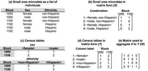
Statistical agencies collect small area microdata that contain individuals in n small areas who have d discrete attributes (e.g., sex and ethnicity) with a finite number of possible values. For example, the attribute of sex has two values: female and male. A combination is formed to contain one value from each of the d attributes, and the number of all possible combinations is denoted as m. For example, considering the two attributes of sex and ethnicity, there are four possible combinations (m = 4): <female, non-Hispanic>, <male, non-Hispanic>, <female, Hispanic>, and < male, Hispanic>. The small area microdata can be represented using an m × n matrix X = {x_kj}, where each element x_kj denotes the number of individuals in small area j (1 ≤ j ≤ n) who can be characterized by the attribute values in combination k (1 ≤ k ≤ m).

The original small area microdata (X) cannot be released because they contain individual information protected by privacy laws and regulations. Instead, aggregates from X are made available to the public. A primary source of these aggregates is census tables, such as those in the U.S. Census Summary File 1 (SF1; U.S. Census Bureau 2011) and the UK Census Local Characteristics (LC; Office for National Statistics 2013). Almost all types of census tables follow a similar structure. Each column of a census table is labeled with values from a subset of the d attributes. For example, if the small area microdata contain two attributes, sex and ethnicity, the table may only concern one of these attributes, sex, and it has two columns labeled < female > and < male>. Each cell in a table represents the number of individuals in a small area (row) who can be characterized by the attribute values labeled by a column (e.g., <female > or < male>). Assume that there is a total of q columns in these census tables. We represent these census tables using a q × n matrix Y = {y_ij}, where element y_ij represents the number of individuals in small area j (1 ≤ j ≤ n) who can be characterized by attribute values i (1 ≤ i ≤ q).

Small area microdata X can be transformed (i.e., aggregated) to census tables Y by premultiplying X with a q × m matrix W = {w_ik} (i.e., Y = WX), which expands as (1) $$y_{ij}=w_{i1}{x}_{1j}+w_{i2}{x}_{2j}+\cdots +w_{im}{x}_{mj},$$(1) where the value of w_ik is set to one when individuals counted in x_kj should be included in y_ij, and zero otherwise. Note that the value of w_ik can be determined without knowing the element values in X and Y; all we need to know is the purpose of the elements.

Figure 1 illustrates the three matrices X, Y, and W. In this example, small area microdata are collected for six individuals in two blocks (n = 2), and each individual has two attributes, sex and ethnicity (d = 2; Figure 1A). There are four possible combinations (m = 4) containing one value from each of these two attributes. An m × n = 4 × 2 matrix X is used to represent the small area microdata, as shown in Figure 1B. The small area microdata can be used to produce two public census tables (Figure 1C). These two census tables together have a total of four columns (q = 4), and a q × n = 4 × 2 matrix Y can be used to represent the census tables, where each census table is transposed and vertically stacked (Figure 1D). We construct a q × m = 4 × 4 matrix W to aggregate X to Y (Figure 1E). The first row of W, for example, is used to aggregate all females in a block and must set the first and third values to 1 (i.e., [1, 0, 1, 0]) because the first and third rows in X are where all females are counted.

Figure 1 An example used to illustrate X, Y, and W.

To the public, the values in X are unknown due to privacy constraints. The goal of this article is to develop a method that can be used for constructing SASM that can be aggregated to be as close to the published census tables as possible. The SASM are denoted as an m × n matrix X^′ = {x^′_kj} that has the same element meanings as X, but with each element being a decision variable to be determined so that the squared difference between synthetic (WX^′) and actual (Y) census tables is minimized: (2) $$\begin{array}{cc}\mathrm{m}\mathrm{in}& {\Vert \mathbf{W}{\mathbf{X}}^{\prime }-\mathbf{Y}\Vert }^2,\end{array}$$(2) (3) $$\begin{array}{cc}\text{subject to}& {x\prime }_{kj}\in {\mathbb{Z}}^{\mathrm{*}},\mathrm{ }\forall k,j,\end{array}$$(3) where the constraints in Equation 3(3) $$\begin{array}{cc}\text{subject to}& {x\prime }_{kj}\in {\mathbb{Z}}^{\mathrm{*}},\mathrm{ }\forall k,j,\end{array}$$(3) ensure integer decision variables. The optimization problem can be solved with integer programming solvers such as Gurobi, CPLEX, and COIN-OR.

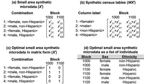
Figure 2 illustrates the process of generating the optimal SASM. We use an m × n = 4 × 2 matrix X^′ in Figure 2A to synthesize the small area microdata in Figure 1B. A synthetic census table in Figure 2B is generated by premultiplying X^′ with the same matrix W as in Figure 1E. We solve the optimization problem (Equations 2(2) $$\begin{array}{cc}\mathrm{m}\mathrm{in}& {\Vert \mathbf{W}{\mathbf{X}}^{\prime }-\mathbf{Y}\Vert }^2,\end{array}$$(2) and 3(3) $$\begin{array}{cc}\text{subject to}& {x\prime }_{kj}\in {\mathbb{Z}}^{\mathrm{*}},\mathrm{ }\forall k,j,\end{array}$$(3) ) and determine the optimal value of each element in X^′ (Figure 2C). The matrix X^′ is equivalent to a list of individuals in Figure 2D, which is how microdata are usually presented. In this example, the optimal SASM are not identical to the original small area microdata in Figure 1A. By minimizing the difference between the synthetic census tables (WX^′) and the published census tables (Y), however, the SASM retain statistics from the census tables and can still be considered realistic. We demonstrate this in the next section using actual census data.

Figure 2 An example of generating the optimal small area synthetic microdata (SASM).

Computational Experiments

Two counties in Ohio are selected as our study regions to reflect the diversity of demographic composition and population size in urban and rural areas. Franklin County is the most populous county in Ohio, with a total population of 1,163,414 in the 2010 Census, and it is urbanized and racially diverse. Guernsey County, in comparison, is largely rural and has a predominantly White population. It has a population of 40,087 in the 2010 Census, which makes it one of the least populous counties in Ohio.

We generate SASM for both counties. The SASM can be generated at any level of the published census tables (e.g., in the United States, they can be at the county, tract, block group, or block level). We choose the smallest level of geography, the block level, for demonstration purposes. Franklin County has 22,826 census blocks and Guernsey County has 3,768. Each individual in the SASM has five attributes: housing type, voting age, ethnicity, race, and sex (details of the possible values are given in Table A.1). There are a total of 4,032 possible combinations containing one value from each of these five attributes. Matrices used to represent the small area microdata (X) and the SASM (X^′) therefore have a size of 4,032 × 22,826 for Franklin County and 4,032 × 3,768 for Guernsey County. The SASM are generated by determining the element value in X^′ for each county.

To generate the SASM, we choose all eleven census tables from the 2010 U.S. Census SF1 that include population counts broken down by one or more of the five attributes at the census block level. These tables consist of a total of 308 columns (details referred to in Table A2). A 308 × 22,826 matrix Y is constructed to represent the census tables for Franklin County, and a 308 × 3,768 matrix Y is constructed for Guernsey County. The first row of matrix Y for each county, for example, contains the block-level population counts for non-Hispanic Whites (i.e., the first column in Table P5 of SF1; see Table A.2). We construct a 308 × 4,032 matrix W through which X can be aggregated to Y. The values in each row of W are set to aggregate the small area microdata or SASM to the appropriate row of Y. For example, the first row of W is used to aggregate all non-Hispanic Whites in each block, and we set its kth element (1 ≤ k ≤ 4,032) to one if individuals counted in the kth row of X are non-Hispanic Whites. Elements in the remaining rows of W have their values determined in a similar manner.

We use Gurobi (Gurobi Optimization 2021) as the optimization solver to determine the SASM. Using a computer with an Intel Core i7-6500U (2.5 GHz) processor and 8 GB RAM, the run times for Franklin and Guernsey Counties are 111 and 23 sec, respectively, which suggests the efficiency of the proposed method. The resulting SASM contain all 1,163,414 individuals in 22,826 census blocks of Franklin County and all 40,088 individuals in 3,768 census blocks of Guernsey County.

Technical Validation

To examine the validity of the SASM, we first perform internal validation to compare the synthetic census tables (WX^′) with the SF1 census tables involved in SASM generation. Specifically, we represent the eleven actual census tables listed in Table A.2 as a series of matrices Y₁, Y₂, · · ·, Y₁₁, where the pth (1 ≤ p ≤ 11) matrix Y_p = {y_pij} can be viewed as a transposition of census table p, with each matrix element y_pij denoting the number of individuals in small area j who can be characterized by the attribute values labeled by the ith column in table p. For example, Y₂ represents Table P8 of SF1, as listed in Table A.2, with its first row denoting the population count of Whites in each block. We obtain eleven matrices W₁, W₂, · · ·, W₁₁ that can be used to convert the small area microdata X to the eleven census tables Y₁, Y₂, · · ·, Y₁₁, respectively. The first row of matrix W₂, for example, is used to aggregate all Whites in each block and has its kth element set to one if individuals counted in the kth row of X are Whites. We calculate the sum of squared differences (d_p) between the pth synthetic (W_pX^') and actual (Y_p) census tables: (4) $$d_p={\Vert {\mathbf{W}}_p{\mathbf{X}}^{\prime }-{\mathbf{Y}}_p\Vert }^2.$$(4)

A value of d_p equal to zero indicates that the SASM perfectly preserve the information from census tables for every small area. In our experiments for both counties, the value of d_p is zero for all eleven tables examined. In other words, the synthetic census tables are identical to the actual tables. This indicates that information from the census tables is preserved by the SASM.

External validation is conducted to compare the SASM (X^′) with external data that are not involved in SASM generation. Because true census small area microdata are not publicly available, sample microdata from the ACS PUMS are used for comparison. Each calendar year, the U.S. Census Bureau produces one-year and five-year ACS PUMS data that, respectively, represent a 1 and 5 percent sample of the national population. We use the unweighted sample from the 2010 5-Year ACS PUMS because it is the largest sample microdata set that can be used for comparison. Each individual in the ACS PUMS has four of the five SASM attributes, including age, ethnicity, race, and sex, as well as others that are not presented in the SASM (e.g., citizenship status). For the attribute race, it only has seven possible values because the fifty-seven combinations of races (as shown in Table A.1) are grouped as one value. The smallest geographic unit in the ACS PUMS is the Public Use Microdata Area (PUMA), which typically contains a group of counties or census tracts and has a population of no less than 100,000 people (U.S. Census Bureau 2021). Franklin County has eleven PUMAs, while Guernsey County is included with Holmes and Coshocton Counties in one PUMA (Figure A.1). To test the effect of unmatched boundaries between Guernsey County and the PUMA on validation results, we also generate the SASM for Holmes and Coshocton using the same procedures as described previously for Franklin and Guernsey. The SASM for Franklin, Guernsey, and Guernsey-Holmes-Coshocton are compared to the sample microdata in the corresponding PUMAs.

To make the comparisons, we first remove attributes from the sample microdata that are not included in the SASM. We also remove the housing type from the SASM as it is not contained in the sample microdata. For the remaining four attributes (voting age, ethnicity, race, and sex), there are 2 × 2 × 7 × 2 = 56 possible combinations containing one value from each of these attributes. We use a 56-dimension row vector a = {a_k} to represent the sample microdata for each PUMA in Franklin County as well as the PUMA that contains Guernsey County. Each element a_k denotes the number of individuals in a PUMA who can be characterized by the attribute values in combination k (1 ≤ k ≤ 56). We summarize each individual in the block-level SASM to the PUMA that the person falls into, and then represent the data using a 56-dimension row vector b = {b_k}. Each element b_k has the same meaning as a_k except that it refers to a population count from the SASM instead of from the sample microdata. Cosine similarity (Dangeti 2017) is used to determine the similarity between the sample microdata (a) and the SASM (b) for each PUMA. Because the sample microdata only includes a subset of the population from the true small area microdata, elements in a are always smaller or equal to their correspondents in b. The use of cosine similarity enables measuring similarity regardless of magnitude. 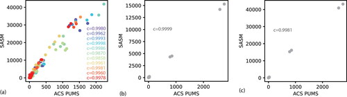The cosine similarity is expressed as (5) $$c=\frac{{\mathrm{a}}^T\mathrm{b}}{\Vert \mathrm{a}\Vert \mathrm{ }\Vert \mathrm{b}\Vert },$$(5) where ǁ·ǁ is an operator that calculates the Euclidean norm of the input vector. The value of c ranges from −1 to 1, with 1 indicating that the two sets of data are exactly alike and 0 denoting no similarity. Figure 3 illustrates the cosine similarity between the SASM and the ACS PUMS for each PUMA. The cosine similarity for Franklin County is above 0.995 in nine out of the eleven PUMAs and above 0.985 in the remaining two. The cosine similarity values for Guernsey and Guernsey-Holmes-Coshocton are greater than 0.995 when comparing the corresponding SASM with the ACS PUMS in the same PUMA. These findings imply that the SASM can well represent the real population in the sample microdata.

Figure 3 Comparisons between the small area synthetic microdata (SASM) and the American Community Survey Public Use Microdata Sample (ACS PUMS) in each Public Use Microdata Area (PUMA). (A) Franklin County, (B) Guernsey County, and (C) Guernsey-Holmes-Coshocton Counties. Each dot represents a data point formed by values in the ACS PUMS and the SASM. Eleven colors are used for dots in (A), each representing a PUMA in Franklin County.

Case Study I: Demographic Mapping in Data-Scarcity Scenarios

We now demonstrate how the SASM can be used in demographic mapping to overcome data scarcity. Demographic mapping often requires data on population attributes at small area levels. One possible data source is the complete individual-level census responses, but they have restrictive access policies for protecting individual privacy. Public data sources include aggregated data and sample microdata, but these data lack certain small area information. For example, census tables from the SF1 do not include population counts or percentages by the combination of voting age, ethnicity, and race. Although the population percentages can be found from sample microdata such as the PUMS, they are not available at the small area level (e.g., the block level). If mapping these counts or percentages at the small area level is required, it cannot be done using existing public data.

Data scarcity in demographic mapping can be addressed with SASM. Specifically, the SASM (X′) generated for Franklin and Guernsey Counties can be used to produce maps of block-level population percentages by the combination of voting age, ethnicity, and race. To produce such maps, a new matrix W′ is constructed to aggregate the SASM X′ to block-level population counts broken down by the three attributes. As listed in Table A.2, there are 8 × 2 × 2 × 63 × 2 = 4,032 combinations that contain one value from each of all five SASM attributes, and there are 2 × 2 × 63 = 252 combinations that contain one value from each of the attributes of voting age, ethnicity, and race. The matrix W′ thus has a size of 252 × 4,032, with each row used to count the number of individuals characterized by a combination of attribute values for voting age, ethnicity, and race. The population percentages can then be calculated by dividing the population counts by the population totals in each block.

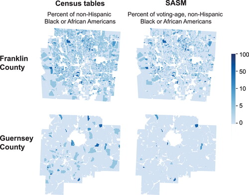
Figure 4 illustrates the maps of block-level percentages of the voting-age, non-Hispanic Black or African American population derived from the SASM. We also present the closest block-level maps that can be produced from published census tables (i.e., maps of block-level percentages of the non-Hispanic Black or African American population). Compared to maps generated using published census tables, those from the SASM provide a detailed breakdown of the population percentages and are able to show an age-specific spatial pattern. For example, maps from the SASM show low percentages of voting-age, non-Hispanic Black or African Americans in the southwest of Guernsey County. This pattern is masked in maps generated using census tables due to the lack of age-specific information.

Figure 4 Mapping the block-level population percentages derived from published census tables and the small area synthetic microdata (SASM). The north-central region of Guernsey County is the Salt Fork State Park, which has zero population.

Case Study II: Replicating Differential Privacy for the 2020 U.S. Census

We provide an example of using the SASM for replicating and examining a privacy protection mechanism—known as differential privacy—used in the 2020 U.S. Census (Abowd 2018). Differential privacy requires adding statistical noise to all published census tables for protecting individual privacy, and the ability to replicate such a mechanism allows researchers and data users to quantify its effects on data utility (Santos-Lozada, Howard, and Verdery 2020; Kenny et al. 2021). To replicate the differential privacy mechanism, small area microdata are needed to be used as the data input, but such data are not publicly available due to confidentiality constraints. The SASM can be used instead as the input to resolve this issue.

We implement the differential privacy mechanism on the SASM for Franklin and Guernsey Counties using the computer source code released by the U.S. Census Bureau (2020). A set of differentially private SASM called DP-SASM are generated. The DP-SASM can be aggregated to produce the population counts or percentages by a subset of attributes (e.g., race only) and at a different geographic level (e.g., block group or tract level). These counts and percentages correspond to the aggregated data in a census table to which the general public has access. For the sake of illustration, we present examples of such data using the tract-level percentages of Black or African Americans in Franklin and Guernsey Counties, as shown in Figure 5. Because differential privacy requires adding noise for privacy protection, we compare the percentages from the original SASM and DP-SASM and examine the impact of differential privacy on the utility of data. For each tract, we measure data utility by quantifying the discrepancy between the percentages from SASM (p_SASM) and DP-SASM (p_DP-SASM) using a metric called percent error (PE): (6) $$\text{PE}=\frac{\left|p_{\text{SASM}}-p_{\text{DP}-\text{SASM}}\right|}{p_{\text{SASM}}+p_{\text{DP}-\text{SASM}}}\mathrm{ }\times 100\mathrm{\%}.$$(6)

Figure 5 Tract-level population percentages calculated with small area synthetic microdata (SASM) and differentially private SASM (DP-SASM), as well as their percent error (PE). For each county, the percentages that correspond to the highest value of PE are labeled.

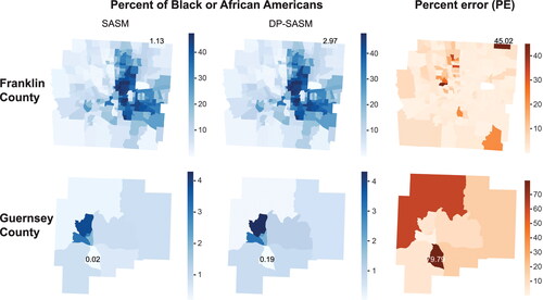
The value of PE ranges between 0 and 100 percent. A PE of 0 percent denotes no discrepancy between the two sets of percentages and thus the highest data utility, whereas a PE of 100 percent indicates the opposite. As shown in Figure 5, areas with low percentages of Black or African Americans tend to have high values of PE and thus low data utility. Particularly in Guernsey County, tracts with a percentage of Black or African Americans less than 1 percent have their PE higher than 60 percent. These findings suggest that the impact of differential privacy on data utility varies spatially and can be significant in areas with specific demographic structures. As this mechanism is used in census data production that will affect numerous applications of census data, it should be improved to better preserve data utility while protecting privacy.

Discussion and Conclusions

Providing useful spatial data without compromising individual privacy is a critical challenge in geographical research (Armstrong and Ruggles 2005; Richardson et al. 2015; Kamel Boulos et al. 2022). A typical example is small area microdata, which contain spatially detailed individual-level information and has a wide range of applications. Such data, however, are rarely made public because of privacy concerns. This article proposes an optimization method for generating public-use SASM using entirely public census tables. Our computational experiments show that the proposed method is effective in generating realistic data that represents the real population and is also computationally efficient to derive optimal SASM. Compared with existing methods for generating SASM (e.g., synthetic reconstruction and combinatorial optimization), the proposed method does not require a predefined order to append attributes to each individual, nor does it rely on specific sample microdata to make imputations. Instead, our method only requires a set of census tables that are publicly available in many countries as input to provide effective results. Along with the source code provided, we are able to ensure the generality and reusability of this method. One limitation of this research is that the actual census small area microdata cannot be directly compared to our data for validation because it is not made available to the general public. Simulated population data can be used in the future to evaluate the effectiveness of the proposed approach. Other synthetic data sources (Grefenstette et al. 2013) can also be used to test the method.

Our research also reveals a potential problem with the census tables: It is possible to reconstruct the original small area microdata if sufficient aggregated information is published in the census tables. This risk of the census tables is described by the fundamental law of information recovery (Dinur and Nissim 2003), which states, informally, that publishing too many aggregated data can completely reveal the underlying microdata. In 2018, the U.S. Census Bureau conducted internal experiments that sought to determine the census block, age, sex, race, and Hispanic origin of the U.S. population using 6.2 billion statistics from seventeen tables published as part of the 2010 Census (Abowd 2021). In these experiments, the attributes of each person living in a block are treated as a collection of decision variables, and a set of constraints is extracted from the published tables. Optimization problems are then formulated to determine the values of the set of attributes so that the reconstructed microdata can satisfy the constraints (Garfinkel, Abowd, and Martindale 2019). Our method, which generates synthetic data using public census tables, can possibly be used to reconstruct the original microdata, as done in the Census Bureau’s experiments. The Census Bureau’s method and ours both use optimization, but instead of listing all individual records, we develop a matrix representation for the microdata. The number of decision variables is thus determined by the number of attributes for each individual, rather than the total number of individuals. In our case, when the number of attributes is fixed, the time required to solve the optimization problem will not significantly increase in areas with large population sizes, compared to the Census Bureau’s method.

The possibility of reconstruction using the current release of census tables is subject to debate, though. The Census Bureau states that its reconstruction experiments confirm correct reidentifications for 52 million people in the United States (17 percent of the 2010 Census resident population) by matching its reconstructed microdata against commercial data from 2010 (Abowd 2021). A large body of literature also demonstrates, however, that the Census Bureau’s reconstruction is only one instance of reconstruction to match the census tables, and that the proportion of correct reidentifications could be explained by chance (Muralidhar 2022; Ruggles and Van Riper 2022). It is true that certain individuals in the synthetic microdata will, in some cases, be the same as those in the true small area microdata (e.g., the first two individuals in Figure 1A and Figure 2D). Most individuals in the synthetic microdata, though, will not match anyone in the real world, and an external attacker has no means of confirming whether there is a match (U.S. Census Bureau 2019). Because of this uncertainty, any attacker attempting to use synthetic data to reveal the identities of census respondents should find it practically impossible.

The past three decades have witnessed the emergence of large-scale and complex models and platforms for spatial microsimulation (Birkin and Clarke 2011; Tanton and Edwards 2012) and agent-based modeling (Eubank et al. 2004), such as the Los Alamos National Laboratory’s TRansportation ANalysis SIMulation System (TRANSIMS; Smith, Beckman, and Baggerly 1995) and the European Union’s tax-benefit microsimulation model (EUROMOD; Sutherland and Figari 2013). Making the most of these tools demands microdata inputs with high levels of detail, particularly in the geographic locations of individuals. Specifically, individuals in the microdata are expected to have address-level or coordinate-level point locations rather than only the spatial units (Chapuis et al. 2018). Although our method does not assign point locations to individuals, some recent progress has the potential to address this limitation. Data sets that reveal population distribution at a fine resolution are becoming increasingly available in North America and even on a global scale. For example, the LandScan Global Population Data (Bhaduri et al. 2007) provides global population counts at a resolution of 30 arc seconds (roughly 1 km). In addition, open building footprint data, such as the Microsoft Building Footprint Data (Microsoft 2018), can be used to inform potential point locations of individuals. A combination of these results is promising to further process the SASM for generating the microdata with reliable point locations, which can be used to provide data support for models of high complexity.

Acknowledgment

The synthetic data and code are available in GitHub at https://github.com/linyuehzzz/synthetic-populations.

Additional information

Notes on contributors

Yue Lin

YUE LIN is a PhD Candidate in the Department of Geography, Ohio State University, Columbus, OH 43210. E-mail: [email protected]. Her research interests include spatial data science, geocomputation, and digital privacy.

Ningchuan Xiao

NINGCHUAN XIAO is Professor in the Department of Geography, Ohio State University, Columbus, OH 43210. E-mail: [email protected]. His research interests include spatial decision support systems, cartography, environmental and ecological modeling, and Web-based geographic information systems.

Appendix

Table A.1 shows the five attributes in the SASM and their potential values. Table A.2 presents the eleven census tables selected to construct the SASM. Figure A.1 shows the boundaries of PUMAs and counties.

Figure A.1 Boundaries of Public Use Microdata Areas (PUMAs) (black) and counties (gray) in Ohio. Franklin County includes 11 PUMAs (center, colored in blue), and (A) Guernsey, (B) Holmes, and (C) Coshocton counties collectively make up one PUMA (east, colored in blue).

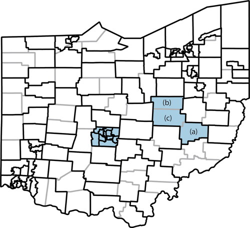
Table A.1 Attributes in the small area synthetic microdata (SASM)

Attribute	Range of values	No. of possible values
Housing type	Household and seven group quarter types (Correctional facilities for adults, Juvenile facilities, Nursing facilities/skilled-nursing facilities, Other institutional facilities, College/university student housing, Military quarters, Other noninstitutional facilities)	8
Voting age	Age < 18 and age ≥ 18	2
Ethnicity	Of Hispanic origin and non-Hispanic.	2
Race	Six single races (White, Black or African American, American Indian or Alaska Native, Asian, Native Hawaiian or other Pacific Islander, Some other race) and 57 possible combinations of these six races (for details see the 2010 Census Summary File 1 Technical Documentation, 6–24).	63
Sex	Male and female	2

Table A.2 Tables from the 2010 U.S. Census Summary File 1 to construct the small area synthetic microdata (SASM)

Table no.	Description	No. of columns
P5	Population counts broken down by ethnicity by race	126
P8	Population counts broken down by race	63
P9	Population counts broken down by race for non-Hispanics	63
P43	Population counts broken down by sex by age by group quarter types	28
P12A	Population counts broken down by sex by age for Whites	4
P12B	Population counts broken down by sex by age for Black or African Americans	4
P12C	Population counts broken down by sex by age for American Indian or Alaska Natives	4
P12D	Population counts broken down by sex by age for Asians	4
P12E	Population counts broken down by sex by age for Native Hawaiian or other Pacific Islanders	4
P12F	Population counts broken down by sex by age for individuals with some other race alone	4
P12G	Population counts broken down by sex by age for individuals with two or more races	4

Literature Cited

- Abowd, J. M. 2018. The US Census Bureau adopts differential privacy. In Proceedings of the 24th ACM SIGKDD International Conference on Knowledge Discovery & Data Mining, 2867. New York: ACM.
- Abowd, J. M. 2021. 2010 Supplemental declaration of John M. Abowd, State of Alabama v. United States Department of Commerce, Case No. 3:21-CV-211-RAH-ECM-KCN.
- Alessandretti, L. 2022. What human mobility data tell us about COVID-19 spread. Nature Reviews Physics 4 (1):12–13.
- Armstrong, M. P., and A. J. Ruggles. 2005. Geographic information technologies and personal privacy. Cartographica: The International Journal for Geographic Information and Geovisualization 40 (4):63–73. doi: 10.3138/RU65-81R3-0W75-8V21.
- Bansal, M. A., D. R. Sharma, and D. M. Kathuria. 2022. A systematic review on data scarcity problem in deep learning: Solution and applications. ACM Computing Surveys 54 (10s):1–29. doi: 10.1145/3502287.
- Beckman, R. J., K. A. Baggerly, and M. D. McKay. 1996. Creating synthetic baseline populations. Transportation Research Part A: Policy and Practice 30 (6):415–29. doi: 10.1016/0965-8564(96)00004-3.
- Bhaduri, B., E. Bright, P. Coleman, and M. L. Urban. 2007. LandScan USA: A high-resolution geospatial and temporal modeling approach for population distribution and dynamics. GeoJournal 69 (1–2):103–17. doi: 10.1007/s10708-007-9105-9.
- Birkin, M., and M. Clarke. 1988. Synthesis—A synthetic spatial information system for urban and regional analysis: Methods and examples. Environment and Planning A: Economy and Space 20 (12):1645–71. doi: 10.1068/a201645.
- Birkin, M., and M. Clarke. 1989. The generation of individual and household incomes at the small area level using synthesis. Regional Studies 23 (6):535–48. doi: 10.1080/00343408912331345702.
- Birkin, M., and M. Clarke. 2011. Spatial microsimulation models: A review and a glimpse into the future. In Population dynamics and projection methods: Understanding population trends and processes, ed. J. Stillwell and M. Clarke, 193–208. Dordrecht, The Netherlands: Springer.
- Chapuis, K., P. Taillandier, M. Renaud, and A. Drogoul. 2018. Gen*: A generic toolkit to generate spatially explicit synthetic populations. International Journal of Geographical Information Science 32 (6):1194–1210. doi: 10.1080/13658816.2018.1440563.
- Dangeti, P. 2017. Statistics for machine learning. Birmingham, UK: Packt Publishing.
- Dinur, I., and K. Nissim. 2003. Revealing information while preserving privacy. In Proceedings of the Twenty-Second ACM SIGMOD-SIGACT-SIGART Symposium on Principles of Database Systems, 202–10. New York: ACM. doi: 10.1145/773153.773173.
- Domingo-Ferrer, J. 2009. Synthetic microdata. In Encyclopedia of database systems, ed. L. Liu and M. T. Ozsu, 2899–2900. Boston, MA: Springer.
- Eubank, S., H. Guclu, V. Anil Kumar, M. V. Marathe, A. Srinivasan, Z. Toroczkai, and N. Wang. 2004. Modelling disease outbreaks in realistic urban social networks. Nature 429 (6988):180–84. doi: 10.1038/nature02541.
- Ferguson, N. M., D. A. Cummings, S. Cauchemez, C. Fraser, S. Riley, A. Meeyai, S. Iamsirithaworn, and D. S. Burke. 2005. Strategies for containing an emerging influenza pandemic in southeast Asia. Nature 437 (7056):209–14. doi: 10.1038/nature04017.
- Garfinkel, S., J. M. Abowd, and C. Martindale. 2019. Understanding database reconstruction attacks on public data. Communications of the ACM 62 (3):46–53. doi: 10.1145/3287287.
- Gonzalez, M. C., C. A. Hidalgo, and A.-L. Barabasi. 2008. Understanding individual human mobility patterns. Nature 453 (7196):779–82. doi: 10.1038/nature06958.
- Goodman, S. N., D. Fanelli, and J. P. Ioannidis. 2016. What does research reproducibility mean? Science Translational Medicine 8 (341):341ps12. doi: 10.1126/scitranslmed.aaf5027.
- Grefenstette, J. J., S. T. Brown, R. Rosenfeld, J. DePasse, N. T. Stone, P. C. Cooley, W. D. Wheaton, A. Fyshe, D. D. Galloway, A. Sriram, et al. 2013. Fred (a framework for reconstructing epidemic dynamics): An open-source software system for modeling infectious diseases and control strategies using census-based populations. BMC Public Health 13 (1):1–14. doi: 10.1186/1471-2458-13-940.
- Gurobi Optimization. 2021. Gurobi Optimizer reference manual. Accessed September 22, 2022. https://www.gurobi.com.
- Haibe-Kains, B., G. A. Adam, A. Hosny, F. Khodakarami, L. Waldron, B. Wang, C. McIntosh, A. Goldenberg, A. Kundaje, C. S. Greene, et al. 2020. Transparency and reproducibility in artificial intelligence. Nature 586 (7829):E14–E16. doi: 10.1038/s41586-020-2766-y.
- Hermes, K., and M. Poulsen. 2012. A review of current methods to generate synthetic spatial microdata using reweighting and future directions. Computers, Environment and Urban Systems 36 (4):281–90. doi: 10.1016/j.compenvurbsys.2012.03.005.
- Huang, Z., and P. Williamson. 2001. A comparison of synthetic reconstruction and combinatorial optimisation approaches to the creation of small-area microdata. Tech. Rep. Department of Geography, University of Liverpool, Liverpool, UK.
- IPUMS. 2022. Project overview—IPUMS International. Accessed September 22, 2022. https://international.ipums.org/international/overview.shtml#page-title.
- Kamel Boulos, M. N., M.-P. Kwan, K. El Emam, A. L.-L. Chung, S. Gao, and D. B. Richardson. 2022. Reconciling public health common good and individual privacy: New methods and issues in geoprivacy. International Journal of Health Geographics 21 (1):1–9. doi: 10.1186/s12942-022-00300-9.
- Kenny, C. T., S. Kuriwaki, C. McCartan, E. T. Rosenman, T. Simko, and K. Imai. 2021. The use of differential privacy for census data and its impact on redistricting: The case of the 2020 US Census. Science Advances 7 (41):eabk3283. doi: 10.1126/sciadv.abk3283.
- Lin, Y., and N. Xiao. 2022. Developing synthetic individual-level population datasets: The case of contextualizing maps of privacy-preserving census data. Paper presented at AutoCarto 2022, the 24th International Research Symposium on Cartography and GIScience, November 2-4, Redlands, CA, USA.
- Lin, Y., and N. Xiao. 2023. A computational framework for preserving privacy and maintaining utility of geographically aggregated data: A stochastic spatial optimization approach. Annals of the American Association of Geographers, 1–22. Advance online publication. doi: 10.1080/24694452.2023.2178377.
- Lovelace, R., M. Dumont, R. Ellison, and M. Zalǒznik. 2017. Spatial microsimulation with R. New York: Chapman Hall/CRC.
- Matthews, G. J., and O. Harel. 2011. Data confidentiality: A review of methods for statistical disclosure limitation and methods for assessing privacy. Statistics Surveys 5:1–29. doi: 10.1214/11-SS074.
- Microsoft. 2018. Microsoft building footprint data. Accessed June 13, 2018. https://github.com/microsoft/USBuildingFootprints.
- Mitton, L., H. Sutherland, and M. Weeks. 2000. Microsimulation modelling for policy analysis: Challenges and innovations. Cambridge, UK: Cambridge University Press.
- Muralidhar, K. 2022. A re-examination of the Census Bureau reconstruction and reidentification attack. In Privacy in statistical databases. PSD 2022. Lecture notes in computer science, vol. 13463, ed. J. Domingo-Ferrer and M. Laurent. Springer, Cham. doi: 10.1007/978-3-031-13945-1_22.
- Office for National Statistics. 2013. Local characteristics. Accessed September 22, 2022. https://www.ons.gov.uk/census/2011census/2011censusdata/2011censusdatacatalogue/localcharacteristics.
- P’erignon, C., K. Gadouche, C. Hurlin, R. Silberman, and E. Debonnel. 2019. Certify reproducibility with confidential data. Science 365 (6449):127–28. doi: 10.1126/science.aaw2825.
- Richardson, D. B., M.-P. Kwan, G. Alter, and J. E. McKendry. 2015. Replication of scientific research: Addressing geoprivacy, confidentiality, and data sharing challenges in geospatial research. Annals of GIS 21 (2):101–10. doi: 10.1080/19475683.2015.1027792.
- Ruggles, S. 2014. Big microdata for population research. Demography 51 (1):287–97. doi: 10.1007/s13524-013-0240-2.
- Ruggles, S., R. McCaa, M. Sobek, and L. Cleveland. 2015. The IPUMS collaboration: Integrating and disseminating the world’s population microdata. Journal of Demographic Economics 81 (2):203–16. doi: 10.1017/dem.2014.6.
- Ruggles, S., and D. Van Riper. 2022. The role of chance in the Census Bureau database reconstruction experiment. Population Research and Policy Review 41 (3):781–88. doi: 10.1007/s11113-021-09674-3.
- Santos-Lozada, A. R., J. T. Howard, and A. M. Verdery. 2020. How differential privacy will affect our understanding of health disparities in the United States. Proceedings of the National Academy of Sciences of the United States of America 117 (24):13405–12. doi: 10.1073/pnas.2003714117.
- Slavkovic, A., S. Kinney, and A. Karr. 2011. O privacy, where art thou? Research access to restricted-use data. CHANCE 24 (4):41–45. doi: 10.1080/09332480.2011.10739886.
- Smith, L., R. Beckman, and K. Baggerly. 1995. TRANSIMS: Transportation analysis and simulation system. Tech. Rep., Los Alamos National Lab, Los Alamos, NM.
- Sutherland, H., and F. Figari. 2013. EUROMOD: The European Union tax-benefit microsimulation model. International Journal of Microsimulation 6 (1):4–26. doi: 10.34196/ijm.00075.
- Tanton, R., and K. Edwards. 2012. Spatial microsimulation: A reference guide for users. Dordrecht, The Netherlands: Springer Science & Business Media.
- Tranmer, M., A. Pickles, E. Fieldhouse, M. Elliot, A. Dale, M. Brown, D. Martin, D. Steel, and C. Gardiner. 2005. The case for small area microdata. Journal of the Royal Statistical Society Series A: Statistics in Society 168 (1):29–49. doi: 10.1111/j.1467-985X.2004.00334.x.
- U.S. Census Bureau. 2011. 2010 United States Census summary file 1 dataset. Accessed September 22, 2022. https://www.census.gov/data/datasets/2010/dec/summary-file-1.html.
- U.S. Census Bureau. 2019. Census Bureau adopts cutting edge privacy protections for 2020 Census. Accessed September 22, 2022. https://www.census.gov/newsroom/blogs/random-samplings/2019/02/census bureau adopts.html.
- U.S. Census Bureau. 2020. Das 2010 demonstration data products disclosure avoidance system release. Accessed September 22, 2022. https://github.com/uscensusbureau/census2020-das-2010ddp.
- U.S. Census Bureau. 2021. Understanding and using the American Community Survey Public Use Microdata sample files. Accessed September 22, 2022. https://www.census.gov/content/dam/Census/library/publications/2021/acs/acs_pums_handbook_2021.pdf.
- Voas, D., and P. Williamson. 2000. An evaluation of the combinatorial optimisation approach to the creation of synthetic microdata. International Journal of Population Geography 6 (5):349–66. doi: 10.1002/1099-1220(200009/10)6:5<349::AID-IJPG196>3.0.CO;2-5.
- Williamson, P., M. Birkin, and P. H. Rees. 1998. The estimation of population microdata by using data from small area statistics and samples of anonymised records. Environment & Planning A 30 (5):785–816. doi: 10.1068/a300785.
Appendix
shows the five attributes in the SASM and their potential values. presents the eleven census tables selected to construct the SASM. shows the boundaries of PUMAs and counties.