Investment subsidies and regional welfare: a dynamic framework and its application to the European regional policy

ABSTRACT

This paper focuses on the question of the effectiveness of subsidies to private and public investment, which are a key component of European regional policy. Given mixed findings from empirical studies, it is worth studying this issue in a simulation model, where the results can be traced back to policy shocks and model assumptions. To this end, the paper employs a multiregional dynamic framework with a perfectly integrated capital market. It is found that investment subsidies are effective and capital market spillover effects are small. The argument is illustrated by numerical simulations of actual investment subsidies to the European Union regions.

KEYWORDS:

• investment subsidies
• European Union regional policy
• forward-looking dynamics
• semi-endogenous growth
• interregional capital flows

JEL:

• H71
• O41
• R13
• R58

INTRODUCTION

Both in the European Union (EU) and in European countries in general, subsidizing investment in lagging regions is the most important regional policy instrument (European Union, 2017). From the theory point of view, investment subsidies are mainly seen as an instrument for strengthening regional economic activity and boosting economic growth (Barro & Sala-i-Martin, 1995). As a support instrument, they can be a more efficient policy than other alternatives, for example, employment subsidies (Fuest & Huber, 2000). Furthermore, investment subsidies can play a role in international tax competition by increasing the incentives for firms to invest and to settle in certain locations (Baldwin, Forslid, Martin, Ottaviano, & Robert-Nicoud, 2003). These theoretical results predict that investment subsidies should generate welfare gains in the target regions. However, the magnitude of these effects and their dependence on various local factors remains a highly relevant policy issue (Piattoni & Polverari, 2016).

The empirical literature on the effects of regional subsidies (in particular, EU Structural Funds) is quite large, including applications of simulation models (Brandsma, Kancs, Monfort, & Rillaers, 2015; Garau & Lecca, 2015; Ribeiro, Domingues, Perobelli, & Hewings, 2018), case studies (Huggins, 1998; Lolos, 1998) and econometric analyses (Cerqua & Pellegrini, 2014; Dall’erba & Le Gallo, 2008; de Castris & Pellegrini, 2012). In terms of the effectiveness of regional subsidies (ability to produce positive economic impacts in the target regions), the findings from econometric studies and case studies are ambiguous due to the use of different methods, varying sample sizes and different time periods. They range from no significant effects of regional funds to large and positive impacts on the regions supported (Dall’erba & Le Gallo, 2008; Fratesi, 2016).

One reason that suggests itself for the more pessimistic findings might be that investment subsidies are not specific enough to concentrate aid on the regions that are lagging behind most because the benefits trickle down to other places and ultimately little is left for the regions earmarked for support. Two channels likely to transmit benefits to places not initially selected for support are trade and the capital market. Through the trade channel the demand impulse generated by a subsidy will in part spread to the rest of the world. Repercussions on the capital market derive from the fact that subsidies for private capital will affect stock prices. They make capital more abundant in the supported regions and thus depress its market value. If people in the supported regions happen to own these capital stocks, they could suffer from an asset loss. However, apart from the routine procedure of correcting for ‘spatial effects’ in the econometric studies (Fratesi, 2016), these spillover effects and transmission mechanisms potentially diverting desired impacts away from the targeted regions have not received much attention so far in the empirical literature.

Given these mixed findings and research gaps, it is worth studying the effects of investment subsidies with the help of simulation models, where the results can be clearly traced back to the shocks and the model assumptions. Recent multiregional modelling approaches such as GMR (Varga, 2017) and RHOMOLO (Di Comite, Lecca, Monfort, Persyn, & Piculescu, 2018) would enhance our understanding of the causal chains linking regional investments and their spatial impacts. However, their applications have not so far focused on effectiveness, efficiency and spillover effects. This paper addresses this research gap using a stylized multiregional model, which is calibrated using data for a set of European regions. The application of the model is not meant to be a comprehensive impact assessment of EU regional policy impacts. Instead, it focuses on the effectiveness and efficiency of investment subsidies under different model assumptions. The policy issue addressed here is that of checking how regional welfare effects compare with the size of the subsidies and to what extent interregional spillovers play a role.

With a static model incorporating agglomeration externalities and perfect capital stock mobility, Dupont and Martin (2006) argue that regional capital subsidies may increase inequality, thus harming poor regions. Their framework, however, overlooks several important features of the actual policies. First, in practice subsidies support new investment projects and not the existing capital stock. Second, much of the actual regional support focuses on public, rather than private capital. Third, investment is a dynamic phenomenon resulting from intertemporal trade-offs, which cannot be properly reflected in a static framework. Both public and private regional capital need time to accumulate and to generate impacts. A dynamic approach is therefore needed to study the impact of capital mobility in an appropriate way.

A recent approach suitable for studying the effects of regional subsidies is the dynamic spatial computable general equilibrium (CGE) modelling framework (Bröcker & Korzhenevych, 2013). Dynamic spatial CGE models are rare and usually recursive, meaning that static solutions in each period are connected with each other using ad-hoc dynamic transition rules. In contrast, the approach in this paper is to apply a fully forward-looking model, which allows for consistent saving and investment decisions and a proper welfare analysis.

The present paper thus studies regional investment subsidies in a multiregional neoclassical dynamic framework. We set up a model with trade in heterogeneous goods, with a perfectly integrated financial capital market and sluggish adjustment of private and public regional capital stocks. Consumers and investors act under perfect foresight. We derive the equilibrium system, show how to solve it and simulate EU regional subsidies for private and public capital in computational applications. We infer the degree of effectiveness of the policy by comparing the welfare gain generated by investment subsidies with the hypothetical scenario of a lump-sum transfer. An alternative regional set-up and an alternative demand structure for traded goods are used to check the robustness of the results.

The results of the paper are the following. First, we show that a spatial forward-looking CGE model is an operational tool that can be used to answer policy questions. Second, in terms of stylized policy application we can answer several questions about the investment subsidies. We show that this instrument is at least weakly effective (it produces a positive welfare effect in the target regions). The size of the welfare effect is close to the size of regional support. The target regions gain more through a subsidy to private capital than through a lump-sum transfer (what we refer to as strong effectiveness below). We show that subsidies can lead to a welfare loss for the EU as a whole and that they lead to welfare losses in the rest of the world in all scenarios. The findings are based on a theoretically consistent dynamic multiregional set-up and are robust to various regional aggregation settings.

THE FORMAL MODEL

The model presented here is a dynamic spatial computable general equilibrium (DSpCGE) model for a closed system of regions. In our empirical application, this system covers the whole world, while the policy under study is executed by just a small part of the world: the EU. For each region, the basic set-up is an open-economy version of the Ramsey optimal savings model, combined with an investment adjustment costs framework (Abel & Blanchard, 1986). Thus, both households and firms make intertemporal decisions and have perfect foresight. The specification of the production and household sectors and the goods markets is close to an earlier static model (Bröcker, 1998). The functions of the state sector are restricted to tax collection, subsidy payments and public capital provision. The policy simulations describe regional subsidies or transfers financed by a tax collected at a supranational level. The model is set up in continuous time t in years, running from zero to infinity. To avoid notational clutter, we usually suppress both the time argument and the regional subscript. Calligraphic symbols represent real quantities in contradistinction to nominal variables, which are given in standard italics.

Firms

Identical firms located in the region produce output $\mathcal{M}$ using a Cobb–Douglas (CD) technology by combining public capital $\mathcal{G}$, private capital $\mathcal{K}$, effective amount of labour service $\mathcal{L}$, local goods $\mathcal{H}$ and a constant elasticity of substitution (CES) composite of tradable goods $\mathcal{F}$ (coming from all regions):(1) $\mathcal{M}=\varphi {\mathcal{G}}^{\lambda }{\mathcal{L}}^{\alpha }{\mathcal{K}}^{\text{β}}{\mathcal{H}}^{\gamma }{\mathcal{F}}^{\eta },$(1) where $\varphi$ is the regional productivity parameter; and $\alpha +\text{β}+\gamma +\eta =1$. The term ${\mathcal{G}}^{\lambda }$ represents the impact of the public capital stock. It is free and exerts a positive externality on the firm. The production function exhibits constant returns to scale at both the firm level and for the entire region. However, private and social partial elasticities differ due to the externality. The joint social partial production elasticity of the two types of capital is $\text{β}+\lambda$, while the private partial production elasticity of capital is only $\text{β}$.

The regional population is assumed to be immobile and constant at $\overline{\mathcal{L}}$. The effective amount of labour input is assumed to grow at an exogenous rate of technological progress, $\tilde{\xi }$, that is:(2) ${\mathcal{L}}_r\left(t\right)=\overline{{\mathcal{L}}_r}\exp \left(\tilde{\xi }t\right)$(2) Firms not only produce but also invest. To add gross investment $\mathcal{I}$ to the existing capital stock, they need $\mathcal{I}\left(1+\left(\zeta /2\right)\left(\mathcal{I}/\mathcal{K}\right)\right)$ units of investment goods. The ‘first unit’ of investment goods is transformed one-to-one to installed capital. If capital grows, however, more than one unit of the investment good per unit of new capital installed is required, and the input requirement per unit of new capital becomes larger with the larger growth rate. This increase is the stronger, the larger the adjustment cost parameter $\zeta$. For the sake of simplicity, both the consumption bundle and the investment good are the same, namely a CD composite of non-tradables and tradables, with expenditure shares $ϵ$ and $1-ϵ$, respectively, and with price $p^c$. We thus have investment costs as follows:(3) $J=p^c\mathcal{I}\left(1+\frac{\zeta }{2}\frac{\mathcal{I}}{\mathcal{K}}\right).$(3) Capital depreciates at a rate of $\delta$ per annum. Using a dot above a variable to denote change over time, the equation of motion for capital is:(4) $\dot{\mathcal{K}}=\mathcal{I}-\delta \mathcal{K}.$(4) The shares in the capital stock can be traded on the market at unit price $q$, and firms choose investment $\mathcal{I}$ maximizing $q\mathcal{I}-J$. The first order condition is:(5) $\mathcal{I}/\mathcal{K}=\frac{q/p^c-1}{\zeta }.$(5) In the literature, $q/p^c$ is referred to as ‘Tobin’s q’. According to (5), real capital cannot ‘jump’ between regions as is the case in static new economic geography models with mobile capital. The capital growth rate is finite. It grows faster as Tobin’s q increases and the adjustment cost parameter decreases.

To use the capital stock, firms have to pay a rental rate to their shareholders that is equal to the marginal value product of capital. The marginal value product has two components. One is the marginal value product in production of goods already mentioned. Per unit of capital it is $\text{β}M/\mathcal{K}$. The other is the marginal investment cost reduction brought about by an extra unit of capital installed. According to equation (3)(3) $J=p^c\mathcal{I}\left(1+\frac{\zeta }{2}\frac{\mathcal{I}}{\mathcal{K}}\right).$(3) it amounts to:$-\frac{\mathrm{\partial }J}{\mathrm{\partial }\mathcal{K}}=p^c\frac{\zeta }{2}{\left(\frac{\mathcal{I}}{\mathcal{K}}\right)}^2.$Thus, the rental rate is:(6) $v=\text{β}M/\mathcal{K}+p^c\frac{\zeta }{2}{\left(\frac{\mathcal{I}}{\mathcal{K}}\right)}^2.$(6)

Public capital accumulation

Regarding public capital accumulation we assume the local government to collect wage taxes at a fixed rate ${\tau }_r$ and to expend this tax revenue for investment. Investments $\mathcal{P}$ into public capital $\mathcal{G}$ are thus implicitly determined by:(7) $\tau \alpha M=p^c\mathcal{P}\left(1+\frac{\zeta }{2}\frac{\mathcal{P}}{\mathcal{G}}\right),$(7) where $M$ is nominal output, that is, $M=p^m\mathcal{M}$, where $p^m$ is the output price. $\alpha M$ is thus wage income. The investment cost function is assumed to be the same as for private capital. To put evaluations of subsidies for private and public investment on an equal footing, we assume the tax rate to be such that in the steady state private and public capital exhibit the same marginal returns. Note that off steady state this is in general not the case, because the investment functions for private and public capital differ, and the initial ratio of capital to effective labour may be different for both kinds of capital. Governments do not own interest-bearing assets and are not allowed to issue bonds; the budget is thus always balanced. Similarly to (4), the dynamics are controlled by:(8) $\dot{\mathcal{G}}=\mathcal{P}-\delta \mathcal{G}.$(8)

Consumers

Consumers maximize discounted utility:$U={\int }_0^{\mathrm{\infty }}u\left(\mathcal{C}\left(t\right)\right)\exp \left(-\rho t\right)dt$subject to the flow budget constraint:(9) $\dot{A}=\alpha M\left(1-\tau \right)+\rho A-C,$(9) with asset value $A$, real consumption $\mathcal{C}$ and nominal consumption $C=\mathcal{C}{p}^c$. Real consumption $\mathcal{C}$ is a CD composite of local and tradable goods with respective expenditure shares $ϵ$ and $1-ϵ$. Its composite price is thus:(10) $p^c=\left(p^m{)}^{ϵ}\right(p^d{)}^{1-ϵ},$(10) where $p^d$ is the composite price of tradable goods (see 15). The present value utility $U$ is characterized by a constant intertemporal elasticity of substitution $\theta$:$u\left(\mathcal{C}\right)=\frac{{\mathcal{C}}^{1-1/\theta }-1}{1-1/\theta }.$This is a concave optimization problem. The first-order condition requires the marginal utility as of today to be equal – up to a constant factor – to the price as of today, that is, the future price discounted to today. Thus, $\mathcal{C}(t{)}^{-1/\theta }\exp (-\rho t)\propto p^c(t)\exp (-\rho t)$. Solving for $C$ yields:(11) $C=\mathfrak{m}(p^c{)}^{1-\theta },$(11) with endogenous variable $\mathfrak{m}$ varying across regions, but being constant over time. The parameter $\mathfrak{m}$ scales consumption in such a way that, given the start values of the households’ assets, the transversality condition for assets holds (see equations 23 and 24).

Trade

Firms can use a part of the output with mill price $p^m$ to produce varieties of tradables under Dixit–Stiglitz monopolistic competition, to sell them at sales price $p^s$, that customers in the world (including the region itself) are willing to pay. By choice of unit the mill price of tradables is also $p^m$. The mill price either equals the sales price or exceeds it. If the firm sells tradables, then the mill price and sales price must be equal. If the mill price exceeds the sales price, then sales of tradables are zero. The firm would produce only for the non-tradables market. This leads to the complementarity (with tradables supply denoted $\mathcal{S}$):(12) $\mathcal{S}\ge 0,p^m\ge p^s,\mathcal{S}\left(p^m-p^s\right)=0.$(12) Consumers and firms buy a CES composite (with an elasticity of substitution $\sigma$) of tradable varieties produced everywhere and sold under conditions of Dixit–Stiglitz monopolistic competition. The composite is consumed, used as a production input and as a component of the composite investment good. It is also used to produce the transport service. Transport cost is added to the sales price $p_r^s$ leading to the inclusive price $p_r^s{\mathrm{\Theta }}_{rs}$ in destination $s$ for a good coming from origin $r$. Here it is assumed that nominal transport cost for a given origin–destination pair is a fixed share of the nominal value of the good, valued at mill price. We call this the ‘modified iceberg assumption’. It differs from the standard iceberg assumption in that we assume the composite – not the variety itself – to be used for the transport service of an individual variety. This is more plausible than the often criticized iceberg assumption, though the results differ only slightly.

From these considerations follows the trade equation (with explicit regional subscripts, but the time argument still suppressed):(13) $T_{rs}=\frac{S_r{\left(p_r^s{\mathrm{\Theta }}_{rs}\right)}^{-\sigma }{D}_s}{\sum _{r^{\mathrm{\prime }}}{S}_{r^{\mathrm{\prime }}}{\left(p_{r^{\mathrm{\prime }}}^s{\mathrm{\Theta }}_{r^{\mathrm{\prime }}s}\right)}^{-\sigma }},$(13) where $S$ is the value of tradables supply in the region; and $D$ is the value of demand including demand for the transport service; it is in other words demand for tradables valued at prices including transport costs, which stems from consumption, private investment, public investment and intermediate demand:(14) $D=\left(1-ϵ\right)\left(C+J+R\right)+\eta M,$(14) where $R$ denotes the value of gross public investment defined by the right-hand side of (7).

The CES form of demand implies a composite price of tradables in the destination region $s$:(15) $p_s^d=\psi {\left(\sum _r{S}_r{\left(p_r^s{\mathrm{\Theta }}_{rs}\right)}^{1-\sigma }\right)}^{1/\left(1-\sigma \right)},$(15) where $\psi$ is an arbitrary scaler. The choice does not affect any result, but it offers a degree of freedom to choose the average level of prices.

Equilibrium

Labour market equilibrium requires:(16) $\alpha M=w\mathcal{L}.$(16) Equilibrium on the market for non-tradables requires the value of non-tradables ($M-S$) to equal the demand value of non-tradables, which is intermediate ($\gamma M$) plus final ($ϵ\left(C+J+R\right)$) demand. Thus we must have:(17) $M-S=ϵ\left(C+J+R\right)+\gamma M.$(17)

Equilibrium in the tradables market requires the value of supply $S_r$ in the region to equal the value of demand of all regions for tradables from region$r$, that is:(18) $S_r=\sum _s{T}_{rs}.$(18)

Finally, equilibrium on the market for shares in private capital stocks requires shares in all stocks to earn the common interest rate $\rho$ implying $\rho q=v-\delta q+\dot{q}$, or solving for $\dot{q}$:(19) $\dot{q}=\left(\rho +\delta \right)q-v.$(19) This is the non-arbitrage condition implied by a perfect frictionless asset market. In equilibrium it must also be guaranteed that the asset total $\sum _r{A}_r$ in the entire economy equals the total value of private capital stocks $\sum _r{q}_r{\mathcal{K}}_r$. One can show that this condition automatically holds for all times, if it holds for one point in time. This is Walras’ law.

Equations (1) to (19) give 19 equations to determine the 19 unknowns $p^m$, $p^s$, $J$, $\dot{\mathcal{K}}$, $\mathcal{I}$, $\mathcal{P}$, $\mathcal{G}$, $v$, $\mathcal{L}$, $p^c$, $\dot{A}$, $C$, $T$, $D$, $p^d$, $w$, $M$, $S$ and $\dot{q}$. Four of these equations – (4), (8), (9), and (19) – are differential equations to determine $\dot{\mathcal{K}}$, $\dot{A}$, $\dot{\mathcal{G}}$ and $\dot{q}$, respectively; the others are algebraic to determine the remaining 15 unknowns. We thus have a differential algebraic equation system to find the time path of all endogenous variables. It is, however, not yet complete. Two points are open: What are the boundary conditions for the dynamic variables? How does one determine $\mathfrak{m}$?

As to the first point, private and public capital stocks are inherited from the past and thus given at $t=0$:(20) $\mathcal{K}\left(0\right)={\mathcal{K}}_0,$(20) (21) $\mathcal{G}\left(0\right)={\mathcal{G}}_0.$(21) The respective levels have to be calibrated by benchmark year observations. Households also inherit their respective assets from the past, giving the boundary conditions for $A$:(22) $A_r\left(0\right)=\sum _s{\mathrm{\Lambda }}_{rs}{q}_s\left(0\right){\mathcal{K}}_s\left(0\right),$(22) where parameter ${\mathrm{\Lambda }}_{rs}$ gives the share of region $r$ in the property of private capital stock in region $s$ at $t=0$. The parameter restrictions $\sum _s{\mathrm{\Lambda }}_{rs}=1\mathrm{\forall }r$ guarantee that, at $t=0$, the asset total in the entire economy equals the total value of capital stocks. The values in the matrix $\mathrm{\Lambda }$ are hard to calibrate. In the simulations, we will report the results for the two extreme cases of perfectly diversified asset ownership and of local asset ownership.

A third boundary condition is needed for $q$. It is given by the transversality condition of the dynamic optimization of firms: in the long run, the market value of a firm’s capital stock must converge to zero, in present values:(23) $\underset{t\to \mathrm{\infty }}{lim}\mathcal{K}\left(t\right)q\left(t\right)\exp \left(-\rho t\right)=0.$(23) As to the second point, to determine the vector $\mathfrak{m}$ controlling the level of consumption, we exploit the transversality condition of the households’ optimization problem saying that a household’s asset must have a present value zero in the long run:(24) $\underset{t\to \mathrm{\infty }}{lim}A\left(t\right)\exp \left(-\rho t\right)=0.$(24)

The details of the solution procedure are described in Appendix A in the supplemental data online.

EVALUATING INVESTMENT SUBSIDIES

We study three policy intervention types: (1) a subsidy for private investment costs, (2) a subsidy for public investment and (3) a lump-sum transfer. The lump-sum transfer is not an actual regional policy. It serves as a reference to determine whether the subsidies exert a stronger influence than what one achieves by transferring the money directly to the households in the supported regions. This instrument does not cause any market distortion. Regional policy will naturally aim to achieve more than just the monetary redistribution effect (accounting for the tax payment by each region). Accordingly, the lump-sum transfer scenario is the right benchmark for testing whether this aim is actually achieved. Subsidies and transfers are assumed to stay in place forever.

Formal treatment in the model

Subsidizing private investment means that, in the supported regions, the government will return a certain share of the investment cost to the investor. If the taxpayer bears the share $\mathrm{\Gamma }$ of the investment costs, investors maximize $q\mathcal{I}-\left(1-\mathrm{\Gamma }\right)J$ rather than $q\mathcal{I}-J$. This leads to a replacement of (5) with:(25) $\mathcal{I}/\mathcal{K}=\frac{q/\left(\left(1-\mathrm{\Gamma }\right)p^c\right)-1}{\zeta }.$(25) The expression $q/\left(\left(1-\mathrm{\Gamma }\right)p^c\right)$ can be understood as a subsidy-corrected Tobin’s q. The rental rate in (6) becomes:(26) $v=\text{β}M/\mathcal{K}+p^c\left(1-\mathrm{\Gamma }\right)\frac{\zeta }{2}{\left(\frac{\mathcal{I}}{\mathcal{K}}\right)}^2.$(26) Clearly, investments will be higher the more strongly they are subsidized (all other things being equal). It is important to note, however, that the regional stock price will drop because investors foresee that the subsidy will trigger more investment and thus depress rental rates. To the best of the authors’ knowledge, no awareness of this point has been voiced in the literature.

With a public subsidy of size ${\mathrm{\Psi }}_r$, (7) must simply be replaced with:(27) $\tau \alpha M+\mathrm{\Psi }=p^c\mathcal{P}\left(1+\frac{\zeta }{2}\frac{\mathcal{P}}{\mathcal{G}}\right).$(27) This subsidy pushes up marginal returns on all production factors. More particularly, it will also make the stock price $q$ rise, albeit only slightly, because here the capital market is only indirectly affected.

As a reference, we introduce a lump-sum transfer ${\mathrm{\Omega }}_r$, changing (9) to:(28) $\dot{A}=\mathrm{\Omega }+\left(1-\tau -\mathfrak{t}\right)\alpha M+\rho A-C,$(28) where $\mathfrak{t}$ is another labour tax rate for financing policy interventions, as explained below.

All regional policy interventions in the model are financed by the EU. Its budget is balanced at all times. Public debt is not admitted. Accordingly, the subsidies or transfers must invariably be paid for by taxes. We introduce a dedicated labour tax $\mathfrak{t}$ with a uniform rate within the EU. Elsewhere it is zero. The EU budget constraint in the case of a private subsidy reads as follows:(29) $\sum _r\mathfrak{t}\alpha M_r=\sum _r{\mathrm{\Gamma }}_r{J}_r.$(29) In the case of a public subsidy the budget constraint is:(30) $\sum _r\mathfrak{t}\alpha M_r=\sum _r{\mathrm{\Psi }}_r,$(30) and for a lump-sum transfer the budget constraint is:(31) $\sum _r\mathfrak{t}\alpha M_r=\sum _r{\mathrm{\Omega }}_r,$(31) where ${\mathrm{\Gamma }}_r$, ${\mathrm{\Psi }}_r$ and ${\mathrm{\Omega }}_r$ are exogenous parameters, while the tax rate $\mathfrak{t}$ is endogenous.

Impact evaluation

The regional impact is evaluated by calculating the relative equivalent variation in consumption (REV) caused by the shock for the representative regional household. REV is a welfare measure expressed as a percentage of consumption based on an intuitive idea: assume the shock did not happen, but you wanted to make the household as well-off as it would be with the shock in place by increasing its consumption by a constant percentage for all future time. REV is the percentage that does this. Multiplied by the benchmark value of consumption, REV is converted into the value of equivalent variation (EV) in absolute terms. The absolute EV per annum are reported for different scenarios in Tables 1 and 2.

Table 1. Subsidy for private investment: European Union funds and equivalent variation (EV) at $t=0$, € millions per annum (aggregation 1).

Region	European Union funds	EV with a subsidy		EV with a lump sum transfer
		Global portfolio	Local portfolio
	(2)	(3)	(4)	(5)
1. Lódzkie	53	53	47	45
2. Mazowieckie	100	97	85	83
3. Malopolskie	72	74	65	63
4. Slaskie	83	79	69	67
5. Lubelskie	36	37	33	32
6. Podkarpackie	56	61	54	52
7. Swietokrzyskie	25	26	23	22
8. Podlaskie	31	34	30	29
9. Wielkopolskie	58	55	48	47
10. Zachodniopomorskie	29	29	25	25
11. Lubuskie	16	16	14	14
12. Dolnoslaskie	52	48	42	41
13. Opolskie	26	27	24	23
14. Kujawsko-Pomorskie	35	35	30	30
15. Warminsko-Mazurskie	30	31	27	27
16. Pomorskie	32	29	25	25
17. Estonia	37	37	33	32
18. Latvia	80	85	75	73
19. Lithuania	62	61	54	52
20. Germany	495	−367	−391	−356
21. Rest of the East European Union	585	533	461	453
22. Bulgaria, Romania	217	192	167	162
23. Rest of the European Union	1961	−1034	−1156	−1037
24. Balkan States and Turkey		−20	−8	0
25. Rest of Europe		−90	−84	0
26. Rest of the world		−1193	−858	0
Poland total	735	731	641	624
East European Union	1715	1639	1431	1397
West European Union	2456	−1401	−1547	−1393
All European Union	4171	237	−117	4
World total	4171	−1067	−1067	5

Note: Asset ownership does not play a significant role in the case of a lump-sum transfer. Results for the lump-sum transfer are calculated under the local portfolio setting.

Table 2. Subsidy for public investment: European Union funds and equivalent variation (EV) at $t=0$, € millions per annum (aggregation 1).

Region	European Union funds	EV with a subsidy		EV with a lump sum transfer
		Global portfolio	Local portfolio
	(2)	(3)	(4)	(5)
1. Lódzkie	90	76	82	80
2. Mazowieckie	335	281	304	297
3. Malopolskie	133	116	125	122
4. Slaskie	184	153	165	160
5. Lubelskie	91	82	88	86
6. Podkarpackie	101	93	100	97
7. Swietokrzyskie	58	52	56	55
8. Podlaskie	51	46	50	49
9. Wielkopolskie	116	93	100	98
10. Zachodniopomorskie	98	89	95	93
11. Lubuskie	43	38	40	40
12. Dolnoslaskie	150	130	140	137
13. Opolskie	42	37	40	39
14. Kujawsko-Pomorskie	60	50	54	53
15. Warminsko-Mazurskie	70	63	68	65
16. Pomorskie	117	104	110	110
17. Estonia	155	145	154	152
18. Latvia	167	156	167	164
19. Lithuania	264	246	263	257
20. Germany	280	−1541	−1511	−1421
21. Rest of the East European Union	2049	1789	1912	1875
22. Bulgaria, Romania	660	554	595	581
23. Rest of the European Union	2959	−3298	−3163	−3184
24. Balkan States and Turkey		−12	−19	−3
25. Rest of Europe		−140	−132	2
26. Rest of the world		−1180	−1530	−5
Poland total	1738	1504	1615	1580
East European Union	5033	4395	4705	4609
West European Union	3240	−4838	−4673	−4605
All European Union	8272	−444	32	3
World total	8272	−1776	−1649	−2

Note: Asset ownership does not play a significant role in the case of a lump-sum transfer. Results for the lump-sum transfer are calculated under the local portfolio setting.

Assessment of the overall efficiency of the policy interventions is based on the sum of EV values for the whole world. If this sum is negative, we can talk about the overall inefficiency of the intervention from the point of view of global welfare.

In making statements about the magnitude of the simulated welfare effects in the discussion of the results, we will use the terms ‘weak’ and ‘strong’ effectiveness. We will refer to the investment subsidy as being ‘weakly effective’ if the calculated EV is positive in the supported region. We will refer to the investment subsidy as being ‘strongly effective’ if the calculated EV under the subsidy scenario exceeds the EV under the lump-sum transfer to the supported regions.

DATA AND CALIBRATION

Regional set-up

The following calculations were performed for two alternative aggregations. In the first and main aggregation (aggregation 1), the focus is on 16 NUTS-2 regions in Poland, as well as the Baltic States of Estonia, Latvia and Lithuania. These regions receive a substantial amount of EU regional funding (see below). Further regions include Germany, as well as aggregate regions for the other areas of the EU and the rest of Europe and one ‘rest of the world’ region. In the second aggregation (aggregation 2), Poland is a single region and Bulgaria and Romania are disaggregated instead. The two schemes cover 26 and 25 regions, respectively. For computational reasons, we have to keep the total number of regions limited. The comparison of the results from the two aggregations (for a subset of all simulations) should illustrate the robustness of the model with regard to changes in regional setting. Example time paths are plotted for a high-subsidy case (Latvia), a low-subsidy case (Germany) and for the rest of world (ROW).

Data sources

Data on the amounts of money from the European Regional Development Fund (ERDF) and the Cohesion Fund used to subsidize regional capital in the period 2007–15 stem from DG Regio. These data are provided for NUTS-2 regions. All subsidies for the private sector in each region have been added to arrive at the total amount of regional private investment subsidies. For the public capital subsidies, the expenditures on different infrastructure support measures have been totalled, such as communications infrastructure, electricity, waste management, health, other social infrastructure, environmental protection and the like. This does not include funds for the support of transport infrastructure because we lack the data on the transport cost impacts required to analyse the spatial effects of these types of investment (Bröcker, Korzhenevych, & Schürmann, 2010).

Two pieces of information needed to identify the initial steady state are the regional gross domestic product (GDP) and trade deficit in the benchmark (see below). The source of GDP data for NUTS-2 European regions is Eurostat (2017). United Nations Statistics Division (2017b) data are used for other regions in the model. International trade data stem from the United Nations Statistics Division (2017a). The base year for GDP and trade data is 2011. Other data sources include the Global Trade Analysis Project (GTAP) database (Narayanan, Aguiar, & McDougall, 2012) plus relevant meta-studies, as set out in Appendix B in the supplemental data online.

The matrix of interregional distance cost mark-ups is the aggregated version (with regional GDPs used as weights) of the full matrix computed for the whole world. The parameters of the distance function are estimated from a gravity model for international trade as in Bröcker et al. (2010). Land distances between regions were calculated using a global road network from OpenStreetMap (2017) contributors. Overseas travel distances were purchased from AtoBviaC data provider. Sea-to-land distance conversion rates were taken from Hummels (1999). The interregional trade matrix was then solved for, based on a doubly constrained gravity model, as in Bröcker (1998).

Calibration

Model calibration is based on a set of social accounting matrices (SAMs) for each model region and an interregional trade matrix. The SAM for each region is highly stylized. There are two production sectors (local and tradable goods), three primary factors of production (labour, private capital and public capital) and three final-demand categories (private consumption, private capital investment and public capital investment). The public sector raises taxes on labour input in all regions and finances both public capital accumulation and subsidies or transfers to the supported regions.

To maintain the steady-state property of the analytical model, strong parameter restrictions have to be imposed. Thus, the CD share parameters, substitution elasticities, parameters of the adjustment cost functions and depreciation rates are the same across regions. Adhering to these assumptions might be regarded as a severe restriction limiting the general validity of the results. We address this issue by reporting results from an alternative set-up without endogenous diversity effects, for which the parameter homogeneity restriction can be somewhat relaxed. These results do not contradict our main findings.

The regions in the model differ in terms of their factor stocks, the calibrated productivity parameters, exogenous labour tax rates, trade costs (which depend on the actual location of the region), structure of trade and volume of EU funding in the scenarios. The technical details of the calibration are discussed in Appendix B in the supplemental data online.

As the true initial composition of the asset portfolios is unknown, the following results are presented for two extreme variations of the subsidy scenarios labelled ‘global portfolio’ and ‘local portfolio’. Global portfolio means that portfolio compositions for all regions are identical. Thus, each aggregate regional household possesses a perfectly diversified portfolio of all private capital stocks available worldwide. If future shocks were unpredictable, the perfectly diversified portfolio would be best for risk-averse individuals, but it is not likely to be what we would observe in practice. Local portfolio is the other extreme, where households mainly own the private capital stock of the region in which they live. The regions that have a surplus of initial assets over their respective private capital stock value are assumed to have invested this difference in a perfectly diversified portfolio.

RESULTS AND DISCUSSION

Subsidy for private investment

The results in Table 1 indicate that regional policy is effective in the supported regions. In all three scenarios (columns (3)–(5)), the supported regions are characterized by welfare gains. The subsidy for private investment is strongly effective, a fact discussed in greater detail below. The results thus suggest that the potentially negative spillover effects discussed in the introduction are rather weak and do not seriously undermine the effectiveness of private investment subsidies.

One important finding is thus that welfare effects in the supported regions are higher under both private investment subsidy scenarios than under the transfer scenario. One source of these additional effects over and above the transfer scenario are the diversity gains (due to the Dixit–Stiglitz structure of the demand for tradable goods). Another channel is the labour market, where wages rise in response to greater production activity from the use of subsidized capital. However, the subsidy is more expensive for donor countries such as Germany. In general, the donor regions, which have low subsidy rates but co-finance subsidies for other regions through taxes, show negative welfare effects.

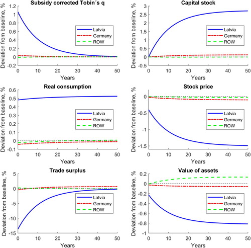
The time path of the capital stock in Figure 1 illustrates that a subsidy increases investments in the subsidized regions, and that this increase is largest at the beginning. Private capital stock accumulates above the initial benchmark level and converges to a new steady-state level (Figure 1, upper). If we had lower adjustment costs, we would observe an even stronger concentration of investments in the subsidized regions immediately after the shock.

Figure 1. Time paths of the key variables in the private investment subsidy scenario (with a local portfolio).

In the case of the lump-sum transfer, there is virtually no reaction on the capital market; prices are largely unaffected. However, household incomes rise in the supported regions, as do consumption and volume of savings. Additional assets are accumulated and the trade deficit is permanently larger (Figure 2).

Figure 2. Trade balance and consumption in the lump-sum transfer scenario.

An interesting observation is that under a global portfolio the subsidy effects for the supported regions are stronger than under a local portfolio (Table 1), to the tune of 14% on average. Why is this? Figure 1 (middle right) neatly reveals the mechanism. The subsidy causes the market value of installed private capital to decline. This drop matters in quantitative terms. It is important here to distinguish investment subsidies from subsidizing user costs of capital. The latter benefits all capital owners, both those owning the existing stock and those investing in new stocks. The former harms owners of existing stock, who then face new competition. While regional workers own the complementary factor, capital owners own a competing factor which becomes more abundant due to the lower cost of investment. Thus, households owning the local capital stock, which loses value due to the subsidy, will face a reduction in welfare gains. A further observation is that the welfare losses in the donor regions are lower in the case of global asset ownership.

The bottom part of Table 1 suggests that under global asset ownership the subsidy has a positive net effect on the EU as a whole. However, based on the sensitivity analysis employing alternative subsidy schemes, we find that this effect only holds true if the economic size of the regions supported is relatively small. For the subsidy under a local portfolio, the net effect on the EU is negative; for the transfer scenario, it is close to zero.

The rest of the world experiences negative welfare effects under the subsidy scenarios (which although small in relative terms are large in absolute terms, as Table 1 illustrates). The reason for this is the global relocation of investment towards the supported regions in the EU. The new investments in the rest of the world go down, there is a reduction in capital stock and output in comparison to the benchmark steady state. Temporarily, consumption decreases (in favour of investment in the EU) and the trade surplus increases (due to exports to the EU). Under a global portfolio, an additional negative effect in the rest of the world is the drop in value of capital stock owned in the supported regions. Overall, the subsidy leads to a cost in terms of global efficiency. In contrast, the transfer scenario is welfare-neutral for the rest of the world.

The impact of the diversity gains is demonstrated by including results from an alternative model set-up, in which the endogenous variety effect à la Dixit–Stiglitz is switched off. This is done by fixing product diversity of the supply of tradables in each region at their respective benchmark levels in equations (13)(13) $T_{rs}=\frac{S_r{\left(p_r^s{\mathrm{\Theta }}_{rs}\right)}^{-\sigma }{D}_s}{\sum _{r^{\mathrm{\prime }}}{S}_{r^{\mathrm{\prime }}}{\left(p_{r^{\mathrm{\prime }}}^s{\mathrm{\Theta }}_{r^{\mathrm{\prime }}s}\right)}^{-\sigma }},$(13) and (15)(15) $p_s^d=\psi {\left(\sum _r{S}_r{\left(p_r^s{\mathrm{\Theta }}_{rs}\right)}^{1-\sigma }\right)}^{1/\left(1-\sigma \right)},$(15) . The formulation then resembles a classical Armington (1969) assumption for trade in heterogeneous goods. Table C1 in Appendix C in the supplemental data online shows that in the subsidy scenarios the welfare gains for the supported regions shrink slightly. The diversity gains for the supported regions are thus visible, but they amount to only 0.2–0.6 per million in terms of the REV. Under a local portfolio, this small change makes households better off with a transfer than with a subsidy (thus, only weak effectiveness). For the donor regions, diversity gains seem to compensate a small part of the welfare costs of the subsidy. For the transfer scenario, the diversity gains play virtually no role at all.

The growth rate of capital and consumption in this alternative set-up without an endogenous variety effect is equal to the rate of Harrod neutral technical progress ($\xi$). Thus, in this case the homogeneity of model parameters across regions is not necessary for the saddle-path stability of model dynamics. We thus use this set-up to demonstrate that the main findings hold also under parameter heterogeneity.

Any parameter may be regarded as a candidate for regional heterogeneity, but tracing the entire parameter space in a robustness check is obviously impossible. For deep parameters such as the rates of depreciation or intertemporal subjective discounting the values are difficult to quantify even on national or global scale, and there is no indication if and to what extent they may vary across space. We thus follow the common practice to rely on a literature consensus in this regard, which does not allow for any reasonable regional differentiation and is widely accepted not only in growth modelling but also in standard cost–benefit analysis.

A sensible candidate for checking robustness is variation of parameters that might in principle be calibrated on a regional scale, if ideal accounting data were at hand. The one that may matter in the context of this paper is the share of tradables in final demand ($ϵ$), because spillovers of regional subsidies are suspected to work through a trade channel and may thus depend on the openness of regions to interregional trade. As we do not have the ideal regional accounting data at hand allowing to calibrate the parameter for all regions of the model, we vary it randomly in a robustness experiment, assuming it to be uniformly distributed in the range [0.55–0.65], instead of being 0.6 for all regions. This is a strong variation taking into account that, according to input–output data (Narayanan et al., 2012), the commodity composition of final demand is fairly uniform across countries and likely not much less uniform across regions.

Comparing Tables C1 and C2 in Appendix C in the supplemental data online with homogeneous and heterogeneous parameters, respectively, shows differences in detail as it should, given the fairly large parameter variation. Still, the differences are moderate, and there is no case where the qualitative conclusions regarding weak and strong effectiveness and the role of the portfolio composition are affected: the effects in columns (3)–(5) are ordered identically in Tables C1 and C2.

The final point here is the robustness of the modelling results with regard to alternative aggregation schemes. Table C3 online shows the results for aggregation 2 (with disaggregated regions in Bulgaria and Romania). We can now compare the results from different model runs. In the bottom part of Table 1 (columns 3–5), we report the sum over the absolute effects for the Polish regions. The values deviate only negligibly from the results for Poland as a single region in Table C3. The same is true of the disaggregated (Table C3) and aggregated (Table 1) versions for Bulgaria and Romania. The results for single-region countries (such as Latvia or Germany) and for the whole world are also virtually the same in both simulations. This demonstrates that the model is robust against different aggregation schemes.

Subsidy for public investment

Table 2 presents the welfare effects for the public investment subsidy scenarios and the corresponding transfer scenario. Again, the results are displayed for two extreme cases of private capital ownership (public capital is owned locally). Much as in the previous case, the results in Table 2 indicate that the subsidies for public investment produce positive welfare effects in the supported regions.

However, the results suggest that in terms of the size of the effects on the supported regions, the order of scenarios is different than in the case of the private investment subsidy described above. The supported regions gain most from the public investment subsidy under the local asset ownership scheme. The subsidy is strongly effective in this case, but the lump-sum transfer turns out to be only slightly inferior in terms of welfare impacts. Under the global asset portfolio, the gains for the subsidized regions are smallest (only weak effectiveness) and the EU as a whole suffers a substantial welfare loss.

The mechanism behind these results again has to do with the complementarity of production factors. When public capital is subsidized, it accumulates faster, which helps increase the productivity of other factors, including private capital. Under the global portfolio, these capital gains trickle down to other regions, while under the local portfolio they stay in the supported region. In contrast to the case of private investment subsidy, the market price of installed private capital in the supported region does not decline. After an initial leap it then converges to the steady-state level.

In terms of global efficiency, a public investment subsidy means that the welfare effects in the rest of the world are negative and the world as a whole is characterized by a welfare loss.

Further discussion

From the most fundamental perspective, simulated investment subsidies boost private and public capital accumulation in the subsidized regions. The supported regions invest more than they would otherwise, and the additional accumulated factor stock increases output and income in the supported regions, thus contributing to the goal of territorial development. This is consistent with the majority of recent econometric studies analysing European and national support schemes for lagging regions (e.g., de Castris & Pellegrini, 2012; Cerqua & Pellegrini, 2014; Percoco, 2017).

The results are also consistent with previous findings suggesting that the effects of regional policy depend on the economic conditions of the supported regions (Fratesi & Wishlade, 2017). In particular, trade openness has been previously shown to increase the effects of regional aid (Ederveen, Groot, & Nahuis, 2006). This correlation is included in our model through the modest diversity gains, which are higher if the costs of trade for the region are lower.

The welfare impacts of subsidies for public investment in our simulations remain close to the size of the EU funds, no major additional effects were discernible. A similar finding for the impact of EU funding in the period 2007–15 can be inferred from the results for selected regions reported by the recently published RHOMOLO model application (Di Comite et al., 2018). In this connection, it is worth noting that EU support for regional public infrastructure investment (which was allocated the largest budget in the period 2007–15) is not the key instrument advanced in the current debate about the future of EU Cohesion Policy. However, the calls for smart specialization (targeting specific types of activities in every region) and for an overall focus on supporting innovation, the knowledge economy and the development of human capital (Bachtler & Gorzelak, 2007) go far beyond the types of policy interventions that can be represented in the modelling framework of this paper.

As far as subsidies for private firms are concerned, current research and policy increasingly focus on the effects of research and development (R&D) subsidies (e.g., Montmartin & Massard, 2015; Garau & Lecca, 2015). Incorporating endogenous growth mechanisms into the multiregional modelling framework would allow simulation of the effects of innovation subsidies on long-term growth rates, which is a policy issue of high interest on which empirical findings are mixed. This direction would suggest itself as a natural extension of the modelling set-up presented here.

CONCLUSIONS

This paper uses a multiregional dynamic model to study the regional welfare impacts of investment subsidies for private and public capital. First, with regard to the methodology, it shows that a fully consistent multiregional neoclassical model with forward-looking agents can readily be implemented and solved, and that it is a useful tool both in policy analysis in general and in the study of investment subsidies in particular. We show that this model is robust to various regional aggregation settings, although the maximum number of regions is currently limited.

Second, we see that private investment subsidies are strongly effective. The supported regions enjoy welfare gains of similar magnitude to the EU funds allocated. The exact size of the welfare effects depends on the portfolio distribution held by the households. If households only own local stocks and are the only owners of those local stocks, part of the welfare gain is lost through the drop in share prices. This private capital devaluation effect of the investment subsidy has not been described in the literature so far. However, these interaction effects from the capital market are not very large, a finding that contrasts with some previous results reported from a static framework. Also, although the diversity gains generated by the model structure are small, they are still sufficient to make households in the supported regions better off under the subsidy than under lump-sum transfer.

Third, a subsidy for investment in public capital is at least weakly effective in the supported regions. The highest welfare gains are achieved under local asset ownership because in this case the productivity effects of public capital accumulation do not spill over to other regions. Effects on the supported regions under global asset ownership are however smaller than the effects from a lump-sum transfer. The divergent findings about the effectiveness of public and private investment subsidies under different capital ownership assumptions are one of the contributions made by this paper.

Finally, from the point of view of total welfare, investment subsidies are not efficient in all scenarios. We show that subsidies can lead to a welfare loss for the EU as a whole and that they definitely lead to welfare losses in the rest of the world, from which investments flow to the supported EU regions. The inefficiency is higher in the setting without diversity effects.

The results of the simulations in this paper are subject to several caveats. With this highly stylized model, we are naturally unable to provide a fully realistic impact assessment of EU regional policy. The simulation results are thus only an illustration of the regional welfare impacts under conditions of capital mobility and different asset ownership schemes. The key findings with respect to effectiveness in the target regions and overall inefficiency of investment subsidies, however, turn out to be robust against the chosen regional disaggregation and against slight model modifications, including certain parameter heterogeneity. Also, as this is a model with only one type of household per region, within-region redistribution effects of regional policy were not analysed. The only role of region-specific taxes that figures in the model is that of financing local (non-EU) public investment. Other aspects of regional tax systems are not considered.

ACKNOWLEDGEMENTS

An earlier version of this paper was published as TU Dresden CEPIE Working Paper No. 02/18 (http://nbn-resolving.de/urn:nbn:de:bsz:14-qucosa-235416). The authors are grateful to d’Artis Kancs for sharing with them the DG Regio data on regional subsidies; and to Claudia Baranzelli and Olga Ivanova for comments made on an earlier draft of this paper. Henning Meier provided excellent research support. The authors acknowledge the valuable input of the three anonymous referees that helped to improve this paper.

DISCLOSURE STATEMENT

No potential conflict of interest was reported by the authors.

REFERENCES

- Abel, A., & Blanchard, O. J. (1986). The present value of profits and cyclical movement in investment. Econometrica, 54, 249–273. doi: 10.2307/1913150
- Armington, P. S. (1969). A theory of demand for products distinguished by place of production. International Monetary Staff Papers, 16, 159–176. doi: 10.2307/3866403
- Bachtler, J., & Gorzelak, G. (2007). Reforming EU Cohesion Policy: A reappraisal of the performance of the structural funds. Policy Studies, 28(4), 309–326. doi: 10.1080/01442870701640682
- Baldwin, R., Forslid, R., Martin, P., Ottaviano, G., & Robert-Nicoud, F. (2003). Economic geography and public policy. Princeton: Princeton University Press.
- Barro, R., & Sala-i-Martin, X. (1995). Economic growth. New York: McGraw-Hill.
- Brandsma, A., Kancs, d., Monfort, P., & Rillaers, A. (2015). RHOMOLO: A dynamic spatial general equilibrium model for assessing the impact of Cohesion Policy. Papers in Regional Science, 94, S197–S221. doi: 10.1111/pirs.12162
- Bröcker, J. (1998). How would an EU-membership of the Visegrád countries affect Europe’s economic geography? Annals of Regional Science, 32, 91–114. Erratum (2000), 34, 469–471. doi: 10.1007/s001680050064
- Bröcker, J., & Korzhenevych, A. (2013). Forward looking dynamics in spatial CGE modelling. Economic Modelling, 31, 389–400. doi: 10.1016/j.econmod.2012.11.031
- Bröcker, J., Korzhenevych, A., & Schürmann, C. (2010). Assessing spatial equity and efficiency impacts of transport infrastructure projects. Transportation Research Part B, 44, 795–811. doi: 10.1016/j.trb.2009.12.008
- Cerqua, A., & Pellegrini, G. (2014). Do subsidies to private capital boost firms’ growth? A multiple regression discontinuity design approach. Journal of Public Economics, 109, 114–126. doi: 10.1016/j.jpubeco.2013.11.005
- Dall’erba, S., & Le Gallo, J. (2008). Regional convergence and the impact of European structural funds over 1989–1999: A spatial econometric analysis. Papers in Regional Science, 87(2), 219–244. doi: 10.1111/j.1435-5957.2008.00184.x
- de Castris, M., & Pellegrini, G. (2012). Evaluation of spatial effects of capital subsidies in the South of Italy. Regional Studies, 46(4), 525–538. doi: 10.1080/00343404.2010.509130
- Di Comite, F., Lecca, P., Monfort, P., Persyn, D., & Piculescu, V. (2018). The impact of Cohesion Policy 2007–2015 in EU regions: Simulations with the RHOMOLO Interregional Dynamic General Equilibrium Model (Technical Report No. 03/2018). Seville: Joint Research Centre (JRC), European Commission.
- Dupont, V., & Martin, P. (2006). Subsidies to poor regions and inequalities: Some unpleasant arithmetic. Journal of Economic Geography, 6, 223–240. doi: 10.1093/jeg/lbi019
- Ederveen, S., Groot, H. L., & Nahuis, R. (2006). Fertile soil for structural funds? A panel data analysis of the conditional effectiveness of European Cohesion Policy. Kyklos, 59(1), 17–42. doi: 10.1111/j.1467-6435.2006.00318.x
- European Union. (2017). My region, my Europe, our future: Seventh report on economic, social and territorial cohesion. Luxembourg: Publications Office of the European Union.
- Eurostat. (2017). Regional economic accounts. Retrieved from http://ec.europa.eu/eurostat/ web/regions/data/database
- Fratesi, U. (2016). Impact assessment of EU Cohesion Policy: Theoretical and empirical issues. In S. Piattoni, & L. Polverari (Eds.), Handbook on Cohesion Policy in the EU (pp. 443–460). Cheltenham: Edward Elgar.
- Fratesi, U., & Wishlade, F. G. (2017). The impact of European Cohesion Policy in different contexts. Regional Studies, 51(6), 817–821. doi: 10.1080/00343404.2017.1326673
- Fuest, C., & Huber, B. (2000). Why do governments subsidise investment and not employment? Journal of Public Economics, 78(1–2), 171–192. doi: 10.1016/S0047-2727(99)00115-2
- Garau, G., & Lecca, P. (2015). The impact of regional R&D subsidy in a computable general equilibrium model. International Regional Science Review, 38(4), 319–357. doi: 10.1177/0160017613485758
- Huggins, R. (1998). An evaluation of European Union Objective 2 Programmes in industrial South Wales 1989–93. European Urban and Regional Studies, 5(4), 291–303. doi: 10.1177/096977649800500401
- Hummels, D. (1999). Toward a geography of trade costs (Manuscript). University of Chicago.
- Lolos, S. E. G. (1998). Success and failure of economic policies: The experience of Greece and Portugal. Comparative Economic Studies, 40(1), 72–102. doi: 10.1057/ces.1998.4
- Montmartin, B., & Massard, N. (2015). Is financial support for private R&D always justified? A discussion based on the literature on growth. Journal of Economic Surveys, 29(3), 479–505. doi: 10.1111/joes.12067
- Narayanan, B., Aguiar, A., & McDougall, R. (2012). Global trade, assistance, and production: The GTAP 8 data base. Center for Global Trade Analysis, Purdue University. Retrieved from http://www.gtap.agecon.purdue.edu/databases/v8/
- OpenStreetMap. (2017). Planet dump. Retrieved from https://planet.osm.org. https://www.openstreetmap.org
- Percoco, M. (2017). Impact of European Cohesion Policy on regional growth: Does local economic structure matter? Regional Studies, 51(6), 833–843. doi: 10.1080/00343404.2016.1213382
- Piattoni, S., & Polverari, L. (Eds.). (2016). Handbook on Cohesion Policy in the EU. Cheltenham: Edward Elgar.
- Ribeiro, L. C. D. S., Domingues, E. P., Perobelli, F. S., & Hewings, G. J. D. (2018). Structuring investment and regional inequalities in the Brazilian Northeast. Regional Studies, 52(5), 727–739. doi: 10.1080/00343404.2017.1327709
- United Nations Statistics Division. (2017a). International trade statistics database. Retrieved from https://comtrade.un.org/
- United Nations Statistics Division. (2017b). National accounts main aggregates database. Retrieved from https://unstats.un.org/unsd/snaama/selbasicFast.asp
- Varga, A. (2017). Place-based, spatially blind, or both? Challenges in estimating the impacts of modern development policies: The case of the GMR policy impact modeling approach. International Regional Science Review, 40(1), 12–37. doi: 10.1177/0160017615571587