The impact of regional inequality on economic growth: a spatial econometric approach

ABSTRACT

This paper investigates the relationship between economic growth and regional income inequality in a spatial econometric perspective. The role of space in the measure of inequality is discussed, and a new theoretical model that relates inequality with economic growth is introduced. The proposed model extends a spatial Mankiw–Romer–Weil specification by introducing regional income inequality as a determinant of economic growth. The measure of inequality proposed as a covariate in the model is derived by a spatial decomposition of the Gini index. An empirical analysis focused on European Union NUTS-2 regions is carried out to illustrate the model.

KEYWORDS:

• regional disparities
• economic convergence
• spatial analysis
• European Union NUTS-2 regions

JEL:

• C31
• D63
• O47
• O52

INTRODUCTION

There is a body of literature examining the relationship between inequality and economic growth. Using individual income data, the impact of inequality on growth performances has been mainly investigated through cross-sectional growth regressions, where the average growth rate of income per capita is regressed on initial inequality and several other control variables (Alesina & Rodrik, 1994; Persson & Tabellini, 1994). Using cross-section analysis, Chen (2003) assessed the existence of an inverted ‘U’-shaped relationship between initial income distribution and long-run economic growth. Using panel data, Li and Zou (1998) and Forbes (2000) proposed fixed-effects estimates. Fixed-effects and generalized method of moments (GMM) estimations of the relationship between inequality and growth have been performed by Panizza (2002). An attempt to separate long- and short-run influences of inequality on growth has been made by Partridge (2005).

Depending on the data and the methodologies used, the empirical literature reported conflicting results about the effects of inequality on economic growth. A negative impact of inequality on growth has been mainly supported by empirical cross-country studies (Alesina & Rodrik, 1994; Persson & Tabellini, 1994), while several other studies derived a positive relationship (Forbes, 2000; Li & Zou, 1998). Panizza (2002) found a negative relationship between inequality and growth, which, however, is not robust to small changes in data or econometric specifications.

A different approach has been proposed in some contributions focused on regional disparities, their determinants, and their relations with growth and the level of economic development (Lessmann, 2014; Lessmann & Seidel, 2017; Petrakos et al., 2005). Furthermore, the inequality in the distribution of economic activities has been linked to both geographical characteristics and variables related to the level of development by Henderson et al. (2018).

The need to assess the impact of inequality on growth in a spatial perspective has been highlighted in the recent literature (Martino & Perugini, 2008; Rey & Janikas, 2005). Along this research line, Janikas and Rey (2008) proposed a spatial analysis that allows for simultaneous interactions between regional growth and inequality. A spatially augmented model which allows intra-regional disparities to be one of the determinants of regional economic growth has been proposed by De Dominicis (2014).

Following these contributions, in this paper we introduce a new theoretical growth model that relates economic growth with regional inequality in a spatial perspective. Based on the spatially augmented Mankiw–Romer–Weil (MRW) (Mankiw et al., 1992) model introduced by Fischer (2011), the proposed specification allows the impact of regional inequality on the growth process to be assessed. The model includes a regional inequality measure as a covariate. This measure is derived by the spatial decomposition of the Gini index introduced by Rey and Smith (2013). In addition to verifying the impact of inequality on growth in a regional economy, the proposed model allows the extent to which regional growth is influenced by inequality in neighbouring regions to be assessed.

Our approach is different in some important aspects from De Dominicis (2014), who also investigated this issue. First, while the theoretical model developed by De Dominicis is based on the specification given in Ertur and Koch (2007), our model extends the framework proposed by Fischer (2011).

Besides, our approach defines a theoretical model where the impact of human capital on growth is explicitly considered. Conversely, in De Dominicis (2014), the impact of human capital is only empirically estimated without any theoretical implication. For this reason, our theoretical model can be considered as a methodological extension of the De Dominicis approach.

Finally, while De Dominicis (2014) considered the within component of the Theil index (Theil, 1967) as a measure of regional inequality, we use the within component of the Gini index and its spatial decomposition proposed by Rey and Smith (2013). Specifically, we introduce as an inequality variable in our model the non-spatial component of the within-region inequality, which expresses the component of intra-regional inequality that is not influenced by the spatial interactions among regional units. This definition allows us to consider the idiosyncratic component of inequality, isolating the spatial component of intra-regional inequality whose impact could alter the real effect of inequality on regional growth.

The proposed model is illustrated through an empirical analysis focused on European Union (EU) NUTS-2 regions over the period 2003–16. EU regions represent interesting units of analysis. In fact, the persistence of inequalities across EU regions, exacerbated by the global financial crisis, requires the definition of regional policies aimed at enhancing growth and regional equity. Most of the EU funds and programmes are specifically delivered for less developed regions to promote the convergence of these regions toward the richer ones. Considering the relationship between inequality and growth facilitates the assessment of the role that disparities within regional economies play in the convergence process. Within-region disparities could thus become a variable on which regional policies could be targeted to promote growth and convergence. The introduction of spatial effects in the analysis entails considering both spatial similarities and instabilities across space, facilitating a study of disparities and reduction policies more anchored to the characteristics of the spatial units under consideration.

Accounting for the peculiarities of regional economies could offer useful insights into the major socioeconomic trends that have interested the EU in recent decades. In fact, the higher internal disparities characterizing the new accession member states could impact on their catch-up process toward more developed regional economies. Assessing such dynamics also offers useful indications to address policies targeted to different regional contexts.

The rest of the paper is organized as follows. Next, we discuss the general theoretical growth model and our specification. We then present an empirical application concerning European NUTS-2 regions. Finally, we provide some concluding remarks and future research agenda.

A THEORETICAL MODEL OF ECONOMIC GROWTH

Analysing the relationship between regional inequality and economic growth in a spatial perspective requires an appropriate model specification. In fact, regional growth could be influenced by inequality within the regional economy as well as by inequality in neighbouring regions. This spatial dependence effect is so included in the proposed model that we derive theoretically.

Our model specification is obtained as an extension of the spatial MRW model developed by Fischer (2011). However, while Fischer considers as the dependent variable in the model the level of regional gross domestic product (GDP) at the end of the period, we focus on the GDP growth rate, testing for the $\text{β}$-convergence hypothesis.

In our proposal, the spatially augmented MRW is modified by introducing a measure of regional inequality among the covariates. Specifically, as in De Dominicis (2014), in our model the investment in physical capital is expressed as a function of inequality. This assumption allows the impact of inequality on growth to be assessed, and is based upon the idea that higher inequality among regions stimulates higher investments from richer regions. Moreover, according to standard economic theories, saving and investment are assumed to be identical and is a fairly typical result that the redistribution of resources from rich to poor tends to lower the aggregate rate of saving in an economy (Thorbecke & Charumilind, 2002). This argument found support in Kaldor (1956) who highlighted that a high initial inequality of income favours high saving, because of the higher propensity to save that rich people have with respect to poor people and, thus, it stimulates higher capital accumulation. On the same line, Galor (2000) argues that high income inequality has a positive impact on savings, resulting in a higher physical capital accumulation. Furthermore, a positive relationship between inequality and aggregate saving has been recently reported by Koo and Song (2016) who found a greater and statistically more significant effect for richer and more developed countries.

In this paper we assume that each regional economy is characterized by a Cobb–Douglas production function that, for region $i$ at time $t$, is specified as follows: (1) $Y_{it}=A_{it}{C}_{it}^{{\alpha }_C}{H}_{it}^{{\alpha }_H}{L}_{it}^{1-{\alpha }_C-{\alpha }_H}$(1) where $Y$ is the output; $A$ is the level of technology; $C$ is the physical capital; $H$ is the human capital; and $L$ is the labour. The exponents ${\alpha }_C$ and ${\alpha }_H$ are the output elasticities with respect to physical capital and human capital, respectively. These output elasticities are positive constants (i.e., ${\alpha }_C,{\alpha }_H>0$) such that ${\alpha }_C+{\alpha }_H<1$, hence the production function has decreasing returns to both types of capital.

Denoted by $s_i^C$ and $s_i^H$, which are the fractions of output $Y_{it}$ invested in physical capital and human capital, respectively; and by $\delta$, which is a rate of depreciation that is assumed to be constant and identical for both physical and human capital, the dynamic equations for $C$ and $H$ are given by: (2) ${\dot{C}}_{it}=s_i^C{Y}_{it}-\delta C_{it}$(2) (3) ${\dot{H}}_{it}=s_i^H{Y}_{it}-\delta H_{it}$(3) where the dots over the variables indicate their time-derivatives. The dynamic equation for labour and technology are ${\dot{L}}_{it}=n_i{L}_{it}$ and ${\dot{A}}_{it}=g{A}_{it}$, where $n_i$ is the working population growth rate; and $g$ is a constant growth rate for technology. Now define the per worker quantities for output, physical capital and human capital as $y_{it}=Y_{it}/L_{it}$, $c_{it}=C_{it}/L_{it}$ and $h_{it}=H_{it}/L_{it}$, respectively. The production function (1) in per worker terms becomes: (4) $y_{it}=A_{it}{c}_{it}^{{\alpha }_C}{h}_{it}^{{\alpha }_H}$(4) Introducing spatial externalities, the level of technology, for each region $i$, is expressed as follows: (5) $A_{it}={\mathrm{\Omega }}_t{c}_{it}^{{\varphi }_C}{h}_{it}^{{\varphi }_H}\prod _{j=1}^n{A}_{jt}^{\gamma w_{ij}}$(5) According to equation (5), the function $A_{it}$ depends on four terms. The first term, ${\mathrm{\Omega }}_t$, represents the proportion of technological progress that, by assumption, is exogenous and identical for all regions. It is defined by ${\mathrm{\Omega }}_t={\mathrm{\Omega }}_0{e}^{\tau }$, where $\tau$ is the exogenous technological progress growth rate; and ${\mathrm{\Omega }}_0$ is its initial level. The next two terms imply that the level of technology for each region $i$ depends on both the level of physical capital per worker, $c_{it}$, and the level of human capital per worker, $h_{it}$. This implies that investments in both physical and human capital increase not only capital stocks but also the level of technology through knowledge spillovers. The strength of these externalities is determined by the parameters ${\varphi }_C$, with $0\le {\varphi }_C<1$, and ${\varphi }_H$, with $0\le {\varphi }_H<1$, respectively. The last term implies that the level of technology of region i also depends on the level of technology of its neighbour regions $j$, for$j=1,2,\dots ,N$. The degree of technological interdependence among regions depends on the scalar parameter $\gamma$, with $0\le \gamma <1$, and on the proximity between regions that is summarized by the matrix $W$. The $\left(i,j\right)$-th element of $W$, $w_{ij}$, is such that $0\le w_{ij}\le 1$, with $w_{ij}=0$ for $i=j$, and ${\sum }_{j=1}^N{w}_{ij}=1$. For regions that are neighbours of region $i$, $w_{ij}>0$, for $i,j=1,2,\dots ,N$.

The dynamic equations for physical capital per worker and human capital per worker (equations 2 and 3) become: (6) ${\dot{c}}_{it}=s_i^C{y}_{it}-(\delta +n_i)c_{it}$(6) (7) ${\dot{h}}_{it}=s_i^H{y}_{it}-(\delta +n_i)h_{it}$(7) Besides, we assume that the fraction of output that is invested in physical capital is a function of a measure of inequality, that is, $s_i^C=f\left(G_i\right)=Ine{q}_i$, where $G_i$ is a measure of inequality for region $i$. This assumption implies that higher inequality among regions should stimulate higher investments from richer regions.

Following this assumption, equation (6) can be rewritten as: (8) ${\dot{c}}_{it}=Ine{q}_i{y}_{it}-(\delta +n_i)c_{it}$(8) Equations (8) and (7) imply that the physical capital output and human capital output are constant so that: (9) ${\displaystyle \frac{c_i^{\ast }}{y_i^{\ast }}={\displaystyle \frac{Ine{q}_i}{\left(\delta +g+n_i\right)}}}$(9) (10) ${\displaystyle \frac{h_i^{\ast }}{y_i^{\ast }}={\displaystyle \frac{s_i^H}{\left(\delta +g+n_i\right)}}}$(10) where the asterisk denotes the steady-state value of the variable. The steady-state conditions for the physical capital and human capital variables can be derived by equations (9) and (10), respectively. Substituting these expressions in equation (4) and taking the logarithm, after some algebra, we obtain: (11) $\begin{array}{rl}\mathrm{l}\mathrm{n}{y}_i^{\ast }=& {\displaystyle \frac{1}{1-\eta }\mathrm{l}\mathrm{n}{\mathrm{\Omega }}_t+{\displaystyle \frac{{\alpha }_C+{\varphi }_C}{1-\eta }\mathrm{l}\mathrm{n}Ine{q}_i+{\displaystyle \frac{{\alpha }_H+{\varphi }_H}{1-\eta }\mathrm{l}\mathrm{n}{s}_i^H}}}\\ & -{\displaystyle \frac{\eta }{1-\eta }\mathrm{l}\mathrm{n}\left(\delta +g+n_i\right)-{\displaystyle \frac{{\alpha }_C}{1-\eta }\gamma \sum _{j=1}^N{w}_{ij}\mathrm{l}\mathrm{n}Ine{q}_i}}\\ & -{\displaystyle \frac{{\alpha }_H}{1-\eta }\gamma \sum _{j=1}^N{w}_{ij}\mathrm{l}\mathrm{n}{s}_j^H+{\displaystyle \frac{{\alpha }_C+{\alpha }_H}{1-\eta }\gamma }}\\ & \sum _{j=1}^N{w}_{ij}\ln \left(\delta +g+n_j\right)+{\displaystyle \frac{1-{\alpha }_C-{\alpha }_H}{1-\eta }\gamma \sum _{j=1}^N{w}_{ij}\mathrm{l}\mathrm{n}{y}_j^{\ast }}\end{array}$(11) where $\eta ={\alpha }_C+{\alpha }_H+{\varphi }_C+{\varphi }_H$. In order to define the convergence of output per worker in a given region to the region’s steady-state value, we consider a log-linearization of equations (8) and (7) around steady states, which lead to a system of linear differential equations that can be solved by using the technique developed by Ertur and Koch (2007). Postulating that the gap of region i relative to its own steady state is proportional to the corresponding gap for region j, it follows that: (12) ${\displaystyle \frac{d\mathrm{l}\mathrm{n}{y}_{it}}{dt}=g-{\lambda }_i\left[\mathrm{l}\mathrm{n}{y}_{it}-\mathrm{l}\mathrm{n}{y}_i^{\ast }\right]}$(12) where $g$ denotes the constant growth rate of physical and human capital; and ${\lambda }_i$ is the speed of convergence. Solving equation (12) for $\mathrm{l}\mathrm{n}{y}_{it}$, and subtracting from both sides the output per worker at some initial date, $\mathrm{l}\mathrm{n}{y}_{i0}$, we obtain the following expression, written in a matrix notation: (13) $G=gt\iota -D{y}_0+D{y}^{\mathbf{\ast }}$(13) where $G=y_t-y_0$, with $y_t$ the $N\times 1$ vector of logarithms of output per worker at time $t$; and $y_0$ the $N\times 1$ vector of logarithms of the initial level of output per worker, $\iota$ is a $N\times 1$ vector of ones, $D$ is a $N\times N$ diagonal matrix with ($1-e^{{\lambda }_{i}t}$) elements on the main diagonal, and $y^{\mathbf{\ast }}$ is the $N\times 1$ vector of logarithms of output per worker at steady state. Following the rationale of Ertur and Koch (2007), rewriting equation (11) in a matrix notation we have: (14) $\begin{array}{r}{y}^{\mathbf{\ast }}=(I-\rho W{)}^{-1}[{\displaystyle \frac{1}{1-\eta }\mathrm{\Omega }+{\displaystyle \frac{{\alpha }_C+{\varphi }_C}{1-\eta }In+{\displaystyle \frac{{\alpha }_H+{\varphi }_H}{1-\eta }S}}}\\ & -{\displaystyle \frac{{\alpha }_C\gamma }{1-\eta }WIn-{\displaystyle \frac{{\alpha }_H\gamma }{1-\eta }WS]}}\end{array}$(14) where $\rho ={\displaystyle \frac{\gamma \left(1-{\alpha }_C-{\alpha }_H\right)}{1-\eta }}$, $In$ and $S$ are the $N\times 1$ vectors of the logarithms of inequality measures and saving rates of human capital (i.e., $\mathrm{l}\mathrm{n}{s}_i^H$), respectively, divided by the effective rate of depreciation (i.e., by $\mathrm{l}\mathrm{n}\left(\delta +g+n_i\right)$). Substituting (14) in (13), and pre-multiplying both sides by the inverse of $D(I-\rho W{)}^{-1}$, after rearranging terms, we obtain: (15) $\begin{array}{rl}G& =gt\iota -\rho gtDW{D}^{-1}\iota +{\displaystyle \frac{1}{1-\eta }D\mathrm{\Omega }}\\ & -D{y}_0+{\displaystyle \frac{{\alpha }_C+{\varphi }_C}{1-\eta }DIn+{\displaystyle \frac{{\alpha }_H+{\varphi }_H}{1-\eta }DS+\rho DW{y}_0}}\\ & -{\displaystyle \frac{{\alpha }_C\gamma }{1-\eta }DWIn-{\displaystyle \frac{{\alpha }_H\gamma }{1-\eta }DWS-\rho DW{D}^{-1}G}}\end{array}$(15) Equation (15) can be rewritten for region $i$ as follows: (16) $\begin{array}{rl}\mathrm{l}\mathrm{n}{y}_{it}-& \mathrm{l}\mathrm{n}{y}_{i0}={\mathrm{\Delta }}_i-\left(1-e^{{\lambda }_{i}t}\right)\mathrm{l}\mathrm{n}{y}_{i0}+\left(1-e^{{\lambda }_{i}t}\right){\displaystyle \frac{{\alpha }_C+{\varphi }_C}{1-\eta }\mathrm{l}\mathrm{n}Ine{q}_i}\\ +& \left(1-e^{{\lambda }_{i}t}\right){\displaystyle \frac{{\alpha }_H+{\varphi }_H}{1-\eta }\mathrm{l}\mathrm{n}{s}_i^H-\left(1-e^{{\lambda }_{i}t}\right){\displaystyle \frac{\eta }{1-\eta }\mathrm{l}\mathrm{n}\left(\delta +g+n_i\right)}}\\ +& \left(1-e^{{\lambda }_{i}t}\right){\displaystyle \frac{1-{\alpha }_C-{\alpha }_H}{1-\eta }\gamma \sum _{j=1}^N{w}_{ij}\mathrm{l}\mathrm{n}{y}_{j0}}\\ & -\left(1-e^{{\lambda }_{i}t}\right){\displaystyle \frac{{\alpha }_C}{1-\eta }\gamma \sum _{j=1}^N{w}_{ij}\mathrm{l}\mathrm{n}Ine{q}_j}\\ & -\left(1-e^{{\lambda }_{i}t}\right){\displaystyle \frac{{\alpha }_H}{1-\eta }\gamma \sum _{j=1}^N{w}_{ij}\mathrm{l}\mathrm{n}{s}_j^H+\left(1-e^{{\lambda }_{i}t}\right){\displaystyle \frac{{\alpha }_C+{\alpha }_H}{1-\eta }\gamma \sum _{j=1}^N{w}_{ij}\ln \left(\delta +g+n_j\right)}}\\ & +\left(1-e^{{\lambda }_{i}t}\right){\displaystyle \frac{1-{\alpha }_C-{\alpha }_H}{1-\eta }\gamma \sum _{j=1}^N{\displaystyle \frac{1}{1-e^{{\lambda }_{i}t}}{w}_{ij}\left(\mathrm{l}\mathrm{n}{y}_{it}-\mathrm{l}\mathrm{n}{y}_{i0}\right)}}\end{array}$(16) where: ${\mathrm{\Delta }}_i=gt-\rho gt\left(1-e^{{\lambda }_{i}t}\right)\sum _{j=1}^N{\displaystyle \frac{w_{ij}}{1-e^{{\lambda }_{j}t}}+{\displaystyle \frac{1-e^{{\lambda }_{i}t}}{1-\eta }\mathrm{l}\mathrm{n}{\mathrm{\Omega }}_t.}}$Equation (16) states that the growth rate of output per worker, in region $i,$ depends negatively on its initial level, positively on inequality and on human capital investment rate, and negatively on the population growth rate. The growth rate of output per worker in region $i$ also depends on the same variables in the neighbouring regions $j,$ identified by $w_{ij}>0$, because of technological interdependence (Ertur & Koch, 2007). Specifically, it is negatively influenced by inequality and human capital investment rate in neighbouring regions and is positively influenced by their working population growth rate. As a further evidence in equation (16), the initial level of output per worker in neighbouring regions has a positive influence on the growth rate of output per worker in region i. Finally, the last term in equation (16) represents the rate of growth of output per worker in the neighbour regions and reflects the spatial autocorrelation process that is implied by the technological interdependence.

MODEL SPECIFICATION

The inequality variable

Our approach represents an extension of the spatial MRW introduced by Fischer (2011), where an inequality measure is included among the explanatory variables. In our model specification the inequality variable expresses the intra-regional inequality, that is, the level of internal inequality characterizing each regional unit.

Specifically, in our proposal we define and use an inequality index that is based on the non-spatial component of the within-region Gini index.

The Gini index $G$ can be decomposed in three terms, such as the within-region inequality $G_{\mathrm{w}\mathrm{i}\mathrm{t}\mathrm{h}\mathrm{i}\mathrm{n}}$, the between-region inequality $G_{\mathrm{b}\mathrm{e}\mathrm{t}\mathrm{w}\mathrm{e}\mathrm{e}\mathrm{n}}$, and a residual or interaction term $R$ (Mookherjee & Shorrocks, 1982; Shorrocks & Wan, 2005). While the between-group component captures the interregional inequality, and thus measures the distance between the average GDP of each region, the within-group term expresses the distance between the GDP values observed for spatial units that belong to the same region. The latter component thus expresses the inequality in each regional economy and could be assumed as influencing the economic growth rate in each region (see also De Dominicis, 2014).

Considering $N$ NUTS-2 regions labelled as $i=1,2,\dots ,N$ with respective mean income and population share ${\mu }_i$ and $p_i$, the within-term of the Gini index can be expressed as: (17) $G_{\mathrm{w}\mathrm{i}\mathrm{t}\mathrm{h}\mathrm{i}\mathrm{n}}=\sum _{i=1}^N{p}_i^2{\displaystyle \frac{{\mu }_i}{\mu }{G}_i}$(17) where $\mu$ represents the mean of the overall income distribution; and $G_i$ is the Gini index for region i. The index in (17) represents a kind of average of the inequality values within each regional unit, and is fully specified by information about population share, mean income and inequality values.

To compute the Gini index $G_i$ for each NUTS-2 region $i$, it is needed to consider the value of income $y_l$ of each $l$ NUTS-3 sub-region that belongs to the specific NUTS-2 region $i$, with$l=1,2,\dots ,M_i$ . The Gini index $G_i$ is thus defined as: (18) $G_i={\displaystyle \frac{{\sum }_{l=1}^{M_i}{\sum }_{z=1}^{M_i}\left|y_l-y_z\right|}{2M_i^2{\overline{y}}_i}}$(18) where: ${\overline{y}}_i={\sum }_{l=1}^{M_i}{y}_l/M_i.$

To define our measure of inequality, we apply the spatial decomposition of the Gini index into its neighbour and non-neighbour components introduced by Rey and Smith (2013). Other contributions in this direction have been proposed by Arbia (2001), Márquez et al. (2019) and Panzera and Postiglione (2020).

Denoted by $v_{lz}$, the generic element of the spatial weight matrix $\mathit{V}$, which summarizes the proximity between the spatial units at NUTS-3 level, the Gini index in (18) can be expressed as follows (Rey & Smith, 2013): (19) $G_i={\displaystyle \frac{{\sum }_{l=1}^{M_i}{\sum }_{z=1}^{M_i}{v}_{lz}\left|y_l-y_z\right|}{2M_i^2{\overline{y}}_i}+{\displaystyle \frac{{\sum }_{l=1}^{M_i}{\sum }_{z=1}^{M_i}(1-v_{lz})\left|y_l-y_z\right|}{2M_i^2{\overline{y}}_i}=N{G}_i+NN{G}_i}}$(19) where, for each NUTS-2 region $i$, the first term on the right-hand side represents the neighbour component ($N{G}_i$), and the second one represents the non-neighbour component ($NN{G}_i$). This decomposition reveals that the Gini index nests a measure of spatial autocorrelation. As the spatial autocorrelation increases, the $NN{G}_i$ component should grow relatively to the $N{G}_i$ component, since values similarity in space would be in effect. The result is the opposite in the presence of negative spatial autocorrelation, since the difference between the variate values observed for non-neighbour pairs would be smaller than that between neighbour pairs. In either case, the degree of spatial autocorrelation can be assessed by comparing the relative contribution of these two components (Rey & Smith, 2013). According to this interpretation, the $NN{G}_i$ component could be considered as the spatial component of $G_i$, which changes in the same direction as the positive spatial autocorrelation relationship. The non-spatial component of inequality can be thus identified and measured by the $N{G}_i$ component. The identification of the spatial and non-spatial components of inequality allows a better understanding of the phenomenon and can offer useful insights for assessing the impact of inequality on regional growth.

Equation (17) can be thus rewritten as: (20) $G_{\mathrm{w}\mathrm{i}\mathrm{t}\mathrm{h}\mathrm{i}\mathrm{n}}=\sum _{i=1}^N{p}_i^2{\displaystyle \frac{{\mu }_i}{\mu }N{G}_i+\sum _{i=1}^N{p}_i^2{\displaystyle \frac{{\mu }_i}{\mu }NN{G}_i=N{G}_{\mathrm{w}\mathrm{i}\mathrm{t}\mathrm{h}\mathrm{i}\mathrm{n}}+NN{G}_{\mathrm{w}\mathrm{i}\mathrm{t}\mathrm{h}\mathrm{i}\mathrm{n}}}}$(20) where $N{G}_i$ and $NN{G}_i$ indicate the neighbour and non-neighbour components, respectively, of the Gini index within region $i$, with $i=1,2,\dots ,N.$ In our model we consider, for each region $i$, the non-spatial inequality ($Ine{q}_i=p_i^2{\displaystyle \frac{{\mu }_i}{\mu }N{G}_i}$, the summands of the first term on the right side of equation 20). Since population-weighted inequality indices are considered, instead of assuming the GDP per worker as representative of the whole region, we account for how many individuals this GDP per worker represents (Mookherjee & Shorrocks, 1982). Hence, weighting by population facilitates accounting for regional sizes that, especially in the European context, present relevant differences (Portnov & Felsenstein, 2010). This approach also appears consistent with the approach proposed by De Dominicis (2014), which quantifies intra-regional inequality in the EU using the within component of the Theil index that implicitly includes the weighting by population.

The non-neighbour component introduced in the model represents the component of inequality that is not influenced by spatial autocorrelation in the GDP values. However, the spatial interactions among regional economies are included in the model by considering the spatial lag of the inequality variable.

The empirical model

Assuming parameter homogeneity (${\lambda }_i=\lambda$ for all $i$), the empirical counterpart of the model given in equation (16) can be expressed, at a given time, for region $i$, as follows: (21) $\begin{array}{rl}{g}_i& ={\text{β}}_0+{\text{β}}_1\mathrm{l}\mathrm{n}{y}_{i0}+{\text{β}}_2\mathrm{l}\mathrm{n}Ine{q}_{i0}+{\text{β}}_3\mathrm{l}\mathrm{n}{s}_i^H\\ & +{\text{β}}_4\ln \left(\delta +g+n_i\right)+\rho \sum _{j=1}^N{w}_{ij}{g}_j+{\rho }_1\sum _{j=1}^N{w}_{ij}\mathrm{l}\mathrm{n}{y}_{j0}\\ & +{\rho }_2\sum _{j=1}^N{w}_{ij}\mathrm{l}\mathrm{n}Ine{q}_i+{\rho }_3\sum _{j=1}^N{w}_{ij}\mathrm{l}\mathrm{n}{s}_i^H\\ & +{\rho }_4\sum _{j=1}^N{w}_{ij}\ln \left(\delta +g+n_j\right)+{ϵ}_i\end{array}$(21) where: $g_i={\displaystyle \frac{1}{T}\mathrm{l}\mathrm{n}\left({\displaystyle \frac{y_{it}}{y_{i0}}}\right)}$with $T$ denotes the number of time periods under investigation; $y_{it}$ and $y_{i0}$ express the GDP values per worker at the final and initial periods, respectively; and the inequality variable is expressed as: $\mathrm{l}\mathrm{n}Ine{q}_{i0}=\mathrm{l}\mathrm{n}\left(p_{i0}^2{\displaystyle \frac{{\mu }_{i0}}{{\mu }_0}N{G}_{i0}}\right),$where the subscript indicates, for all the quantities, that they refer to the initial time period. Considering the initial level of inequality is in line with the specification proposed by De Dominicis (2014), and also appears consistent with the assumption about the relation between initial inequality and investments on which the theoretical model is based (Galor, 2000; Kaldor, 1956; Koo & Song, 2016).

The parameter ${\text{β}}_0$ is a constant: ${ϵ}_i\sim N\left(0,{\sigma }^2\right),$as are the error terms: ${\text{β}}_1=-{\displaystyle \frac{1-e^{-\lambda T}}{T}}$ ${\text{β}}_2=-{\displaystyle \frac{1-e^{-\lambda T}}{T}{\displaystyle \frac{{\alpha }_C+{\varphi }_C}{1-\eta }}}$ ${\text{β}}_3=-{\displaystyle \frac{1-e^{-\lambda T}}{T}{\displaystyle \frac{{\alpha }_H+{\varphi }_H}{1-\eta },{\text{β}}_4=-{\displaystyle \frac{1-e^{-\lambda T}}{T}{\displaystyle \frac{\eta }{1-\eta },{\rho }_1={\displaystyle \frac{1-e^{-\lambda T}}{T}{\displaystyle \frac{\left(1-{\alpha }_C-{\alpha }_H\right)}{1-\eta }\gamma }}}}}}$ $\begin{array}{rl}& {\rho }_2={\displaystyle \frac{1-e^{-\lambda T}}{T}{\displaystyle \frac{{\alpha }_C}{1-\eta }\gamma ,{\rho }_3={\displaystyle \frac{1-e^{-\lambda T}}{T}{\displaystyle \frac{{\alpha }_H}{1-\eta }\gamma ,}}}}\\ & {\rho }_4={\displaystyle \frac{1-e^{-\lambda T}}{T}{\displaystyle \frac{{\alpha }_{C+}{\alpha }_H}{1-\eta }\gamma }}\end{array}$

and $\rho ={\displaystyle \frac{\gamma \left(1-{\alpha }_C-{\alpha }_H\right)}{1-\eta }.}$

The specification in (21) is known in literature as the spatial Durbin model (SDM) (LeSage & Pace, 2009). The SDM introduces a spatial lag on the dependent variable as well as on all the explanatory variables.

The linear specification in (21) is supported by the theoretical model proposed and developed in the previous section. When the empirical specifications are not supported by the theory, the unknown functional form represents a potential source of misspecification. This issue could be addressed by adopting a semiparametric framework, which is generally more flexible with respect to parametrical models. Semiparametric specifications that combine non-linearity with the simultaneous treatment of spatial dependence and spatial heterogeneity have been proposed in the recent literature (Basile & Gress, 2005; McMillen, 2012). A penalized-spline SDM has been introduced by Basile et al. (2014). This model represents an important tool to identify the functional form of the relationship between the response variable and its predictors, and even in the presence of structured model can be useful to distinguish between substantive spatial dependence (i.e., spatial spillovers) and spatial dependence generated by omitted variables.

The substantive spatial dependence occurs when the variable of interest at one location is influenced by its values at other locations and is captured by spatial weight matrices commonly specified according to physical, economic or social distances. Conversely, the spatial dependence generated from a number of latent factors is interpreted as a residual dependence that affects the error term (Anselin & Rey, 1991).

Common factor structures, that consider interaction effects among the error terms, are increasingly used in recent models developed to deal with cross-sectional dependence in a panel data setting (Bailey et al., 2016; Pesaran, 2015). In a cross-sectional setting, the discrimination between substantive and residual spatial dependence has been mainly based on tests on parameter restriction, such as the common factor test (Anselin, 1988). According to the common factor hypothesis an SDM specification can be simplified by a spatial error model, which includes the spatial interactions among the error terms. This hypothesis is thus formulated by imposing a parameter restriction on the SDM specification.¹

A further issue related to spatial data pertains to the simultaneous treatment of spatial dependence and spatial heterogeneity. The identification of spatial regimes could be a suitable alternative to account for the heterogeneity in the model parameters (Durlauf & Johnson, 1995; Quah, 1997). Clusters of regions that share similar structural characteristics and growth paths could be identified by some a priori criteria, like the initial level of GDP per capita or the belonging to some geographical zones, or using endogenous methods (Durlauf & Johnson, 1995; Postiglione et al., 2010, 2013). The application of exogenous criteria for the identification of clusters of EU regions has been advised by Ertur et al. (2006) and a classification of European regions based on their level of development has been recently proposed by Iammarino et al. (2019). The classification of regions according to their level of development is relevant in a policy perspective, being the basis for determining the regional eligibility for structural and investment funds. Our exogenous identification of spatial regimes is based on the 2007–13 funding period, in which EU regional policy consisted of three objectives, such as convergence, regional competitiveness, and employment and European territorial cooperation. The regions covered by the convergence objective correspond to the less developed regions, with per capita GDP less than 75% of the EU average. In the proposed empirical application, we focus on the latter classification to identify clusters of regional units that potentially differ in their growth paths.

The identification of clusters of regions based on the convergence objective allows to control for specific characteristics that the regions with similar development patterns share.

Furthermore, different regional growth conditions are introduced in our empirical model, by including dummy variables that facilitate considering the presence of capital cities in the regions as well as the cross-border effects. The presence of the capital city in the region could represent a growth promoting factor since these cities usually concentrate a number of relevant economic and social activities, being the administrative and economic centre of the country (Butkus et al., 2018). Conversely, being located on borders could represent a barrier to regional economic growth. Border regions represent a peculiar regional typology (Eurostat, 2019). They could be classified into two main categories such as internal border regions and external border regions. While internal border regions identify regional units that are located on borders between EU member states and/or European Free Trade Association (EFTA) countries, the external border regions correspond to those regions that are located on borders between EU member states and non-member countries (or countries outside the EFTA). The border typology is usually identified relying on land borders (Eurostat, 2019), but different definitions, including both land and maritime borders, are possible (Capello et al., 2018). Our analysis is focused on the land border typology, and both the internal and the external border regions are defined at the NUTS-2 level (see the empirical application). Border regions are typically characterized by a geographically peripheral location, that is far from the power and administrative centre of the country, and close to regions belonging to other countries. These areas could suffer from the border effect, that consists in limited cross-country economic interactions due to differences in culture, regulations, and business norms and higher transaction costs between countries (Capello et al., 2018). A number of empirical analyses focused on European countries revealed the presence of border effects also for regions that are located on EU internal borders, despite the market integration (see, among others, Kashiha et al., 2016). The impact of international borders has been mostly analysed with reference to trade relations, and measured in term of lost trade (Anderson & van Wincoop, 2003; McCallum, 1995). Recent contributions focused on the relation between spatial inequality within countries and trade have been proposed by Rodríguez-Pose (2012), and Ezcurra and Rodríguez-Pose (2013, 2014). Border effects have been linked to economic growth in Capello et al. (2018) that developed a model including a dummy variable to identify border regions. The authors found that the growth performances in internal border regions do not significantly differ from those of non-border regions, even if the former appear to be unable to exploit their resources as efficiently as the other EU regions. These results could be explained through the positive effects produced by the cross-border cooperation programmes supported by the European Commission.

The empirical model (21) is augmented with the aforementioned dummy variables, yielding to the following specification: (22) $\begin{array}{rl}{g}_i& ={\text{β}}_0+{\text{β}}_1\mathrm{l}\mathrm{n}{y}_{i0}+{\text{β}}_2\mathrm{l}\mathrm{n}Ine{q}_{i0}+{\text{β}}_3\mathrm{l}\mathrm{n}{s}_i^H\\ & +{\text{β}}_4\ln \left(\delta +g+n_i\right)+{\text{β}}_{5}C{C}_i+{\text{β}}_{6}I{B}_i+{\text{β}}_{7}E{B}_i\\ & +\rho \sum _{j=1}^N{w}_{ij}{g}_j+{\rho }_1\sum _{j=1}^N{w}_{ij}\mathrm{l}\mathrm{n}{y}_{j0}+{\rho }_2\sum _{j=1}^N{w}_{ij}\mathrm{l}\mathrm{n}Ine{q}_i\\ & +{\rho }_3\sum _{j=1}^N{w}_{ij}\mathrm{l}\mathrm{n}{s}_i^H+{\rho }_4\sum _{j=1}^N{w}_{ij}\ln \left(\delta +g+n_j\right)+{ϵ}_i\end{array}$(22) where $C{C}_i$ denotes the capital city dummy variable, such that $C{C}_i=1$ if the capital city is located in the region $i$ and $C{C}_i=0$ otherwise; $I{B}_i$ is the internal border dummy variable, such that $I{B}_i=1$ if unit $i$ is an internal border region and $I{B}_i=0$ otherwise; and $E{B}_i$ represents the external border dummy variable, with $E{B}_i=1$ if unit $i$ is an external border region and $I{B}_i=0$otherwise. Equation (22) represents our empirical model that will be estimated in our illustration.

Possible bidirectional causal effects between inequality and regional growth are not investigated in our analysis, which has the main objective of investigating the role of regional disparities in driving economic growth. For a recent contribution on assessing the impact of regional income levels on inequality using spatial econometrics tools, see Artelaris and Petrakos (2016). In our proposal, the link between regional growth and within-region inequality is derived by the developed theoretical model, which is empirically tested in the following section.

EMPIRICAL ANALYSIS

To test the model (22), we focus on data related to 245 EU NUTS-2 regions from 22 EU countries.² The source of the data is Eurostat’s general and regional statistics database; the period under investigation ranges from 2003 to 2016.

In model (22), the dependent variable, $g_i$, expresses the natural logarithm of the average growth rate of GDP per worker. The inequality variable, $\mathrm{l}\mathrm{n}Ine{q}_{i0}$, is represented by the natural logarithm of the neighbour component of $G_{within}$ (that is considered as the part of inequality not determined by spatial dependence). For each of 245 NUTS-2 region, $G_{within}$ of the Gini index is calculated using GDP values per worker related to 1255 NUTS-3 regions³ belonging to the aforementioned NUTS-2 units and it is decomposed into its neighbour and non-neighbour components according to equation (20). The resulting inequality variable is referred to the initial time period (i.e., 2003).

The human capital variable, $\mathrm{l}\mathrm{n}{s}_i^H$, is measured as the natural logarithm of the percentage of population aged from 25 to 64 years who attained tertiary education (levels 5–8 of the International Standard Classification of Education (ISCED) 2011 classification). This percentage is considered with reference to 2005, which is the early period for which data on this variable are available for the considered regions.

Note that considering the explanatory variables at the beginning of the period under investigation, or as close as possible to it, helps to mitigate problems connected to endogeneity (Crespo Cuaresma et al., 2014).

The variable $n_i$ is measured by the natural logarithm of the average (over the period 2003–16) growth rate of the working population. The term ($\delta +g$) is supposed to be equal to 0.05, following a common assumption in the literature (Mankiw et al., 1992).

The proximity relationships among regional units are summarized by the spatial weight matrix that, in our empirical analysis is constructed according to the k-nearest neighbours, with $k=7G_{within}$. The$k$-nearest neighbour criterion is built considering the Euclidean distance between the centroid of each spatial unit $i$ and the centroids of all other units $j\ne i$, for $i,j=1,2,..,N$. The $k$ closest units to $i$ define the set of its neighbours. The choice of $k=7$ allows to avoid the presence of non-connected regions. In fact, as highlighted by Le Gallo and Ertur (2003), EU regions have on average five to six contiguous neighbours. Different values of $k$, as $k=5$and $k=9$, have been considered in the definition of the proximity matrix. However, these different specifications of the proximity matrix did not give rise to significant differences in the results.⁴

The main summary statistics of the dependent and independent variables are reported in Table 1. All variables are not expressed in natural logarithm terms, and the values of the inequality variable are not weighted by the population shares.

Table 1. Summary statistics by variable.

Variables	Period	Minimum	$Q_1$	Median	Mean	$Q_3$	Maximum	Coefficient of variation
Average growth rate of $y_{i0}$	2003–16	0.0687	0.0850	0.0898	0.0951	0.0975	0.1948	0.2079
GDP per worker $\left(y_{i0}\right)$ in PPS	2003	9915	41,036	50,634	49,029	56,123	148,112	0.3543
Inequality ($Ine{q}_{i0}={\displaystyle \frac{{\mu }_{i0}}{{\mu }_0}N{G}_{i_0}}$)	2003	0.0080	0.0616	0.1157	0.1307	0.1829	0.6794	0.6922
Human capital $\left(s_i^H\right)$	2005	0.0750	0.1590	0.2190	0.2214	0.2720	0.4550	0.3652
$n_i+0.05$	2003–16	0.0258	0.0512	0.0558	0.0550	0.0597	0.0766	0.1487

Note: GDP, gross domestic product; PPS, purchasing power standards.

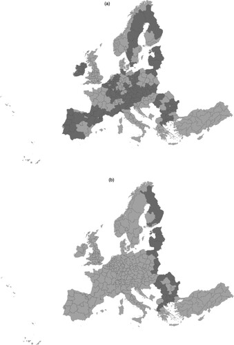
As additional variables in our model we consider dummy variables that indicate whether the region includes the national capital city, and if it is an internal or external border region. In our analysis, border regions are identified at the NUTS-2 level. Around the 48% of the regions under consideration are internal border areas (i.e., 117 regions), while around the 10% of these regions (i.e., 24 regions) are located on external borders. A map of border regions is presented in Figure 1. Dark grey indicates the border regions.

Figure 1. Internal border (a) and external border (b) European Union NUTS-2 regions.

Note: Dark grey indicates the border regions.

The variables under consideration are modelled through the SDM specification that is supported by the developed theoretical model. As a robustness check, this specification is compared with the spatial lag and the spatial error specifications. To this end, we use the Lagrange multiplier (LM) tests, in their classic and robust versions, which are based on the residuals of the ordinary least squares (OLS) model (Elhorst, 2010). According to the approach introduced by Elhorst (2010), when, based on the LM tests, the spatial lag, the spatial error model or both these specifications are preferable to the OLS model, the SDM specification should be estimated. Moreover, when these spatial models are estimated by maximum likelihood (ML), likelihood ratio (LR) tests can subsequently be used to verify two different hypotheses. The first hypothesis concerns whether the SDM can be simplified by a spatial lag model; the second hypothesis concerns whether the SDM could be simplified by a spatial error specification. The latter hypothesis corresponds to the common factor hypothesis. Results for LM and LR tests are reported in Table 2.

Table 2. Lagrange multiplier (LM) tests on spatial dependence and spatial error autocorrelation, likelihood ratio (LR) tests on parameter restrictions.

LMerror	72.9600***
LMlag	86.5100***
Robust LMerror	7.9290***
Robust LMlag	21.4700***
LRerr	20.4000***
LRlag	22.2100***

Note: Significance: ***1%, **5% and *10%.

Results for the classic LM tests indicate that the OLS model should be rejected in favour of both the spatial specifications, and, similarly, both the robust LM tests are highly significant. These results indicate that the SDM specification should be estimated. Results for the LR_err test show that the common factor hypothesis is rejected and, similarly, the LR_lag test is significant. These results confirm the appropriateness of the SDM specification.

The ML estimates for the SDM specification are reported in Table 3. The standard OLS estimates of the model are also presented, together with some diagnostics and performance measures. As shown, the coefficients associated with the initial level of GDP per worker, the capital city and the internal border dummy variables are significant in the non-spatial model. Furthermore, the signs of the coefficients are as expected for all explanatory variables, with the only exception of the working population growth rate. The coefficient associated with the capital city dummy variable expresses the differences in growth between the regions where the national capital cities are located and the other regions, given the other characteristics. The coefficient estimate is positive and statistically significant indicating the presence of a slight difference in the growth rate of GDP per worker between the regions where the capital cities are located and other regions, with the first ones overperforming with respect to the second ones. Similar considerations apply to the coefficient associated with the internal border dummy variable that indicates a growth rate of GDP per worker slightly higher in the internal border areas than in the other regional units. The coefficient associated with the external border dummy is negative, but it is not statistically significant. The goodness of fit of the model measured in term of $R^2$ is around 0.60, and the Moran’s $I$ test is highly significant, giving evidence of the presence of spatial dependence.

Table 3. Estimates for ordinary least squares (OLS) and the spatial Durbin model (SDM).

Variable	OLS	SDM
Constant	0.2750*** (0.0225)	0.1600*** (0.0329)
GDP per worker ($\mathrm{l}\mathrm{n}{y}_{i0}$)	−0.0236*** (0.0017)	−0.0130*** (0.0023)
Inequality ($\mathrm{l}\mathrm{n}Ine{q}_{i0}$)	0.0004 (0.0004)	0.0001 (0.0003)
Human capital $\left(\mathrm{l}\mathrm{n}{s}_i^H\right)$	0.0005 (0.0015)	0.0043** (0.0020)
$\mathrm{l}\mathrm{n}\left(n_i+0.05\right)$	0.0001 (0.0034)	−0.0156*** (0.0037)
$C{C}_i$	0.0134*** (0.0018)	0.0102*** (0.0016)
$I{B}_i$	0.0044*** (0.0010)	0.0020** (0.0009)
$E{B}_i$	−0.0013 (0.0021)	−0.0029* (0.0017)
lag GDP per worker		0.0002 (0.0033)
lag Inequality		0.0003 (0.0010)
lag Human capital		−0.0062** (0.0025)
$\mathrm{L}\mathrm{a}\mathrm{g}\mathrm{l}\mathrm{n}\left(n_i+0.05\right)$		0.0206*** (0.0053)
$\rho$		0.5635*** (0.0690)
$\lambda$ (convergence rate)	2.8648%	1.4349%
Moran’s I	0.2759***
Jarque–Bera test (normality)	69.9300***
Breusch–Pagan test (heterogeneity)	85.5900***
Studentized Breusch–Pagan test (heterogeneity)	41.1500***
Number of observations	245	245
R^2	0.6070
Akaike information criterion (AIC)	−1678.36	−1764.10

Notes: GDP, gross domestic product.

Standard errors are shown in parentheses. Significance: ***1%, **5% and *10%.

Moving to the SDM specification, all coefficients associated with the independent variables have the expected sign, with the only exception of the coefficient associated with the spatial lag of the inequality variable. The coefficient associated with this variable is not statistically significant as well as the coefficient associated with the inequality variable and the spatial lag of the initial level of GDP per worker. The coefficients associated with the dummy variables in the model are all significant. The positive sign of the coefficients associated with the capital city and the internal border dummy variables reveal that both these categories of regions overperform the other regions in the GDP per worker growth rate. The negative sign of the coefficient associated with the external border dummy variable shows that being located on the external border negatively impacts on the regional growth performances.

A lower value of the Akaike information criterion (AIC) indicates an improvement in the goodness of fit of the spatial specification with respect to the non-spatial one. Both the specifications indicate that a convergence process is taking place among the considered regions, but the inclusion of spatial effects tends to reduce the estimated speed of convergence.

As pointed out by LeSage and Pace (2009), in order to correctly interpret the SDM coefficients, the computation of direct, indirect and total impacts is needed. In fact, because of the spatial dependence effect that is incorporated in the model, a change in an explanatory variable for a single spatial unit has a direct impact on the dependent variable at the same location and could indirectly affect the dependent variable at different locations. The average direct impact provides a summary measure of the impact arising from changes in the $i$-th observation of a covariate on the dependent variable of the $i$-th region, and also includes feedback influences. The average indirect impact reflects spatial spillovers. The sum of the average direct and indirect impacts measures the average total impact. Table 4 reports the average direct, indirect, and total impacts that would arise from changing each explanatory variable in the SDM specification. A set of 2000 Monte Carlo (MC) draws is used to produce the impact estimates along with inferences regarding their statistical significance.

Table 4. Average impacts for the spatial Durbin model (SDM).

Variable	Average direct impact	Average indirect impact	Average total impact
GDP per worker ($\mathrm{l}\mathrm{n}{y}_{i0}$)	−0.0138***	−0.0155***	−0.0293***
Inequality ($\mathrm{l}\mathrm{n}Ine{q}_{i0}$)	0.0001	0.0008	0.0009
Human capital $\left(\mathrm{l}\mathrm{n}{s}_i^H\right)$	0.0039**	−0.0082**	−0.0043
$\mathrm{l}\mathrm{n}\left(n_i+0.05\right)$	−0.0144***	0.0259**	0.0115

Notes: GDP, gross domestic product.

Significance: ***1%, **5% and *10%.

A comparison between the average direct impacts in Table 4 and the parameter estimates in Table 3 reveals that these estimates have the same signs and are similar in magnitude. The slight differences between the two sets of estimates are due to feedback effects (Fischer, 2011).

The average indirect impact estimates for the human capital and the population growth rate are significant and have the expected signs. The average indirect impact associated with the initial level of GDP per worker is negative and significant, while the average indirect impact estimate for the inequality variable is positive but not significant. The average total impact estimates are significant only for the initial level of GDP per worker.

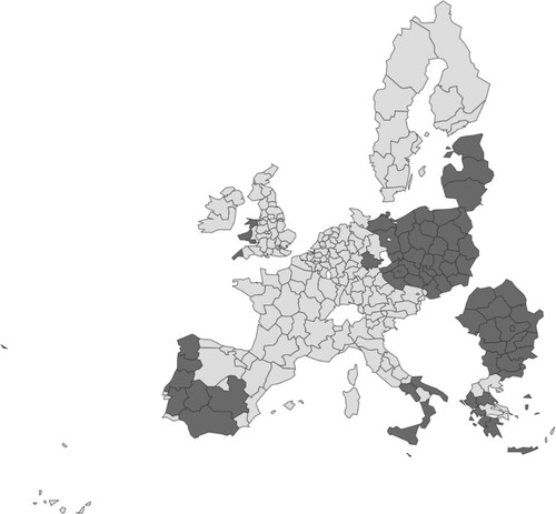
To account for spatial heterogeneity, we estimate the SDM model for two different clusters of regions corresponding to regions that are covered by the convergence objective and regions that are not covered by the convergence objective. A spatial map of these two clusters is shown in Figure 2. Dark grey indicates regions that are covered by the convergence objective. Light grey is used for non-convergence regions.

Figure 2. Convergence objective regions (dark grey) and non-convergence objective regions (light grey) identified according to the European Union's Cohesion Policy (2007–13).

Estimation results for the identified spatial clusters are reported in Table 5. As shown, some differences in the parameter estimates emerge between the two clusters of regions. The coefficient associated with the initial level of GDP per worker is negative and significant for both clusters, indicating that a convergence process is taking place in both these groups of regions. However, the speed of convergence for less developed regions is higher with respect to that reported for the more developed regions. This result indicates that economic growth proceeds faster in less developed regions than in other regions, and this circumstance could be partly attributed to the presence of EU funding in support of these regions. The coefficient associated with the inequality variable is positive and significant only for the cluster of less developed regions. This result indicates that, for this group of regions, inequality positively impacts on the process of economic growth. This result is consistent with the empirical findings in De Dominicis (2014). As a further result, we obtain that the human capital positively impacts on growth, but this effect is only significant for more developed regions. The coefficient associated with the population growth rate is negative and significant for both clusters of regions. The coefficients associated with the dummy variables reveal that the presence of the national capital city has a significant positive impact on regional growth for both more developed and less developed regions. Being located on the internal borders appears to influence regional growth positively, but this effect is significant only for more developed regions. Conversely, being located on the external border appears as detrimental for growth, but this negative impact is only significant for less developed regions. All coefficients associated with the spatially lagged explanatory variables have the expected sign in the cluster of regions not covered by the convergence objective. However, the coefficients associated with the spatial lag of the initial level of GDP per worker and with the spatial lag of the inequality variable are not significant. For less developed regions, the coefficient associated with the spatially lagged inequality variable is positive and statistically significant, revealing that the inequality observed in neighbour regions positively impact on growth in a particular region. As further results, we can note that the spatial autocorrelation parameter is positive and highly significant, and the AIC reveals that the goodness of fit of the model is improved in the heterogeneous model, with respect to the homogeneous one. These results point out the importance of accounting for both the heterogeneity and the spatial dependence of observations.

Table 5. Parameter estimates for spatial regimes, convergence objective versus non-convergence objective regions.

Variable	SDM: non-convergence objective	SDM: convergence objective
Constant	0.0753 (0.0499)	0.3625*** (0.0562)
GDP per worker ($\mathrm{l}\mathrm{n}{y}_{i0}$)	−0.0054* (0.0030)	−0.0246*** (0.0038)
Inequality ($\mathrm{l}\mathrm{n}Ine{q}_{i0}$)	−0.0003 (0.0003)	0.0017** (0.0007)
Human capital $\left(\mathrm{l}\mathrm{n}{s}_i^H\right)$	0.0077*** (0.0025)	0.0017 (0.0027)
$\mathrm{l}\mathrm{n}\left(n_i+0.05\right)$	−0.0193*** (0.0056)	−0.0145*** (0.0044)
$C{C}_i$	0.0058*** (0.0020)	0.0192*** (0.0025)
$I{B}_i$	0.0024** (0.0010)	0.0002 (0.0015)
$E{B}_i$	−0.0049 (0.0031)	−0.0049** (0.0021)
lag GDP per worker	0.0011 (0.0043)	−0.0052 (0.0049)
lag inequality	−0.0008 (0.0011)	0.0050** (0.0024)
lag human capital	−0.0075*** (0.0029)	−0.0098** (0.0046)
$\mathrm{L}\mathrm{a}\mathrm{g}\mathrm{l}\mathrm{n}\left(n_i+0.05\right)$	0.0299*** (0.0080)	0.0058 (0.0069)
Overall $\rho$	0.2977*** (0.0874)
$\lambda$ (convergence rate)	0.5615%	3.0157%
Number of observations	175	70
Akaike information criterion (AIC)	−1803.20
Chow test (overall stability)	4.5548***
Individual stability test for constant	12.1123**
Individual stability test GDP per worker	14.2903***
Individual stability test inequality	5.4865**
Individual stability test human capital	2.5201
Individual stability test $\mathrm{l}\mathrm{n}\left(n_i+0.05\right)$	0.5097
Individual stability test $C{C}_i$	17.6879***
Individual stability test $I{B}_i$	1.0215
Individual stability test $E{B}_i$	−0.0009

Notes: GDP, gross domestic product; SDM, spatial Durbin model.

Standard errors are shown in parentheses. Significance: ***1%, **5% and *10%.

In order to evaluate the significance of the identified spatial clusters, we can use the Chow test (Chow, 1960). The null hypothesis of the test is that the vector of parameters is constant. This test is implemented for all model parameters jointly (overall stability test) as well as for each parameter separately (individual stability test). Results for the overall stability test reveal that the spatial Chow test is highly significant, giving support to the idea of considering spatial regimes to control for spatial heterogeneity. Concerning the individual stability tests, we can observe that tests on the equality of the coefficients associated with the initial level of GDP per worker, with the inequality variable and with the capital city dummy variable are significant. This evidence shows that the spatial heterogeneity present in the considered regions is mainly due to the joint effect of these variables.

For the correct interpretation of the SDM coefficients we refer to direct, indirect and total impacts that, for both the identified spatial clusters, are reported in Table 6. For both groups of regions, the average direct impacts have the same sign as the parameter estimates (Table 5). The results reveal that the human capital is a growth promoting factor in more developed regions, while does not have a significant direct effect in less developed regions. Conversely, inequality positively impacts on growth in less developed regions, while does not have a significant direct effect on growth in more developed areas. For more developed regions, the average indirect effects reveal significant spatial spillovers for the human capital variable (positive indirect effect) and for the population growth rate (negative indirect effect). In regions covered by the convergence objective, significant spatial spillover effects are associated with the initial level of GDP per worker (negative indirect effect), the inequality variable (positive indirect effect), and the population growth rate (negative indirect effect).

Table 6. Average impacts for spatial regimes, convergence objective versus non-convergence objective regions.

Variable	SDM: non-convergence objective			SDM: convergence objective
	Average direct impact	Average indirect impact	Average total impact	Average direct impact	Average indirect impact	Average total impact
GDP per worker ($\mathrm{l}\mathrm{n}{y}_{i0}$)	−0.0055*	−0.0022	−0.0077*	−0.0249***	−0.0101**	−0.0350***
Inequality ($\mathrm{l}\mathrm{n}Ine{q}_{i0}$)	−0.0003	−0.0001	−0.0004	0.0017**	0.0007*	0.0024**
Human capital $\left(\mathrm{l}\mathrm{n}{s}_i^H\right)$	0.0078***	0.0032*	0.0110***	0.0017	0.0007	0.0024
$\mathrm{l}\mathrm{n}\left(n_i+0.05\right)$	−0.0195***	−0.0079*	−0.0274***	−0.0147***	−0.0060*	−0.0207***

Notes: GDP, gross domestic product; SDM, spatial Durbin model.

Significance: ***1%, **5% and *10%.

These empirical results suggest that that differences in the level of development of regions could determine differences in the factors driving regional growth. In fact, the positive impact of inequality on regional growth that is assumed in our theoretical model is only verified for less developed regions. Modelling spatial heterogeneity in the proposed model allows to appreciate the differences between the convergence-objective and the non-convergence objective regions, and to confirm the assumed relationship between inequality and regional growth relatively to the first group.

The positive relationship between inequality and growth is significant at the earlier stages of development because of the main role played by physical capital accumulation on regional growth (Galor & Moav, 2004). Hence, the mechanism according to higher inequality stimulates higher saving and physical capital accumulation, and thus growth, is verified for less developed regions. Conversely, in more developed economies, the human capital accumulation appears to replace physical capital accumulation as a growth promoting factor (Galor & Moav, 2004). Our empirical results support this evidence, revealing a significant and positive effect of human capital on growth only for transition and more developed regions.

Our empirical results partly confirm empirical findings in the previous literature. Like in De Dominicis (2014) our empirical evidence shows the growth promoting effect of a relatively concentrated distribution of GDP at lower level of development. Unlike De Dominicis (2014), we found a positive and significant spillover effect associated with the inequality variable for less developed regions. This implies that, at lower levels of development, the initial internal disparities in neighbour regions have a positive impact on economic growth in a particular region. Our results confirm the empirical evidence in De Dominicis (2014) about the role of inequality in more developed regions. In fact, like in the De Dominicis (2014), our empirical results indicate, for this group of regions, not significant impacts of inequality on regional growth. This suggests that initial regional disparities in more advanced regional economies do not exert a role in enhancing regional growth. However, our analysis provides new evidence for less developed regions, by isolating the actual inequality (i.e., the component of inequality that is not influenced by spatial dependence) from the component of inequality that is influenced by regional interdependencies driven by geographical proximity.

The different impacts of inequality on growth for different groups of regions suggest the existence of several factors underlying the distinctive growth experiences. In fact, the differences in the economic convergence process experienced by regions result from their different levels of development and from the interactions among policy and institutional aspects, as well as among historical and geographical factors characterizing the regional units. Raising the awareness about these differences among regions could be useful in promoting place-based policies, which focus on the peculiarities and the specific needs of territories.

CONCLUSIONS

In this paper we developed a theoretical model that relates inequality and regional growth, explicitly taking into account the spatial interactions among regions. The proposed model extends the spatial MRW model developed by Fischer (2011), introducing inequality among the explanatory variables. The physical capital investment rate is expressed as a function of inequality, based on the assumption that higher inequality enhances investments from richer regions, while the redistribution of resources from rich to poor regions, determines a decreasing of savings and investments (De Dominicis, 2014).

The proposed specification includes the spatial lag of the exogenous variables as well as the spatial lag of the endogenous variable and is referred to as the spatial Durbin model (LeSage & Pace, 2009). The inequality variable included in the model specification is derived by the spatial decomposition of the Gini index proposed by Rey and Smith (2013).

Our theoretical model states that the growth rate of output in a regional economy depends positively on inequality in the region and negatively on inequality in neighbouring regions. By taking into account the spatial interactions among regions, the predictions of our model allow a better understanding of the role played by geographical location and spatial externalities in regional growth and in its link with income inequality.

The proposed model is tested focusing on 245 NUTS-2 regions across 22 European countries, over the period 2003–16. Results from test on parameter restrictions confirm the appropriateness of the proposed specification, and the empirical estimates mainly support the theoretical model. The coefficient associated with the inequality variable is not significant when considering the homogeneous model. Assuming two different spatial regimes, identified according to the eligibility of regions for EU funds under the convergence objective, reveals differences in the growth process as well as in the growth promoting factors. Specifically, we found that in less developed regions the converge process is taking place at a faster rate than that obtained for the more developed regions. This result could be explained by the EU policy that support convergence in poorer areas, but also by the combination of different factors that exert a growth promoting effect. Specifically, the initial internal disparities appear to enhance growth in less developed regions, while do not play a significant role in wealthy regional economies. In this latter group of regions, the investment in human capital has a positive impact on growth, while it does not have a significant effect on growth at lower level of development. These differences emerge only when spatial similarity is considered jointly with regional peculiarities, and confirm the relevance of place-based policies, differentiated according to the specific needs of regional economies. The identification of two separate clusters, corresponding to different levels of regional development, facilitate a deeper understanding of the impact of inequality on growth in different regional economies. A further step, in the future research, might consist in introducing these differences in the definition of the proximity relationships. This would imply assigning different spatial weights to neighbour regions according to their level of development.

To proper extract the influence of neighbour regions, such proximity matrices could be also defined differentiating among the neighbour units that belong to the same or a different country with respect to the region under consideration. Defining proximity structures based on these criteria would allow to summarize in a single matrix specific effects that in our model are introduced by using dummy variables and spatial clustering.

DISCLOSURE STATEMENT

No potential conflict of interest was reported by the author(s).

Additional information

Funding

This study was financed by the project H2020 IMAJINE, which received funding from the European Union's Horizon 2020 Research and Innovation Programme [grant agreement number 726950]. This paper reflects only the authors' view. The European Commission is not responsible for any use that may be made of the information the paper contains.

Notes

1. Given the SDM specification $Y=\rho WY+X\text{β}+WX\theta +ϵ$, with $\rho$, $\text{β}$ and $\theta$ denoting the parameters associated with the spatially lagged endogenous explanatory variable, with the exogenous explanatory variable and with the spatially lagged exogenous explanatory variables, respectively, the spatial error specification is derived by imposing the following parameter restriction: $\theta =-\rho \text{β}$.

2. The NUTS-2 regions that, because of missing data, are excluded by the analysis are the five regions belonging to Denmark, two regions of Germany: Chemnitz and Leipzig; two regions of Spain: Ciudad Autonoma de Ceuta and Ciudad Autonoma de Melilla; the five overseas Departments in France; Cyprus; the two regions of Slovenia; the two regions of Croatia; the seven regions of Hungary; and the one region of the UK: Highlands and Islands. The region of London is partitioned into Inner London and Outer London, according to the 2010 NUTS classification. For the identification of all other NUTS-2 regions, we refer to the 2013 NUTS classification. Luxembourg is excluded from the analysis because of the coincidence between the NUTS-2 and NUTS-3 levels of classification, which does not allow the calculation of the within-component of inequality.

3. Among the EU NUTS-2 regions there are some regions composed by a relatively large number of NUTS-3 regions, and other regions composed by only one NUTS-3 region. For the latter regions, the Gini index assumes a value of 0. In order to include also these regions in our analysis, we follow the same approach proposed by De Dominicis (2014), and when a NUTS-2 region is composed by only one NUTS-3 region, we assign to the region a value of the Gini index equal to the average of the Gini index computed for the NUTS-2 regions in the same country.

4. Estimation results obtained for these different specifications of the proximity matrix are available from the authors upon request.

REFERENCES

- Alesina, A., & Rodrik, D. (1994). Distributive politics and economic growth. The Quarterly Journal of Economics, 109(2), 465–490. https://doi.org/https://doi.org/10.2307/2118470
- Anderson, J., & van Wincoop, E. (2003). Gravity with gravitas: A solution to the border puzzle. American Economic Review, 93(1), 170–192. https://doi.org/https://doi.org/10.1257/000282803321455214
- Anselin, L. (1988). Spatial econometrics: Methods and models. Kluwer.
- Anselin, L., & Rey, S. J. (1991). Properties of tests for spatial dependence in linear regression models. Geographical Analysis, 23(2), 112–131. https://doi.org/https://doi.org/10.1111/j.1538-4632.1991.tb00228.x
- Arbia, G. (2001). The role of spatial effects in the empirical analysis of regional concentration. Journal of Geographical Systems, 3(3), 271–281. https://doi.org/https://doi.org/10.1007/PL00011480
- Artelaris, P., & Petrakos, G. (2016). Intraregional spatial inequalities and regional income level in the European Union: Beyond the inverted-U hypothesis. International Regional Science Review, 39(3), 291–317. https://doi.org/https://doi.org/10.1177/0160017614532652
- Bailey, N., Holly, S., & Pesaran, M. H. (2016). A two-stage approach to spatio-temporal analysis with strong and weak cross-sectional dependence. Journal of Applied Econometrics, 31(1), 249–280. https://doi.org/https://doi.org/10.1002/jae.2468
- Basile, R., Durbán, M., Mínguez, R., Montero, J. M., & Mur, J. (2014). Modeling regional economic dynamics: Spatial dependence, spatial heterogeneity and nonlinearities. Journal of Economic Dynamics and Control, 48, 229–245. https://doi.org/https://doi.org/10.1016/j.jedc.2014.06.011
- Basile, R., & Gress, B. (2005). Semi-parametric spatial auto-covariance models of regional growth behaviour in Europe. Région et Développement, 21, 93–118.
- Butkus, M., Cibulskiene, D., Maciulyte-Sniukiene, A., & Matuzeviciute, K. (2018). What is the evolution of convergence in the EU? Decomposing EU disparities up to the NUTS 3 level. Sustainability, 10(5), 1–37. https://doi.org/https://doi.org/10.3390/su10051552
- Capello, R., Caragliu, A., & Fratesi, U. (2018). Measuring border effects in European cross-border regions. Regional Studies, 52(7), 986–996. https://doi.org/https://doi.org/10.1080/00343404.2017.1364843
- Chen, B. (2003). An inverted-U relationship between inequality and long-run growth. Economics Letters, 78(2), 205–212. https://doi.org/https://doi.org/10.1016/S0165-1765(02)00221-5
- Chow, G. C. (1960). Tests of equality between sets of coefficients in two linear regressions. Econometrica, 28(3), 591–605. https://doi.org/https://doi.org/10.2307/1910133
- Crespo Cuaresma, J., Doppelhofer, G., & Feldkircher, M. (2014). The determinants of economic growth in European regions. Regional Studies, 48(1), 44–67. https://doi.org/https://doi.org/10.1080/00343404.2012.678824
- De Dominicis, L. (2014). Inequality and growth in European regions: Toward a place-based approach. Spatial Economic Analysis, 9(2), 120–141. https://doi.org/https://doi.org/10.1080/17421772.2014.891157
- Durlauf, S. N., & Johnson, P. A. (1995). Multiple regimes and cross-country growth behaviour. Journal of Applied Econometrics, 10(4), 365–384. https://doi.org/https://doi.org/10.1002/jae.3950100404
- Elhorst, J. P. (2010). Applied spatial econometrics: Raising the bar. Spatial Economic Analysis, 5(1), 9–28. https://doi.org/https://doi.org/10.1080/17421770903541772
- Ertur, C., & Koch, W. (2007). Growth, technological interdependence and spatial externalities: Theory and evidence. Journal of Applied Econometrics, 22(6), 1033–1062. https://doi.org/https://doi.org/10.1002/jae.963
- Ertur, C., Le Gallo, J., & Baumont, C. (2006). The European regional convergence process, 1980–1995: Do spatial regimes and spatial dependence matter? International Regional Science Review, 29(1), 3–34. https://doi.org/https://doi.org/10.1177/0160017605279453
- Eurostat. (2019). Methodological manual on territorial typologies (2018 ed.). Publication Office of the European Union.
- Ezcurra, R., & Rodríguez-Pose, A. (2013). Does economic globalization affect regional inequality? A cross-country analysis. World Development, 52(1), 92–103. https://doi.org/https://doi.org/10.1016/j.worlddev.2013.07.002
- Ezcurra, R., & Rodríguez-Pose, A. (2014). Trade openness and spatial inequality in emerging countries. Spatial Economic Analysis, 9(2), 162–182. https://doi.org/https://doi.org/10.1080/17421772.2014.891155
- Fischer, M. M. (2011). A spatial Mankiw–Romer–Weil model: Theory and evidence. The Annals of Regional Science, 47(2), 419–436. https://doi.org/https://doi.org/10.1007/s00168-010-0384-6
- Forbes, K. J. (2000). A reassessment of the relationship between inequality and growth. American Economic Review, 90(4), 869–887. https://doi.org/https://doi.org/10.1257/aer.90.4.869
- Galor, O. (2000). Income distribution and the process of development. European Economic Review, 44(4–6), 706–712. https://doi.org/https://doi.org/10.1016/S0014-2921(99)00039-2
- Galor, O., & Moav, O. (2004). From physical to human capital accumulation: Inequality and the process of development. Review of Economic Studies, 71(4), 1001–1026. https://doi.org/https://doi.org/10.1111/0034-6527.00312
- Henderson, J. V., Squires, T. L., Storeygard, A., & Weil, D. N. (2018). The global spatial distribution of economic activity: Nature, history and the role of trade. The Quarterly Journal of Economics, 133(1), 357–406. https://doi.org/https://doi.org/10.1093/qje/qjx030
- Iammarino, S., Rodríguez-Pose, A., & Storper, M. (2019). Regional inequality in Europe: Evidence, theory and policy implications. Journal of Economic Geography, 19(2), 273–298. https://doi.org/https://doi.org/10.1093/jeg/lby021
- Janikas, M. V., & Rey, S. J. (2008). On the relationships between spatial clustering, inequality, and economic growth in the United States: 1969–2000. Region et Développement, 27, 13–34.
- Kaldor, N. (1956). Alternative theories of distribution. The Review of Economic Studies, 23(2), 83–100. https://doi.org/https://doi.org/10.2307/2296292
- Kashiha, M., Depken, C., & Thill, J.-C. (2016). Border effects in a free-trade zone: Evidence from European wine shipments. Journal of Economic Geography, 17, 411–433. https://doi.org/https://doi.org/10.1093/jeg/lbw017
- Koo, J., & Song, Y. (2016). The relationship between income inequality and aggregate saving: An empirical analysis using cross-country panel data. Applied Economics, 48(10), 892–901. https://doi.org/https://doi.org/10.1080/00036846.2015.1090548
- Le Gallo, J., & Ertur, C. (2003). Exploratory spatial data analysis of the distribution of regional per capita GDP in Europe, 1980–1995. Papers in Regional Science, 82(2), 175–201. https://doi.org/https://doi.org/10.1007/s101100300145
- LeSage, J., & Pace, K. (2009). Introduction to spatial econometrics. CRC Press.
- Lessmann, C. (2014). Spatial inequality and development. Is there an inverted-U relationship? Journal of Development Economics, 106(C), 35–51. https://doi.org/https://doi.org/10.1016/j.jdeveco.2013.08.011
- Lessmann, C., & Seidel, A. (2017). Reginal inequality, convergence, and its determinants. A view from outer space. European Economic Review, 92(1), 110–132. https://doi.org/https://doi.org/10.1016/j.euroecorev.2016.11.009
- Li, H., & Zou, H. (1998). Income inequality is not harmful for growth: Theory and evidence. Review of Development Economics, 2(3), 318–334. https://doi.org/https://doi.org/10.1111/1467-9361.00045
- Mankiw, N. G., Romer, D., & Weil, D. N. (1992). A contribution to the empirics of economic growth. The Quarterly Journal of Economics, 107, 407–437. https://doi.org/https://doi.org/10.2307/2118477
- Márquez, M. A., Lasarte-Navamuel, E., & Lufin, M. (2019). The role of neighborhood in the analysis of spatial economic inequality. Social Indicators Research, 141(1), 245–273. https://doi.org/https://doi.org/10.1007/s11205-017-1814-y
- Martino, C., & Perugini, G. (2008). Income inequality within European regions: Determinants and effects on growth. Review of Income and Wealth, 3, 373–406. https://doi.org/https://doi.org/10.1111/j.1475-4991.2008.00280.x
- McCallum, J. (1995). National borders matter: Canada–U.S. regional trade patterns. American Economic Review, 85(3), 615–623.
- McMillen, D. P. (2012). Perspectives on spatial econometrics: Linear smoothing with structured models. Journal of Regional Science, 52(2), 192–209. https://doi.org/https://doi.org/10.1111/j.1467-9787.2011.00746.x
- Mookherjee, D., & Shorrocks, A. (1982). A decomposition analysis of the trend in UK income inequality. The Economic Journal, 92(368), 886–902. https://doi.org/https://doi.org/10.2307/2232673
- Panizza, U. (2002). Income inequality and economic growth: Evidence from American data. Journal of Economic Growth, 7(1), 25–41. https://doi.org/https://doi.org/10.1023/A:1013414509803
- Panzera, D., & Postiglione, P. (2020). Measuring the spatial dimension of regional inequality: An approach based on the Gini correlation measure. Social Indicators Research, 148(2), 379–394. https://doi.org/https://doi.org/10.1007/s11205-019-02208-7
- Partridge, M. D. (2005). Does income distribution affect U.S. state economic growth? Journal of Regional Science, 45(2), 363–394. https://doi.org/https://doi.org/10.1111/j.0022-4146.2005.00375.x
- Persson, T., & Tabellini, G. (1994). Is inequality harmful for growth? American Economic Review, 84, 600–621. https://doi.org/https://doi.org/10.3386/w3599
- Pesaran, M. H. (2015). Testing weak cross-section dependence in large panels. Econometric Reviews, 34(6–10), 1089–1117. https://doi.org/https://doi.org/10.1080/07474938.2014.956623
- Petrakos, G., Rodríguez-Pose, A., & Rovolis, A. (2005). Growth, integration, and regional disparities in the European Union. Environment and Planning A: Economy and Space, 37(10), 1837–1855. https://doi.org/https://doi.org/10.1068/a37348
- Portnov, B. A., & Felsenstein, D. (2010). On the suitability of income inequality measures for regional analysis: Some evidence from simulation analysis and bootstrapping tests. Socio-Economic Planning Sciences, 44(4), 212–219. https://doi.org/https://doi.org/10.1016/j.seps.2010.04.002
- Postiglione, P., Andreano, M. S., & Benedetti, R. (2013). Using constrained optimization for the identification of convergence clubs. Computational Economics, 42(2), 151–174. https://doi.org/https://doi.org/10.1007/s10614-012-9325-z
- Postiglione, P., Benedetti, R., & Lafratta, G. (2010). A regression tree algorithm for the identification of convergence clubs. Computational Statistics & Data Analysis, 54(11), 2776–2785. https://doi.org/https://doi.org/10.1016/j.csda.2009.04.006
- Quah, D. (1997). Empirics for growth and distribution: Stratification, polarization and convergence clubs. Journal of Economic Growth, 2(1), 27–59. https://doi.org/https://doi.org/10.1023/A:1009781613339
- Rey, S. J., & Janikas, M. V. (2005). Regional convergence, inequality, and space. Journal of Economic Geography, 5(2), 155–176. https://doi.org/https://doi.org/10.1093/jnlecg/lbh044
- Rey, S. J., & Smith, R. J. (2013). A spatial decomposition of the Gini coefficient. Letters in Spatial and Resource Sciences, 6(2), 55–70. https://doi.org/https://doi.org/10.1007/s12076-012-0086-z
- Rodríguez-Pose, A. (2012). Trade and regional inequality. Economic Geography, 88(2), 109–136. https://doi.org/https://doi.org/10.1111/j.1944-8287.2012.01147.x
- Shorrocks, A., & Wan, G. (2005). Spatial decomposition of inequality. Journal of Economic Geography, 5(1), 59–81. https://doi.org/https://doi.org/10.1093/jnlecg/lbh054
- Theil, H. (1967). Economics and information theory. North Holland.
- Thorbecke, E., & Charumilind, C. (2002). Economic inequality and its socioeconomic impact. World Development, 30(9), 1477–1495. https://doi.org/https://doi.org/10.1016/S0305-750X(02)00052-9