A trade hierarchy of cities based on transport cost thresholds

ABSTRACT

Empirical evidence has been lacking to explain trade agglomerations within countries. Starting with a novel micro-database of road freight shipments between Spanish municipalities for the period 2003–07, we break down city (municipal) trade flows into the extensive and intensive margins and assess trade frictions and trade concentration relying on a unique generalized transport cost measure and three internal borders: NUTS-5 (municipal), NUTS-3 (provincial) and NUTS-2 (regional). We find a stark accumulation of trade flows up to a transport cost value of €189 (approximately 170 km) and conclude that this high density is not due to administrative borders effects but to significant changes in the trade-to-transport costs relationship. To support this hypothesis, we propose and conduct an endogenous Chow test to identify significant thresholds at which trade flows change structurally with transport costs. These breakpoints allow us to split the sample when controlling for internal borders, and to define trade market areas corresponding to specific transport costs that consistently reveal an urban hierarchy of cities. The results provide clear evidence with which to corroborate the predictions of Central Place Theory.

KEYWORD:

• Municipal freight flows
• generalized transport costs
• breakpoints
• market areas
• urban hierarchy
• Central Place Theory

JEL:

• F14
• F15
• O18
• O20

INTRODUCTION

In the absence of reliable data, intra-national trade patterns are in general neither well understood nor well characterized. The lack of highly granular micro-data on inter-regional trade flows deters empirical analyses on why trade agglomerations occur in some places and not in others within a country.¹ Since the first empirical and seminal studies (Hillberry & Hummels, 2003; Wolf, 1997, 2000) up to more recent works (Andresen, 2010; Capello et al., 2018b; Martínez-San Román et al., 2017), there is a growing literature pointing out an internal home-bias effect as, inter alia, one of the key determinants of the location of economic activity within countries and intra-national trade agglomerations.

The causes and explanations for this intra-country effect are multiple. Whereas some studies focus on historical and cultural barriers to trade (Capello et al., 2018a; Nitsch & Wolf, 2013; Tubadji & Nijkamp, 2015; Wrona, 2018), hub-and-spoke structures (Gallego et al., 2015), transport-mode competitions within a country (Llano et al., 2017), or even the impediments raised by business networks (Garmendia et al., 2012), others emphasize unexpected increases in the internal border effect over the last decades (Crafts & Klein, 2014; Martínez-San Román et al., 2017). Not only these empirical factors but also prominent theoretical set-ups have been cited to ascribe the internal home-bias effect either to the fragmentation of global production chains in areas near international borders (Yi, 2010) or to spatial frictions between cities (Behrens et al., 2017).

Within this framework, the study by Hillberry and Hummels (2008) sheds light on the appearance of an internal home bias at the municipal level once accurate inter-regional trade flows and very precise measures of internal distance are used. Even if this trade concentration holds over short distances in their study, the authors conclude that the internal home bias is a reductio ad absurdum of the one observed at the international level. Departing from this finding, we argue that the internal home-bias effect not only is real but also results from breakpoint changes in the trade-to-transport costs relationship that shapes a series of trade market areas around a country’s largest trading cities.

More specifically, we find discontinuous changes between trade and transport costs that map successive and distance-increasing market areas which, as a result, give rise to a hierarchy of cities as predicted by Central Place Theory (CPT) (Hsu, 2012; Hsu et al., 2014; Mulligan et al., 2012; Parr, 2002; Tabuchi & Thisse, 2011; Taylor & Hoyler, 2021; Zhu et al., 2021).

To arrive at these conclusions, we have relied on two unique and very detailed databases: (1) a panel database (2003–07) on individual trade flows for Spanish municipalities; and (2) an additional bilateral panel database with the precise and realistic transport costs associated with these trade flows. With these databases we propose and adopt a new methodological approach within the trade literature to determine spatial breakpoints in trade flows caused by the changing nature of transport costs. The new method resorts to a stability econometric (Chow) test for structural changes, first introduced by Berthelemy and Varoudakis (1996). We apply this test to assess whether trade flows (structurally) change beyond a certain transport cost breakpoint. This information allows us to split internal distances by thresholds and introduce them into a standard gravity set-up. This new definition of internal distances is the basis, on one hand, to define cities’ market areas and, on the other, to accurately measure the internal home bias at different spatial levels for either the overall value of trade or its margins. Whereas we interpret the former under the insights of CPT and the consequent hierarchy of cities, we show that the latter leads to an overestimation of the (‘illusory’) internal border effect when transport costs are not correctly controlled for. Indeed, we argue that the arbitrary use of administrative boundaries as a spatial limitation to collect data and account for border effects becomes an aggregation artefact (Hillberry, 2002a; Llano-Verduras et al., 2011) that leads to misleading conclusions about the impediments to intra-national trade flows.

This paper contributes to and links with the literatures on intra-national trade flows and their associated system of city mapping. We show that it is not internal administrative borders that effectively hamper trade, but the change in the relationship between the trade flows and transport costs that generates the border effects achieved within a country. This is consistent with the removal of intra-national administrative impediments to trade through single-market agreements. We also contribute to the empirical study of trade-market areas, as intra-national economic boundaries depending on either their geographical reach (Löffler, 1998; Sohn & Licheron, 2018) or their shape throughout a hierarchy of cities (Hsu, 2012; Hsu et al., 2014; Taylor & Hoyler, 2021), and provide empirical evidence for the prominent and theoretical literature on trading cities (Anas & Xiong, 2003; Behrens et al., 2017; Cavailhes et al., 2007; Mori & Wrona, 2018). Finally, we develop further methodological approaches for highly granular gravity-trade models (Head & Mayer, 2014) and their crucial debate on the treatment of non-linear transport costs (Abbate et al., 2012; Gallego & Llano, 2014).

After reviewing the contributions of the study, we now outline our sequential research strategy. The first step compiles a novel database of road freight shipments consisting of micro-data for individual shipments between Spanish municipalities. This statistical information, drawn from the Spanish Road Freight Transportation Survey (RFTS), allows us to calculate the bilateral value of trade and decompose it into the extensive and intensive margins. Next, for each bilateral flow we compute the actual monetary transport cost, or generalized transport cost (GTC), which corresponds to the minimum economic cost between any origin and destination. This is the sum of distance-related costs (e.g., fuel, toll, tires) and time-related costs (e.g., salaries, insurance, taxes) for each route between any pair of Spanish municipalities. To calculate these GTC, we use the programming techniques available in Geographic Information Systems (Arc/GIS) which optimize for the lowest cost routes using the existing and digitized road networks for the period 2003–07. In contrast to all previous studies, which use the standard and non-monetary transport cost proxies of distance or travel time, we introduce a real euro and time-varying measure of the spatial frictions affecting trade.

Subsequently, we analyse transport costs and border impediments for the three intra-national administrative borders in Spain, that is, NUTS-5 (municipal), NUTS-3 (provincial) and NUTS-2 (regional), using the Poisson pseudo-maximum likelihood (PPML) estimator to control for pervasive zero-valued trade flows within the gravity model (Santos Silva & Tenreyro, 2006, 2010, 2011). The results show that municipal borders have a stronger impact on trade flows and extensive and intensive trade margins than the results reported by, among others, Hillberry and Hummels (2008). Provinces and regions, meanwhile, have a much weaker impact than the literature suggests (Requena & Llano, 2010). Thanks to the PPML estimator, we show that this spatial trade pattern is explained by the over-concentration of trade flows over short distances; therefore, the internal effect of administrative borders tends to be underestimated for short distances and overstressed for long ones.

To explain these results further, we introduce to the trade literature the method developed by Berthelemy and Varoudakis (1996) for endogenous economic growth models. They propose a stability Chow test to detect specific breakpoints shaping different structural models in their data. We adopt this test to detect differences in the trade-to-transport costs relationship and find that only breakpoints arise in the total value of trade and its extensive margin, not the intensive one, pointing out that the spatial concentration of trade flows is mainly driven by the extensive margin. Once we divide our transport costs measure into subsamples (distance intervals) and determine the existence of a series of statistically significant breakpoints, we split our PPML regressions by these new transport cost thresholds. This stands in contrast with, for example, Eaton and Kortum (2002) and Anderson and Yotov (2012), who segment trade flows by arbitrary distances. Thanks to these statistically defined transport-cost thresholds, we conclude both that the internal border effect is neither unique nor has a single non-linear quadratic impact on trade, as the literature emphasizes. Indeed, we argue that it is precisely the existence of such thresholds that truly raise internal impediments to trade, which eventually spill over several and consecutive administrative boundaries. To the best of our knowledge, this is the first analysis using a structural-break methodology for the trade-to-transport cost relationship in the trade literature.

Lastly, since the density of trade flows is geographically localized in short-distance thresholds and mainly driven by the extensive margin, we show that the resulting agglomeration economies shape a series of nested trade-market areas around increasingly large cities, giving rise to an urban hierarchy whose mapping coincides with the postulates of the CPT. Thus, we highlight that the so-called internal border effect is the consequence of higher order cities that act as supply centres for either their metropolitan areas or surrounding cities of lower rank, a relatively unexplored relationship in the empirical literature on urban areas. These empirical regularities are promising for future research linking trade and CPT.

The remainder of the paper is structured as follows. The next section explains the databases and the decomposition of trade flows. The third section presents the econometric analysis. The fourth section discusses the structural breakpoint methodology and its application to the gravity model of trade. The interpretation of our results in light of CPT and its associated hierarchy of cities is performed in the fifth section. The last section draws the main conclusions.

TRADE FLOWS, EXTENSIVE AND INTENSIVE MARGINS, AND TRANSPORT COSTS

Trade value data and the extensive and intensive margins

To build our value trade data we rely on a micro-database on freight flows by road: the Road Freight Transportation Survey (RFTS), compiled by the transport division of the Spanish Ministry of Transport, Mobility and Urban Agenda for the period 2003–07. This database is based on a randomly surveyed sample of freight companies and independent truckers with vehicles weighing more than 3.5 tons, which together account for almost 85% of all internal freight flows. It includes vehicle and shipment characteristics such as the type of commodity shipped, the number of tons carried by the truck, the number of shipments, and the distance travelled between any origin i and destination j, registered at the NUTS-5 municipal level.² For the 2003–07 period, the database contains more than 1,890,000 records (empty shipments included) which, on average, involve 7178 municipalities as origins and 7913 municipalities as destinations. However, most of them are municipalities with little relevance in terms of population and trade volumes. Therefore, we consider municipalities with more than 10,000 inhabitants in the period 2003–07. The final database consists of 633 municipalities whose freight trade volume by road represents 75.5% of the total freight flows.

Thanks to the RFTS micro-database we calculate the total value of trade and subsequently break it down into the extensive and the intensive margins. Adopting Hillberry and Hummels’ (2008) proposal, the total value of trade between each origin–destination ($T_{ijt}$) at time t can be decomposed as follows (dropping subscript t to avoid notational clutter): (1) $T_{ij}=N_{ij}{\overline{PQ}}_{ij}$(1) where $N_{ij}$ represents the total number of shipments (i.e., the extensive margin); and ${\overline{PQ}}_{ij}$ is the average value per shipment (i.e., intensive margin) composed of the mean of values of prices (${\overline{P}}_{ij}$) and tons (${\overline{Q}}_{ij}$).³

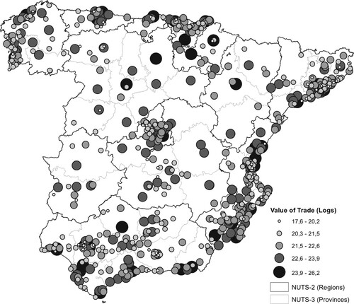
Figure 1 maps the total value of trade (in logarithms) for the 633 municipalities. The largest trade flows occur in areas with the highest levels of economic activity (Madrid, the Mediterranean coast and the Basque Country), whereas less populated areas (south-west and north-west) register trade only around largest cities. This spatial pattern is consistent with previous evidence on the concentration of Spanish international exporters (Ramos & Moral-Benito, 2017).

Figure 1. Logarithm of total value of trade for the 633 municipalities.

Note: Graduated map with averages for the period 2003–07.

Source: Authors’ own elaboration from the Spanish Road Freight Transportation Survey (RFTS) data.

Generalized transport cost (GTC): advantages over distance and time proxies

Another novel aspect of this study is the use of a monetary measure of transport cost that improves the proxies normally used in the literature, mainly geographical distance and travel time. This variable stands for a GTC definition corresponding to the least-cost itinerary between an origin and a destination, as discussed by Combes and Lafourcade (2005), Zofío et al. (2014) and Persyn et al. (2020).

In particular, we have calculated the specific GTCs that match the inter- and intra-municipal trade flows represented by door-to-door shipments. Unlike distance and travel time, the GTC differentiates economic costs related to both distance and time cost, and accounts for changes in transport operating costs, particularly those related to the transport service market (e.g., fuel prices) and regulatory and institutional conditions (e.g., mostly related to wages in the labour market).

In the GTCs methodology, it is assumed that the road freight firms providing the transportation service between any two locations minimize the economic costs. For a given origin $i$ and destination $j$ in year $t$, a least cost algorithm is implemented using the Arc/GIS Network Toolbox. The solution yields the optimal itinerary between them accounting for both physical and economic attributes.

We make use of a set of digitized road networks for 2003–07 containing information about these attributes for every road arc, $a$ (or segment) in a given year, $t$. As for the physical attributes, the main characteristics are capacity, gradient and congestion (upon which the arc speed depends). Regarding economic costs, these are related to the arc distance and travel time: $d_a^t$ and $t_a^t$ = $d_a^t$/$s_a^t$, where $s_a^t$ is the maximum speed in the arc, bounded by the legal limit. All economic costs are referred to the most representative vehicle (e.g., 80% of all transport services are performed with a 40 ton articulated truck), and vary by location $l$ and time period $t$, depending on where the arcs are located (e.g., rates for every tolled road are included, and yearly updated). The economic distance unit costs in time $t$, denoted by $e_k^t$, that is, euros/km, include the following variables: (1) fuel costs, denoted by $fue{l}_i^t$ (i.e., it is assumed that the tank is refilled in origin $i$ where the transport firm is located) – for long trips the average fuel price at origin and destination is used; (2) toll costs, $tol{l}_l^t$; (3) accommodation and allowance costs, $accomallo{w}_l^t$; (4) tire costs, $tir{e}_i^t$; and (5) vehicle maintenance and repairing operating costs, $repman{t}_i^t$. Taking into account these operating costs, the total distance cost corresponding to an itinerary $I_{ij}^t$ is: $\begin{array}{rl}Dist{C}_{ij}^t& =\sum _{a\in I_{ij}^t}\left(\sum _k{e}_k^t\right)d_a^t=\sum _{a\in I_{ij}^t}(fue{l}_i^t+tol{l}_l^t\\ & +accomallo{w}_l^t+tir{e}_i^t+repman{t}_l^t)d_a^t.\end{array}$Likewise, the economic unit costs associated with time, denoted by $e_h^t$, that is, euros/h, include the following variables (when the location subscript is omitted, it indicates that these are nationwide prices): (1) labour costs; $la{b}_i^t$; (2) financial costs associated with amortization, $amor{t}^t$; (3) financing, $fi{n}^t$; (4) insurance costs, $in{s}^t$; (5) taxes, $ta{x}_i^t$; and (6) indirect costs, $in{d}_i^t$, associated with other administration overhead, operating expenses and commercial costs. Given the driving time for an arc: $t_a^t$, the overall cost associated with travel the whole length of an itinerary is: $\begin{array}{rl}& Time{C}_{ij}^t=\left(\sum _l{e}_h^t\right)\left(\sum _{a\in {\mathrm{I}}_{ij}^t}{t}_a^t\right)=\left(\sum _l{e}_h^t\right)\left(\sum _{a\in I_{ij}^t}{\displaystyle \frac{d_a^t}{s_a^t}}\right)=\\ & =\left(la{b}_i^t+amor{t}^t+fi{n}^t+in{s}_{}^t+ta{x}_i^t+in{d}_i^t\right)\left(\sum _{a\in {\mathrm{I}}_{ij}^t}{\displaystyle \frac{d_a^t}{s_a^t}}\right).\end{array}$With this information we solve for the GTC, which is the solution to the following minimization problem that identifies the least cost route $I_{ij}^{t\ast }$ in period $t$, among the set of itineraries $I_{ij}^t$: $\begin{array}{rl}& GT{C}_{ij}^t=\underset{I_{ij}^t\in I_{ij}^t}{min}\left(Dist{C}_{ij}^t+Time{C}_{ij}^t\right)=\\ & =\sum _{a\in I_{ij}^t}\left(\sum _k{e}_k^t\right)d_a^t+\left(\sum _l{e}_h^t\right)\left(\sum _{a\in {\mathrm{I}}_{ij}^t}{t}_a^t\right)\\ & =\left(\sum _l{e}_h^t\right)\left(\sum _{a\in I_{ij}^t}{\displaystyle \frac{d_a^t}{s_a^t}}\right),\end{array}$and whose associated optimal distance and time values are $d_{ij}^{t\ast }={\sum }^{a\in {\mathrm{I}}_{ij}^{t\ast }}{d}_a^t$ and $t_{ij}^{t\ast }={\sum }^{a\in {\mathrm{I}}_{ij}^{t\ast }}{t}_a^t$.⁴

Throughout we argue that a municipal and time-variant measure of transport costs, such as the GTC, is more suitable for trade flows analyses than distance and travel time because it is the only measure that captures simultaneous improvements in road transport infrastructure as well as changing regulations in time. This is portrayed in Table 1, which shows the average value for each measure of transport cost for the period 2003–07 and the individual years, plus their growth rates. The GTC is the measure with the highest variation with a significant decline over the years. Zofío et al. (2014) show that both economic cost reductions and road infrastructure improvements drive this reduction (particularly through time-related costs). Physical distance remains mainly unaffected by road improvements over the years. Although it may constitute a good proxy for transport costs in cross–sectional studies, its lack of time variability makes it certainly inadequate in panel databases where transport costs are expected to change. Correspondingly, whereas the travel time proxy for transports costs captures the improvements in road infrastructure, it cannot account for changes in operating (economic) costs.

Table 1. Transport costs changes: averages for pairs of municipalities.

Transport costs	2003–07	2003	2005	2007	Growth rates (%)
GTC	333.61	347.69	343.87	305.97	−12.00%
Distance	313.51	313.02	313.39	313.49	0.15%
Travel time	287.19	290.21	286.58	284.16	−2.08%

Source: Authors’ own elaboration from the generalized transport cost (GTC) database.

Additionally, to reinforce the need for a GTC definition instead of its distance and time proxies, we regress the growth rate of trade flows ($\mathrm{\Delta }{T}_{ijt}$) and their margins ($\mathrm{\Delta }{N}_{ijt}$,$\mathrm{\Delta }{\overline{PQ}}_{ij}$) on the growth rates of transport costs ($\mathrm{\Delta }Cos{t}_{ijt}$) – representing either GTC, distance or travel time – and including also a year variant and origin–destination invariant fixed effects: (2) $\mathrm{\Delta }{T}_{ijt}={\text{β}}_0+{\text{β}}_1\mathrm{\Delta }Cos{t}_{ijt}+yea{r}_t+{\eta }_i+{\eta }_j+{ϵ}_{ijt}$(2) Table 2 shows the results. As expected, distance and travel time do not have significant effects either on the growth rates of trade flows or on their margins. By contrast, the GTC has a negative and significant impact on the three dependent variables. That is, reductions in the GTC – such as those related to economic cost reductions resulting from improved truck efficiency and reductions in fuel prices and salaries – lead to an increase in trade flows.

Table 2. Ordinary least squares (OLS) regressions in growth rates.

Transport costs	$\mathrm{\Delta }{T}_{ijt}$	$\mathrm{\Delta }{N}_{ijt}$	${\overline{PQ}}_{ijt}$
$\mathrm{\Delta }GT{C}_{ijt}$	−0.0296**	−0.0355**	−0.0275*
$\mathrm{\Delta }Distanc{e}_{ijt}$	−0.00181	−0.00336	0.00433
$\mathrm{\Delta }Tim{e}_{ijt}$	0.00281	0.000761	0.00461

Note: Significance level: ***p < 0.01; **p < 0.05; and *p < 0.1.

Trade densities on transportation costs

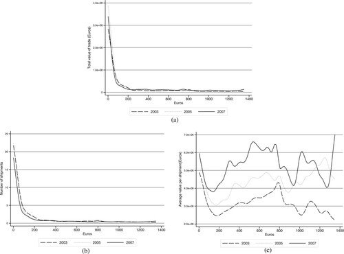
We now resort to non-parametric estimation (kernel regressions) to study spatial trade distribution using the GTC. Figure 2 presents the kernel regressions for each component in equation (1), respectively.⁵ Total value of trade – marginally lower in 2003 than in 2007 as a result of the Spanish economic boom – falls sharply in density as transport costs increase (Figure 2a). This pattern is driven by the number of shipments (extensive margin) (Figure 2b) dropping rapidly for all years up to the point in which an approximate GTC value is reached. The average value per shipment (intensive margin) (Figure 2c), on the other hand, shows an upward trend even with increasing transport costs. This pattern is associated with the price component of the trade flows (see Figure A1 in the supplemental data online) as we discuss below in the fourth section.

Figure 2. Kernel regressions of trade variables on generalized transport costs (GTCs) for pair of municipalities.

ECONOMETRIC SPECIFICATION: TRADE FRICTIONS

In this section we first explore the effects of trade frictions on the total value of trade and its margins in a standard gravity model using the PPML estimator.⁶ We propose a set of regressions in equation (3) for ij municipal pairs (NUTS-5) relying on the trade decompositions presented in equation (1). We include trade flows ($T_{ijt}$) and their margins ($N_{ijt}$, ${\overline{PQ}}_{ijt}$) in levels. Moreover, transport costs are in levels and take a quadratic functional form ($GT{C}_{ijt}$ and $GTCS{q}_{ijt}$) to capture non-linear effects of transport costs on trade flows (Combes et al., 2005) as well as increasing returns to scale in transportation activities (i.e., size of the cargo being transported), coupled with increasing returns to distance as larger batches require larger vehicles (McCann, 2001, 2005). To accurately isolate the effect of municipal border, the contiguity variable is calculated as a first-order queen contiguity that takes the value of 1 when i and j share a border, but also when flows take place within the same municipality (Hillberry, 2002b).

For internal administrative boundaries, we consider three dummy border variables, which are codified as follows: NUTS-5 (municipalities) is set to 1 when flows are performed within the same municipality, and to 0 otherwise; NUTS-3 (provinces) takes the value of 1 when flows are in the same province, but not in the same municipality; and NUTS-2 (regions) captures flows between two municipalities that are located in different provinces but in the same NUTS-2 region. Finally, time, origin and destination fixed effects are included.⁷ Thus, the final specification to estimate takes the form: (3) $\begin{array}{rl}{X}_{ijt}& =\exp [{\text{β}}_0+{\text{β}}_{1}GT{C}_{ijt}+{\text{β}}_{2}GTCS{q}_{ijt}\\ & +{\text{β}}_{3}Contiguit{y}_{ijt}+{\text{β}}_{4}NUTS-5_{ijt}+{\text{β}}_{5}NUTS-3_{ijt}\\ & +{\text{β}}_{6}NUTS-2_{ijt}+yea{r}_t+{\eta }_i+{\eta }_j]\times {ϵ}_{ijt},\end{array}$(3) where $X_{ijt}$ summarizes the trade flows ($T_{ijt}$) and their margins ($N_{ijt}$, $\overline{P{Q}_{ijt}}$). Table 3 shows the results. GTC coefficients exhibit the expected negative sign in the linear component and signal negligible increasing returns in transport (i.e., an infinitesimally positive and significant value in the quadratic term). For internal borders, trade within the same municipality (NUTS-5) is much greater than inter-municipal trade flows. Indeed, the extensive margin achieves a higher NUTS-5 coefficient than the intensive one, indicating that the extensive margin is what truly drives intra-municipal trade flows on average. Other administrative levels (NUTS-3 and NUTS-2) reduce their importance, especially regional flows. It turns out that border effects for relatively long-distance flows between regions are quite reduced or almost negligible, reinforcing the role of local markets and the extensive margin in trade concentrations over short distances. Finally, our results for the border coefficients and $R^2$ get correspondingly better statistical significance and goodness-of-fit than those previously obtained in the literature (Hillberry & Hummels, 2008). Given the number of properties satisfied by the PPML estimators over their ordinary least squares (OLS) counterparts, we are able to accurately capture and explain the trade patterns over very short distances. Indeed, the use of granular measures for trade flows and transport costs reduces the impact of higher regional borders, showing the relevance of the municipal border. That is, these estimations confirm the ‘illusory effect’ of regional borders once lower administrative limits are controlled for. Moreover, they indicate a non-disruption of the market for large administrative levels, in contrast to other studies for Spain (Garmendia et al., 2012; Requena & Llano, 2010) and China (Poncet, 2005).⁸

Table 3. Poisson pseudo-maximum likelihood (PPML) estimations with generalized transport cost (GTC) and internal borders.

Variables	Total value of trade	Extensive margin	Intensive margin
	($T_{ij}$)	($N_{ij}$)	(${\overline{PQ}}_{ij}$)
$GT{C}_{ijt}$	−0.266***	−0.290***	−0.0423***
	(0.0322)	(0.0142)	(0.00537)
$GTCS{q}_{ijt}$	0.000***	0.000***	0.000***
	(0.000)	(0.000)	(0.000)
$Contiguit{y}_{ijt}$	1.365***	1.126***	0.458***
	(0.0708)	(0.0330)	(0.0311)
$NUTS-5_{ijt}$	3.764***	3.236***	0.983***
	(0.101)	(0.0496)	(0.0594)
$NUTS-3_{ijt}$	1.717***	1.406***	0.320***
	(0.0840)	(0.0392)	(0.0255)
$NUTS-2_{ijt}$	0.346***	0.338***	0.0375
	(0.0777)	(0.0354)	(0.0259)
Year FE	Yes	Yes	Yes
Origin FE	Yes	Yes	Yes
Destination FE	Yes	Yes	Yes
N	195,026	195,026	195,026
Pseudo-R^2	0.501	0.772	0.007

Note: Clustered standard errors are by ij. Standard errors are shown in parentheses.

Significance level: ***p < 0.01; **p < 0.05; and *p < 0.1.

FE, fixed effects.

Moving forward, we also study trade dynamics in our panel database. We re-estimate equation (3) in a cross-sectional analysis for 2003 and 2007 independently. Focusing on the relevant results, Table 4 reports only the coefficients for administrative borders. All administrative levels reflect the same pattern for total trade and its margins, that is, there exists a decreasing trend between 2003 and 2007.⁹ Note that the NUTS-5 border in 2003 becomes even larger than in the panel data regressions, whereas the almost null (non-significant) impediments to trade of the NUTS-2 border are confirmed. These findings reflect the time-varying behaviour of the internal home-bias effect, that is, internal borders do not constantly hamper the same amount of trade. Contrary to previous evidence for the US case (Martínez-San Román et al., 2017), Spain experienced a decreasing internal border effect leading to a more trade integration at least in the period 2003–07.

Table 4. Cross-section regressions for 2003 and 2007.

	Border	2003	2007
Total value of trade ($T_{ij}$)	NUTS-5	3.795***	2.835***
	NUTS-3	1.581***	1.079***
	NUTS-2	0.179*	−0.0313
Extensive margin ($N_{ij}$)	NUTS-5	3.151***	2.555***
	NUTS-3	1.184***	0.906***
	NUTS-2	0.174*	−0.00365
Intensive margin (${\overline{PQ}}_{ij}$)	NUTS-5	0.958***	0.841***
	NUTS-3	0.363***	0.291***
	NUTS-2	0.00161	0.0201

Note: Significance level: ***p < 0.01; **p < 0.05; and *p < 0.1.

STRUCTURAL TRADE PATTERNS: GTC THRESHOLDS AND THE GRAVITY MODEL

Breakpoints in the trade flows-to-transport cost relationship

Previous regressions provide an estimate of the internal border effect qualified by the non-linear effect of transport costs and its customary quadratic second-order effect. Nevertheless, this specification does not consider the possibility of having alternative trade frictions once we control for structural changing patterns in trade flows. Visual inspection of the kernel regressions in Figure 2 reveals at least two different trade flows–transport cost structures around a critical value in the interval €110–190, where their non-linear nature is clearly visible. This value implies that in very short distances trade flows are extremely sensitive to relatively low transport costs, particularly in their extensive margin, whereas they are almost independent (‘becoming flat’) for larger GTCs. Indeed, for GTC values larger than the previous range, further and multiple GTC thresholds may coexist at different levels. That is, we should consider and assess the existence of multiple GTC values at which trade flows (structurally) change once they reach one (or several) transport cost thresholds or breakpoints.

As remarked by Abbate et al. (2012), previous studies (Anderson & Yotov, 2012; Eaton & Kortum, 2002; Gallego & Llano, 2014) propose different distance intervals to determine the magnitude of trade barriers, although they arbitrarily define these intervals. On the contrary, we rely on statistical methods to identify these intervals endogenously. We follow Berthelemy and Varoudakis (1996) and apply successive F-tests on stability (Chow tests) that allow us to assess the existence of structural breakpoints in the trade-to-transport cost relationship. Thanks to these non-arbitrary breakpoints we split our transport cost variable into thresholds of distance (GTCs) that can be later considered in our gravity specification in equation (3).

More specifically, we perform a series of Chow tests to check the stability of the relationship between our two variables of interest, trade flows and transport costs. In this context, the Chow test works as follows. First, it divides the sample of trade flows and transport costs (GTC) into two j subsamples, j = 1 and 2, of size $n_j$. Second, it defines a quasi-log-likelihood function such as QL = $-{\sum }_{j=1}^2{n}_j\mathrm{l}\mathrm{n}\left({\sigma }_j^2\right)$. The (Chow) F-stability test detects a GTC breakpoint (valued in monetary terms, €) when the QL function is maximized for two subsamples. In this specific breakpoint, the F-test rejects the null hypothesis (at the 1% and 5% significance levels) of structural stability between trade flows and transport costs.

Note that the Chow test is performed using our specification in equation (3) in which the trade flows are the dependent variable, whereas transport costs (GTC) constitute the threshold variable upon which the breakpoints are detected. Once the first GTC breakpoint is detected using the Chow test, we perform a second test for the subsamples below and above the first GTC breakpoint previously detected. We follow the same logic for the additional subsamples that emerge as further GTC breakpoints appear. Hence, successive Chow tests are applied multiple times in sequential order to check for the existence of successive thresholds.¹⁰ In what follows, sorting the GTC breakpoints from the smallest to the greatest value we obtain the different thresholds defining the extension of successive market areas.

To simplify our stability analysis, we apply this Chow test taking means of our variables in the period 2003–07. This way, we get a cross-sectional version of our panel database.¹¹ As stated, the econometric specification in equation (3) represents our baseline model. Nevertheless, we do not include the quadratic term of the GTC as we aim to determine non-linear relationships by means of transport cost breakpoints. Therefore, including the quadratic term of GTC would distort our analysis on the stability between trade and transports costs.

Table 5 shows the GTC breakpoints obtained for the total value of trade and the extensive margin. Unsurprisingly, the test fails to detect breakpoints for the intensive margin as its components do not drive reductions in trade as shown in the kernel regressions (Figure 2c). However, we confirm the existence of multiple GTC thresholds across the full spectrum of distances, providing strong evidence that trade flows are driven by the extensive margin, especially for short and medium GTCs – the first and second breakpoints for the total value of trade go hand in hand with those from the extensive margin. Moreover, trade flows are highly concentrated at low transport cost values (around €189 and €233), but over longer distances the difference between breakpoints becomes larger, indicating a decline in transport costs as an impediment to trade flows.

Table 5. Generalized transport cost (GTC) breakpoints for the total value of trade and extensive margin: averages for the period 2003–07.

Variable	GTC breakpoints (€)
	Breakpoint 1	Breakpoint 2	Breakpoint 3	Breakpoint 4	Breakpoint 5
$T_{ij}$	189***	233***	285***	513*	706***
$N_{ij}$	185***	246***	321***	582***	655**

Note: Significance level: ***p < 0.01; **p < 0.05; and *p < 0.3.

Figure 3 shows geographical evidence of the existence of these breakpoints by mapping the specific GTC values obtained for the two largest Spanish municipalities: Barcelona and Madrid.¹² The Arc/GIS Network Toolbox allows us to calculate the exact coordinates corresponding to the maximum GTC distance for the type of road and its specific attributes (capacity, gradient, congestion, etc.). Each GTC breakpoint defines an isocost ring whose shape varies with the accessibility of the road network. We refer to the market area comprised within these market isocost rings as natural trade areas because they are defined in monetary transport costs by resorting to the statistical features underlying the Chow structural test.

Figure 3. Natural trade areas using generalized transport cost (GTC) breakpoints.

Note: Averages for the period 2003–07.

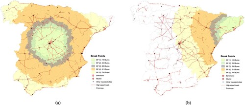
These maps provide a representation of the existence of an urban hierarchical system in terms of trade areas. From these maps several aspects emerge: (1) the first breakpoint refers to the supply centre between the main city and its metropolitan area and other nearby satellite cities; (2) the second and third breakpoints successively reach some important cities (provincial capitals); (3) the fourth breakpoint appears as very relevant because it joins Madrid and Barcelona with other Spanish cities that are wealthy in terms of income and trade (mainly Valencia and Zaragoza); and (4) the last breakpoint directly links Madrid and Barcelona, indicating that trade flows overlap for the two largest Spanish cities. Also, we observe that Barcelona and Madrid have stronger links to other cities densely surrounded by highways. This is the case especially with Madrid, whose road network-centrality allows for larger trade areas reaching all regions in Spain. Finally, note that the geographical extension of the first breakpoint spans over municipal (NUTS-5) and provincial (NUTS-3) borders. It confirms that using administrative boundaries to collect and infer internal border effects could be misleading in its conclusions.

With these findings we argue that the methodology based on the Chow structural and stability test is a promising procedure to determine trade areas, once a correct definition of the dependent and explanatory variables is made available to the analysis. To our knowledge, there is no previous empirical representation of cities’ market areas based on actual trade flows and monetary transport costs (Löffler, 1998). More interestingly, we show in the fifth section that these empirical regularities are in line with the predictions of Lösch and Christaller’s model, whose analytical framework constitutes the core of CPT and gives rise to so-called urban hierarchical systems.

Accounting for GTC thresholds in the gravity model

Once the breakpoints capturing structural changes in the trade-to-transport cost relationship are obtained, we split our GTC distance variable into these GTC thresholds. We perform a set of independent PPML regressions for each GTC threshold using the specification in equation (3), while dropping from each GTC interval the administrative borders in which no observations are recorded. For instance, the transport cost interval of €285–513 (between breakpoints 3 and 4) has no trade flows either at the intra-municipal level or between contiguous municipalities and, therefore, these variables are dropped in the regressions for this interval. We follow the same rationale for the rest of the transport costs intervals. In fact, we contend that this is the correct approach to capture the effects of transport costs and administrative borders in such highly granular trade flows. To give support to this argument, we again perform a general specification using equation (3) and controlling for the standard quadratic non-linear GTC instead of the distance-thresholds approach. As we show in what follows, when using this continuous approach administrative borders overestimate the border effect over short distances.

Tables 6 and 7 show the PPML regression for the total value of trade and the extensive margin for each independent GTCs threshold. For the total value of trade, the GTC is highly penalizing over short distances, but its negative impact decreases as the transport costs increase. It confirms that, first, the negative linear effect of frictions on trade flows varies over the spectrum of distances, and, second, it indicates that transport costs are not as detrimental to trade as normally thought – a result related to the existence of economies of distance and scale on transportation (McCann, 2001). Total trade flows even show a weak positive relationship with transport costs in the range €189–285. This particular result illustrates that total trade is partially driven by the intensive margin (Figure 2c) and, despite growing GTCs, may present steep increases in the value of this margin. It is consistent with the existence of substitution effects in favour of higher price goods (Alchian & Allen, 1964; Hummels & Skiba, 2014), which also corresponds to higher mean price levels dominating the total value of trade (see equation A2 and Figure A1c in the supplemental data online). This result sheds light on some specific features of the trade–transport cost relationship that remain normally unexplored in the literature.

Table 6. Pseudo-maximum likelihood (PPML) estimations by generalized transport cost (GTC) thresholds: total value of trade, averages for the period 2003–07.

	GTC thresholds
${\overline{T}}_{ij}$	(€0–189]	(€189–285]	(€285–513]	(€513–706]	> €706	General specification
${\overline{GTC}}_{ij}$	−0.0145***	0.00262**	−0.00243***	−0.00329***	−0.00142***	−0.00525***
	(0.000339)	(0.00127)	(0.000185)	(0.000309)	(0.000125)	(0.000339)
$\overline{GTC}S{q}_{ij}$	–	–	–	–	–	0.000***
						(0.000)
$Contiguit{y}_{ij}$	0.911***	–	–	–	–	1.232***
	(0.0335)					(0.0702)
$NUTS-5_{ij}$	3.022***	–	–	–	–	3.269***
	(0.0421)					(0.0836)
$NUTS-3_{ij}$	1.059***	2.233***	–	–	–	1.247***
	(0.0348)	(0.318)				(0.0645)
$NUTS-2_{ij}$	0.427***	0.0184	0.189***	1.347***	–	0.0945
	(0.0374)	(0.117)	(0.0708)	(0.102)		(0.0692)
FE origin	Yes	Yes	Yes	Yes	Yes	Yes
FE destiny	Yes	Yes	Yes	Yes	Yes	Yes
N	17,532	4493	7914	4720	4386	39,045
$pseudo-R^2$	0.915	0.546	0.455	0.680	0.407	0.881

Note: Clustered standard errors are by ij. Standard errors are shown in parentheses. Significance level: ***p < 0.01; **p < 0.05; and *p < 0.1.

The use of origin and destiny fixed effects and the lower number of observations in the €189–233 GTC interval forces us to include breakpoint 2 (€233) within the interval €189–285.

FE, fixed effects.

Table 7. Pseudo-maximum likelihood (PPML) estimations by generalized transport cost (GTC) thresholds: extensive margin, averages for the period 2003–07.

	GTC thresholds
${\overline{N}}_{ij}$	(€0–185]	(€185–246]	(€246–321]	(€321–582]	(€582–655]	> €655	General specification
${\overline{GTC}}_{ij}$	−0.0140***	−0.00357***	−0.00528***	−0.00175***	−0.00231***	−0.00133***	−0.00725***
	(0.000199)	(0.000572)	(0.000558)	(0.000143)	(0.000858)	(7.74e–05)	(0.000233)
$\overline{GTC}S{q}_{ij}$	–	–	–	–	–	–	0.000***
							(0.000)
$Contiguit{y}_{ij}$	0.767***	–	–	–	–	–	1.037***
	(0.0171)						(0.0359)
$NUTS-5_{ij}$	2.556***	–	–	–	–	–	2.870***
	(0.0232)						(0.0518)
$NUTS-3_{ij}$	0.808***	1.276***	1.553***	–	–	–	1.060***
	(0.0198)	(0.0789)	(0.101)				(0.0436)
$NUTS-2_{ij}$	0.293***	−0.0164	0.161***	0.553***	–	–	0.118***
	(0.0231)	(0.0363)	(0.0487)	(0.0578)			(0.0423)
Origin FE	Yes	Yes	Yes	Yes	Yes	Yes	Yes
Destiny FE	Yes	Yes	Yes	Yes	Yes	Yes	Yes
N	17,316	3172	2860	8607	1834	5256	39,045
$pseudo-R^2$	0.919	0.774	0.654	0.375	0.802	0.541	0.894

Note: Clustered standard errors are by ij. Standard errors are shown in parentheses. Significance level: ***p < 0.01; **p < 0.05; and *p < 0.1.

FE, fixed effects.

The impact of internal borders is very negative for the total value of trade and its extensive margin before the first threshold is reached, especially the (municipal) NUTS-5 border as in Table 3. NUTS-3 and NUTS-2 again reduce their negative impact as GTC increases, except for the €513–706 GTC interval (€582–655 for the extensive margin), where the regional border has its highest impact on trade flows as a result of being the only border within the interval (extensive margin). Finally, the coefficients for trade frictions in the ‘general specification’ are greater than those obtained for each GTC threshold. Therefore, we conclude that gravity models without transport cost-thresholds do not properly capture, or even overestimate, the impact of transport costs and internal borders.

EXTENSIVE MARGIN, TRADE AREAS AND THE HIERARCHICAL SYSTEM OF CITIES

The GTC breakpoints and the accumulation of trade flows driven by the extensive margin give rise to a series of empirical regularities matching the theoretical insights of CPT and its associated urban hierarchies à la Christaller. Reciprocally, trade in the intensive margin, whose density remains constant as transport costs increase (Figure 2c), reflects persistent trade interactions between high-ranked cities, belonging to the spatial network of locations existing in Spain. The study of these horizontal interactions has been termed as Central Flow Theory (CFT) (Taylor & Derudder, 2016; Zhu et al., 2021) and complements CPT. Whereas the latter focuses on local relationships within the enclosed limits of precise market areas (i.e., the urban centre and its hinterlands), CFT emphasizes the network relationships between high-ranking cities. Both fields of research are experiencing a revival thanks to a new series of studies (Hsu, 2012; Hsu et al., 2014; Mulligan et al., 2012; Parr, 2002; Tabuchi & Thisse, 2011; Taylor & Hoyler, 2021).

Based on CPT, one expects market areas of influence whose geographical reach is driven by transport costs, that is, consumers and firms locate in places where they can be supplied by different cities, and taking into account the transport costs in which they incur because of their consumption or production processes. As a reflection of Von Thünen’s land–rent model, the trade-off between scale economies and transportation costs leads to the emergence of central places, which demand low value-added and homogeneous (standardized) goods from surrounding locations within its market area, while supplying them with a variety of more sophisticated goods. In these models, cities serve those locations for which consumers are willing to cover the transports costs of having the goods shipped to them. Within a given market area, CPT predicts the cooperation between vertically ranked cities located within the same market areas. However, for high-ranked cities, their demand schedules result in larger market areas that, while exhibiting a decreasing density of trade as transport costs increase, come eventually into spatial competition with other cities, that is, their respective market areas overlap (Taylor, 2012).

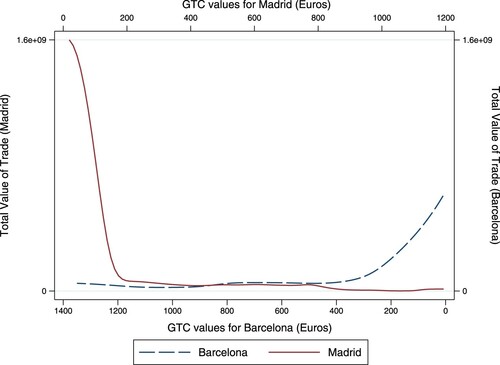
This prediction by CFT across high-ranked cities is shown in our data for Madrid and Barcelona (Figure 3). Using our trade database, we compare in Figure 4 the kernel distributions of trade by distance for the two largest Spanish cities. It is clear that there exists spatial competition between both cities, although they present interesting differences in their trade patterns. While Barcelona spreads along the geography, that is, it presents a larger trade area, Madrid shows a higher density of trade in short distances. That is because the metropolitan area of both cities leads them to supply the surrounding cities in different ways. To meet intermediate production processes and final demand, Madrid has to reach nearby large cities with a high volume of trade by road, while Barcelona uses its port as a supplying hub for its surrounding cities.

Figure 4. Kernel regressions between total value of trade and generalized transport costs (GTCs) for the municipalities of Madrid and Barcelona.

In a stylized version of the CPT model, these cities’ market areas are spatially represented by a lattice of nested hexagons whose radii of influence are determined by the geographical extension of trade flows, which are decreasing in the GTC. Therefore, it is the trade-to-transport cost relationship evidenced through the Chow test and its associated breakpoints that determines, for different cities, the geographical extension of their market areas. In turn, this implies that cities exhibiting high trade densities across longer distances will rank at the upper echelons of the settlement hierarchy, shipping a large range of goods to many commercial partners (corresponding to the extensive margin), and presenting larger GTC thresholds, whereas small cities trade few goods with a small number of cities. Specifically, an urban hierarchy à la Christaller emerges because when considering a range of different goods, few cities can serve high-order items (specialized goods) over long distances, exhibiting longer GTCs thresholds. Meanwhile, as the order-scale of items reduces (low-order items), smaller cities provide more standardized products. In this sense:

the most central location in the entire system provides all of its goods and services thereby satisfying the so called exhaustive principle. But, moving down through this functional continuum (of goods), other locations on the landscape are sufficiently well located to provide some, but not all, goods that are provided at the most central location.

(Mulligan et al., 2012, p. 404)

That is, in the hierarchy of cities represented by the CPT, we should expect one or few cities (rank 1) to harbour the largest market areas and supply a full range of products, a second group of large cities (rank 2) to serve a huge variety of commodities within a still relatively large market area, and a lower tier of medium and small-size cities (ranks 3 and 4) to be geographically scattered across the space and trading fewer products with smaller or even insignificant market areas (Tabuchi & Thisse, 2011). Since the density of trade flows highly correlates with the number of varieties (goods) being traded and the number of trading partners, we rely on these data to perform a cluster analysis that classifies cities into ranking positions depending on the values of these two variables. This approach concurs with the assumptions of CPT and can be traced back to Christaller himself (Preston, 2009; Taylor & Hoyler, 2021; Zhu et al., 2021).

Empirical studies testing urban hierarchy systems based on CPT have focused only on urban population patterns and administrative borders, even when theoretical predictions and the underlying assumptions relate it to the magnitude and composition of trade flows. The reason to rely on the population proxy for trade flows is the scarcity of intercity trade data. The underlying assumption is that population size is not only a good proxy of a city market area, but also implies a more diversified demand that supports the production of a wider range of products. Thanks to our highly granular trade flows, we can now test these predictions following the aforementioned approach that relies on actual trade data. Table 8 decomposes the extensive margin of trade and shows the distributions of the Spanish municipalities in 2003 and 2007 according to the number of different commodities traded by each municipality and the number of municipalities (trading partners) with which trade takes place, that is, $N_{ij}^k$, as defined in equation A1 and Figure A1a in the supplemental data online. Data are expressed as a percentage over the total number of municipalities. As observed, the largest number of municipalities trade between 10 and 50 commodities (10 $<k\le$ 50) with a set of 10–50 municipalities (10 $<j\le$ 50). The same follows for intervals greater than 50 commodities and 50 municipalities. More interestingly, these results shed light on a hierarchy of cities. The main diagonal characterizes various municipalities: a vast majority of them trade few commodities with few trading partners (these municipalities are subsequently classified as rank 4 and 3 locations by our cluster analysis), another group of municipalities trades an increasing number commodities with more municipalities (rank 2), and finally a group of only few municipalities trade a huge number of commodities (more than 100) with a large number partners (more than 100) (rank 1).

Table 8. Distribution of municipalities by different products and trading partners: $N_{ij}^k$. Percentage of municipalities in each interval, 2003 and 2007.

	Number of trading partners
Number of commodities	(1–10]	(10–50]	(50–100]	>100
2003
(1–10]	3.04%	8.61%	0.16%	0.00%
(10–50]	0.32%	38.6%	11.0%	0.16%
(50–100]	0.00%	1.91%	17.3%	2.71%
> 100	0.00%	0.00%	1.91%	14.19%
2007
(1–10]	1.92%	5.43%	0.00%	0.00%
(10–50]	1.12%	42.1%	8.31%	0.00%
(50–100]	0.00%	1.76%	19.1%	1.60%
> 100	0.00%	0.00%	3.04%	15.5%

Source: Authors’ own elaboration from the Spanish Road Freight Transportation Survey (RFTS) data.

Table 8 sheds light on the urban hierarchy system. As it can be observed, the main diagonal characterizes different types of cities in the lines expressed above. We rely on cluster analysis to group these municipalities getting further evidence of the hierarchy of cities.¹³ The group classification of cities obtained with the cluster analysis is reported in Table 9, with an overwhelming predominance of medium and small municipalities (ranks 3 and 4) and a skewness distribution for the largest ones (ranks 1 and 2).

Table 9. Municipalities grouped by clusters: averages for the period 2003–07.

Municipal rank	Number of municipalities
Rank 1	4
Rank 2	21
Rank 3	101
Rank 4	507

Figure 5 confirms the theoretical insights of CPT by means of kernel regressions for each group of clustered municipalities. Those belonging to a higher rank present higher trade densities across all distances (GTCs), especially over short ones. Moreover, the elasticity of shipments to GTCs is lower for all transport costs, that is, in the short distances ranks 3 and 4 cities are not as sensitive to GTCs as higher ranked cities. The overall concentration of trade flows in short distances observed in Figure 2 is clearly driven by these ranks 1 and 2 municipalities whose higher kernels envelop those of lower ranks.

Figure 5. Kernel regressions between total trade and generalized transport costs (GTCs) for each pair of municipalities grouping them by clusters.

Note: Averages for the period 2003–07.

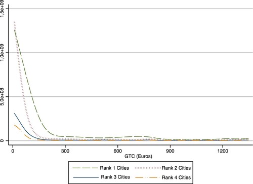
Furthermore, Table 10 presents the results of applying the Chow test methodology to each of these four city ranks. We report the identified breakpoints ($GT{C}_{ij}$ in €), along with the average value of trade observed at each breakpoint ($T_{ij}$), and the value of trade per euro of transport cost ($T_{ij}/GT{C}_{ij}$). The results clearly show that higher ranked cities present larger market areas by trading more for any given GTC threshold or, equivalently, that a given value of trade is achieved at lower GTCs for higher ranked cities. Note that the method identifies a single breakpoint for rank 4 cities because their trade values over short distances are much lower.

Table 10. Generalized transport cost (GTC) breakpoints by city rank: averages for the period 2003–07.

City	Variable	Breakpoint 1	Breakpoint 2	Breakpoint 3	Breakpoint 4
Rank 1	$GT{C}_{ij}$ (€)	94***	188***	261***	665***
	$T_{ij}$ (logs)	17.73	16.33	16.28	16.21
	$T_{ij}$/$GT{C}_{ij}$ (logs)	13.18	11.07	10.71	9.71
Rank 2	$GT{C}_{ij}$ (€)	144***	262***	609***	676***
	$T_{ij}$ (logs)	15.67	14.95	15.31	15.18
	$T_{ij}$/$GT{C}_{ij}$ (logs)	10.72	9.38	8.90	8.67
Rank 3	$GT{C}_{ij}$ (€)	277***	430***	681***	756***
	$T_{ij}$ (logs)	14.32	14.61	14.78	15.12
	$T_{ij}$/$GT{C}_{ij}$ (logs)	8.69	8.55	8.26	8.49
Rank 4	$GT{C}_{ij}$ (€)	257***	–	–	–
	$T_{ij}$ (logs)	14.05
	$T_{ij}$/$GT{C}_{ij}$ (logs)	8.50

Note: Significance level: ***p < 0.01; **p < 0.05; and *p < 0.1.

We map the Spanish urban hierarchy from these results. To our knowledge, Figure 6 is the first illustration of a hierarchy based on trade flows, differentiating municipalities by their rank. We show the market areas corresponding to the breakpoints reported in Table 10 for rank 1 municipalities (Madrid, Barcelona, Valencia and Seville). The first threshold (BP(1):€94), covers their metropolitan areas, whereas their second and third breakpoints reach rank 2 or even rank 3 municipalities, as predicted by CPT. There is an additional breakpoint at the value of €665 that we do not show to ease the readability of the map This last breakpoint represents the distance between the rank 1 cities, particularly Madrid and Barcelona, emphasizing the results illustrated in Figure 4.

Figure 6. Urban hierarchy and natural trade areas for rank 1 municipalities.

Note: Plotted are the first, second and third generalized transport cost (GTC) breakpoints. The fourth breakpoint is equal to e665.

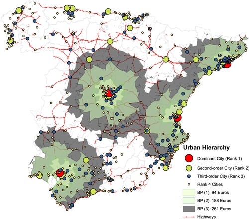
Moreover, taking as reference Figure 6, if we portrayed the rings corresponding to the market areas of lower ranked cities based on the density of trade values by GTC thresholds, this would show that their (smaller) market areas are nested (or ‘enveloped’) within the (larger) market areas of higher ranked cities. For instance, the second breakpoint for rank 1 cities, equal to €188, and presenting an average value of trade of 16.33 (in logs), is greater than the first breakpoint for rank 2 cities, €144, whose value of trade is smaller at 15.67 (in logs). This relationship holds as we move towards higher breakpoints and city ranks. In this regard, Figure 6 resembles the classical lattice of nested hexagons represented in Christaller’s diagram. Nevertheless, we recall that Christaller’s model constitutes a stylized representation of precise geometrical relationships and, therefore, the actual size of real market areas may not match exactly the patterns of a hexagon lattice. First, markets areas may overlap, that is, following Taylor (2012) cities compete for commercial influence, as shown above for Madrid and Barcelona. Second, low ranked market areas may fall within two high-ranked market areas, a situation that in Christaller’s idealized model does not occur. Third, it is also worth noticing that the geographical extension of the detected breakpoints exceeds internal administrative borders, particularly NUTS-5 (municipal) and NUTS-3 (provincial) territorial units, that is, trading activity spans several administrative levels. Overall, in light of these results, we contend that the high agglomeration of trade flows at the municipal level obtained in Table 3 is mostly driven by the trading activity of ranks 1 and 2 cities.

CONCLUSIONS

We compiled two unique and granular databases of municipal trade flows and monetary transport costs to assess trade agglomerations around specific areas (municipalities). Relying on the gravity model, we focus on the role played by trade frictions and intra-national borders to show that regional borders have a much lower or even negligible impact on trade, whereas NUTS-5 borders and surrounding areas concentrate the largest share of trade flows. In contrast to previous studies, we argue that this trade agglomeration over short distances has nothing to do with (unreal) border impediments, but arises as a result of transport cost thresholds that shape trade market areas around large municipalities, thereby defining a hierarchical system of cities.

To confirm this idea, we apply the endogenous Chow test to the trade literature, allowing us to determine these specific breakpoints at which trade flows change structurally with transport costs. With this approach, we correctly measure the impact of internal borders and confirm the high density of trade at GTC values below €189 (equivalent to approximately 170 km or 110 min). Finally, we map these GTC breakpoints showing the emergence of an organized system of cities in terms of trade market areas in which trade agglomerations are driven by the largest municipalities in the urban hierarchy. We highlight that these results provide empirical evidence for the insights of the CPT and call for future research on the spatial trade distribution of the Spanish cities.

DISCLOSURE STATEMENT

No potential conflict of interest was reported by the authors.

Additional information

Funding

This work was supported by MINECO [grant number ECO2013-46980-P]; and the Ministerio de Educacion, Cultura y Deporte [grant number FPU-2010].

Notes

1. Although the lack of official databases on intra-national trade flows discourages empirical trade analysis, recent and prominent studies provide estimates that apply context-specific techniques to survey data (Wolf, 2000; Hillberry, 2002a; Hillberry & Hummels, 2008), use other official data sources at the national level (Poncet, 2005; Yilmazkuday, 2011, 2012) or rely on regional input–output databases (Thissen et al., 2019).

2. For a full description of the elaboration of the trade database, see Appendix A1 in the supplemental data online.

3. Appendix A2 in the supplemental data online explores a second-level decomposition for the extensive and intensive margins.

4. For a complete presentation of GTC methods, their calculation over time in real terms and the definition of suitable variation indices, see Zofío et al. (2014) for the Spanish case and Persyn et al. (2020) for the whole European Union region.

5. We use the Gaussian kernel estimator with n=100 points and allow it to calculate and employ the optimal bandwidth.

6. The PPML method accounts for the fact that the sample of municipalities includes a large number of zeros, offering estimators that are more efficient than their OLS counterparts. This method identifies and eventually drops regressors that may cause the non-existence of (pseudo-) maximum likelihood estimates. Therefore, it presents several advantages for trade data in light of the problems posed by the presence of numerous zeros, and in the presence of dummies (see also Head & Mayer, 2014). In addition, the PPML can resolve the bias caused by heteroscedasticity, serial correlated error and multicollinearity due to a high correlation among determinants in the gravity equation and the origin–destination fixed effects.

7. We control for time, origin and destination fixed effects to recover estimates on time-invariant controls, although our estimates remain robust to the inclusion of origin–year and destination–year fixed effects. We acknowledge that further developments of the PPML estimator allow us to include time-invariant dyadic fixed effects (Correia et al., 2020), but thanks to the inclusion of our main variable of interest, the bilateral GTC, plus the other dyadic variables (contiguity and administrative borders), we are able to capture bilateral characteristics between all pairs of municipalities.

8. Appendix A3 in the supplemental data online discusses equivalent PPML regressions for the second level of the trade flows decomposition.

9. We perform a set of mean tests and reject the null hypotheses of equal border coefficients between 2003 and 2007.

10. As argued by Diallo (2014), the advantage of this endogenous version of the Chow stability test is that it is not required to provide in advance a breakpoint at which we suspect the existence of a structural change in the stability between our variables of interests. Instead, it endogenously determines the exact (GTC) breakpoint at which the dependent variable (trade flows) changes structurally with respect to our GTC variable. This test is available in STATA thanks to Diallo (2014) (see also Berthelemy & Varoudakis, 1996, for an application of the Chow test in the economic growth literature).

11. We choose to convert our panel database for the period 2003–07 into a cross-sectional version of it based on averages of our trade and transport costs variables because applying the Chow test for the individual years 2003–07 gives approximately similar GTC breakpoints as those finally reported in Table 5.

12. The GTC values in the maps are the same in as those in Table 5, but expressed in distance-equivalent terms, so as to be able to plot them with Arc/GIS software. The GTCs represented are those obtained for the complete sample of 633 municipalities, but city-specific breakpoints could be also provided by the authors upon request.

13. We base our municipal cluster analysis on the averages for the number of commodities and the number of trading partners for each municipality in the period 2003–07. We use the K-means (centroids) algorithm and obtain the four groups portrayed after 25 iterations.

REFERENCES

- Abbate, A., De Benedictis, L., Fagiolo, G., & Tajoli, L. (2012). The international trade network in space and time (LEM Working Paper Series No. 2012/17).
- Alchian, A., & Allen, W. (1964). University economics. Wadsworth.
- Anas, A., & Xiong, K. (2003). Intercity trade and the industrial diversification of cities. Journal of Urban Economics, 54(2), 258–276. https://doi.org/https://doi.org/10.1016/S0094-1190(03)00073-1
- Anderson, J., & Yotov, Y. (2012). Gold standard gravity (Working Paper No. 17835). National Bureau of Economic Research (NBER).
- Andresen, M. (2010). The geography of the Canada–United States border effect. Regional Studies, 44(5), 579–594. https://doi.org/https://doi.org/10.1080/00343400802508794
- Behrens, K., Mion, G., Murata, Y., & Suedekum, J. (2017). Spatial frictions. Journal of Urban Economics, 97, 40–70. https://doi.org/https://doi.org/10.1016/j.jue.2016.11.003
- Berthelemy, J., & Varoudakis, A. (1996). Economic growth, convergence clubs, and the role of financial development. Oxford Economic Papers, 48(2), 300–328. https://doi.org/https://doi.org/10.1093/oxfordjournals.oep.a028570
- Capello, R., Caragliu, A., & Fratesi, U. (2018a). Breaking down the border: Physical, institutional and cultural obstacles. Economic Geography, 94(5), 485–513. https://doi.org/https://doi.org/10.1080/00130095.2018.1444988
- Capello, R., Caragliu, A., & Fratesi, U. (2018b). Measuring border effects in European cross-border regions. Regional Studies, 52(7), 986–996. https://doi.org/https://doi.org/10.1080/00343404.2017.1364843
- Cavailhes, J., Gaigne, C., Tabuchi, T., & Thisse, J. (2007). Trade and the structure of cities. Journal of Urban Economics, 62(3), 383–404. https://doi.org/https://doi.org/10.1016/j.jue.2006.12.002
- Combes, P., & Lafourcade, M. (2005). Transport costs: Measures, determinants, and regional policy implications for France. Journal of Economic Geography, 5(3), 319–349. https://doi.org/https://doi.org/10.1093/jnlecg/lbh062
- Combes, P., Lafourcade, M., & Mayer, T. (2005). The trade-creating effects of business and social networks: Evidence from France. Journal of International Economics, 66(1), 1–29. https://doi.org/https://doi.org/10.1016/j.jinteco.2004.07.003
- Correia, S., Guimarães, P., & Zylkin, T. (2020). Fast Poisson estimation with high-dimensional fixed effects. The Stata Journal: Promoting Communications on Statistics and Stata, 20(1), 95–115. https://doi.org/https://doi.org/10.1177/1536867X20909691
- Crafts, N., & Klein, A. (2014). Geography and intra-national home bias: US domestic trade in 1949 and 2007. Journal of Economic Geography, 15(3), 477–497. https://doi.org/https://doi.org/10.1093/jeg/lbu008
- Diallo, I. (2014). Suchowtest: Stata module to calculate successive Chow tests on cross section data (Statistical Software Components No. S457536). Boston College Department of Economics.
- Eaton, J., & Kortum, S. (2002). Technology, geography, and trade. Econometrica, 70(5), 1741–1779. https://doi.org/https://doi.org/10.1111/1468-0262.00352
- Gallego, N., & Llano, C. (2014). The border effect and the nonlinear relationship between trade and distance. Review of International Economics, 22(5), 1016–1048. https://doi.org/https://doi.org/10.1111/roie.12152
- Gallego, N., Llano, C., De la Mata, T., & Díaz-Lanchas, J. (2015). Intranational home bias in the presence of wholesalers, hub–spoke structures and multimodal transport deliveries. Spatial Economic Analysis, 10(3), 369–399. https://doi.org/https://doi.org/10.1080/17421772.2015.1062126
- Garmendia, A., Llano, C., Minondo, A., & Requena, F. (2012). Networks and the disappearance of the intranational home bias. Economics Letters, 116(2), 178–182. https://doi.org/https://doi.org/10.1016/j.econlet.2012.02.021
- Head, K., & Mayer, T. (2014). Gravity equations: Workhorse, toolkit and cookbook. Handbook of International Economics, 4, 131–195. https://doi.org/https://doi.org/10.1016/B978-0-444-54314-1.00003-3
- Hillberry, R. (2002a). Aggregation bias, compositional change, and the border effect. Canadian Journal of Economics, 35(3), 517–530. https://doi.org/https://doi.org/10.1111/1540-5982.00143
- Hillberry, R. (2002b). Commodity flow survey data documentation (Technical Report). US International Trade Commission, Forum for Research in Empirical International Trade (FREIT).
- Hillberry, R., & Hummels, D. (2003). Intranational home bias: Some explanations. Review of Economics and Statistics, 85(4), 1089–1092. https://doi.org/https://doi.org/10.1162/003465303772815970
- Hillberry, R., & Hummels, D. (2008). Trade responses to geographic frictions: A decomposition using micro-data. European Economic Review, 52(3), 527–550. https://doi.org/https://doi.org/10.1016/j.euroecorev.2007.03.003
- Hsu, W. (2012). Central place theory and city size distribution. The Economic Journal, 122(563), 903–932. https://doi.org/https://doi.org/10.1111/j.1468-0297.2012.02518.x
- Hsu, W., Holmes, T., & Morgan, F. (2014). Optimal city hierarchy: A dynamic programming approach to central place theory. Journal of Economic Theory, 154, 245–273. https://doi.org/https://doi.org/10.1016/j.jet.2014.09.018
- Hummels, D., & Skiba, A. (2004). Shipping the good apples out? An empirical confirmation of the Alchian–Allen conjecture. Journal of Political Economy, 112(6), 1384–1402. https://doi.org/https://doi.org/10.1086/422562
- Llano, C., De la Mata, T., Díaz-Lanchas, J., & Gallego, N. (2017). Transport-mode competition in intra-national trade: An empirical investigation for the Spanish case. Transportation Research Part A: Policy and Practice, 95, 334–355. https://doi.org/https://doi.org/10.1016/j.tra.2016.10.023
- Llano-Verduras, C., Minondo, A., & Requena-Silvente, F. (2011). Is the border effect an artefact of geographical aggregation? The World Economy, 34(10), 1771–1787. https://doi.org/https://doi.org/10.1111/j.1467-9701.2011.01398.x
- Löffler, G. (1998). Market areas – A methodological reflection on their boundaries. GeoJournal, 45(4), 265–272. https://doi.org/https://doi.org/10.1023/A:1006980420829
- Martínez-San Román, V., Mateo-Mantecón, I., & Sainz-González, R. (2017). Intra-national home bias: New evidence from the United States commodity flow survey. Economics Letters, 151, 4–9. https://doi.org/https://doi.org/10.1016/j.econlet.2016.11.038
- McCann, P. (2001). A proof of the relationship between optimal vehicle size, haulage length, and the structure of transport–distance costs. Transportation Research Part A: Policy and Practice, 35(8), 671–693. https://doi.org/https://doi.org/10.1016/S0965-8564(00)00011-2
- McCann, P. (2005). Transport costs and new economic geography. Journal of Economic Geography, 5(3), 305–318. https://doi.org/https://doi.org/10.1093/jnlecg/lbh050
- Mori, T., & Wrona, J. (2018). Inter-city trade (DICE Discussion Paper No. 298). http://hdl.handle.net/10419/181968.
- Mulligan, G., Partridge, M., & Carruthers, J. (2012). Central place theory and its reemergence in regional science. The Annals of Regional Science, 48(2), 405–431. https://doi.org/https://doi.org/10.1007/s00168-011-0496-7
- Nitsch, V., & Wolf, N. (2013). Tear down this wall: On the persistence of borders in trade. Canadian Journal of Economics, 46(1), 154–179. https://doi.org/https://doi.org/10.1111/caje.12002
- Parr, J. (2002). The location of economic activity: Central place theory and the wider urban system. Edward Elgar.
- Persyn, D., Díaz-Lanchas, J., & Barbero, J. (2020). Estimating road transport costs between EU regions. Transport Policy, forthcoming. https://doi.org/https://doi.org/10.1016/j.tranpol.2020.04.006
- Poncet, S. (2005). A fragmented China: Measure and determinants of Chinese domestic market disintegration. Review of International Economics, 13(3), 409–430. https://doi.org/https://doi.org/10.1111/j.1467-9396.2005.00514.x
- Preston, R. (2009). Walter Christaller’s research on regional and rural development planning during World War I (Papers in Metropolitan Studies No. METAR 52/2009). Freie Universität Berlin.
- Ramos, R., & Moral-Benito, E. (2017). Agglomeration by export destination: Evidence from Spain. Journal of Economic Geography, 18(3), 599–625. https://doi.org/https://doi.org/10.1093/jeg/lbx038
- Requena, F., & Llano, C. (2010). The border effects in Spain: An industry-level analysis. Empirica, 37(4), 455–476. https://doi.org/https://doi.org/10.1007/s10663-010-9123-6
- Santos Silva, J., & Tenreyro, S. (2006). The log of gravity. The Review of Economics and Statistics, 88(4), 641–658. https://doi.org/https://doi.org/10.1162/rest.88.4.641
- Santos Silva, J., & Tenreyro, S. (2010). On the existence of the maximum likelihood estimates in Poisson regression. Economics Letters, 107(2), 310–312. https://doi.org/https://doi.org/10.1016/j.econlet.2010.02.020
- Santos Silva, J., & Tenreyro, S. (2011). Further simulation evidence on the performance of the Poisson pseudo-maximum likelihood estimator. Economics Letters, 112(2), 220–222. https://doi.org/https://doi.org/10.1016/j.econlet.2011.05.008
- Sohn, C., & Licheron, J. (2018). The multiple effects of borders on metropolitan functions in Europe. Regional Studies, 52(11), 1512–1524. https://doi.org/https://doi.org/10.1080/00343404.2017.1410537
- Tabuchi, T., & Thisse, J. (2011). A new economic geography model of central places. Journal of Urban Economics, 69(2), 240–252. https://doi.org/https://doi.org/10.1016/j.jue.2010.11.001
- Taylor, P., & Derudder, B. (2016). World city network: A global urban analysis (2nd ed.). Routledge.
- Taylor, P. J. (2012). On city cooperation and city competition. In B. Derudder, M. Hoyler, P. Taylor, & F. Witlox (Eds.), International handbook of globalization and world cities (pp. 64–72). Edward Elgar.
- Taylor, P. J., & Hoyler, M. (2021). Lost in plain sight: Revealing central flow process in Christaller's original central place systems. Regional Studies, 55(2), 345–353. https://doi.org/10.1080/00343404.2020.1772965
- Thissen, M., Olga, I., Mandras, G., & Husby, T. (2019). European NUTS 2 regions: Construction of interregional trade-linked supply and use tables with consistent transport flows (JRC Working Papers on Territorial Modelling and Analysis No. 2019/01). Joint Research Centre (Seville).
- Tubadji, A., & Nijkamp, P. (2015). Cultural gravity effects among migrants: A comparative analysis of the EU15. Economic Geography, 91(3), 343–380. https://doi.org/https://doi.org/10.1111/ecge.12088
- Wolf, H. (1997). Patterns of intra- and inter-state trade (Working Paper No. 5939). National Bureau of Economic Research (NBER).
- Wolf, H. (2000). Intranational home bias in trade. Review of Economics and Statistics, 82(4), 555–563. https://doi.org/https://doi.org/10.1162/003465300559046
- Wrona, J. (2018). Border effects without borders: What divides Japan’s internal trade? International Economic Review, 59(3), 1209–1262. https://doi.org/https://doi.org/10.1111/iere.12302
- Yi, K. (2010). Can multistage production explain the home bias in trade? American Economic Review, 100(1), 364–393. https://doi.org/https://doi.org/10.1257/aer.100.1.364
- Yilmazkuday, H. (2011). Agglomeration and trade: State-level evidence from U.S. industries. Journal of Regional Science, 51(1), 139–166. https://doi.org/https://doi.org/10.1111/j.1467-9787.2010.00684.x
- Yilmazkuday, H. (2012). Understanding interstate trade patterns. Journal of International Economics, 86(1), 158–166. https://doi.org/https://doi.org/10.1016/j.jinteco.2011.08.015
- Zhu, B., Pain, K., Taylor, P., & Derudder, B. (2021). Exploring external urban relational processes: Inter-city financial flows complementing global city-regions. Regional Studies. https://doi.org/https://doi.org/10.1080/00343404.2021.1921136.
- Zofío, J. L., Condeço-Melhorado, A. M., Maroto-Sánchez, A., & Gutiérrez, J. (2014). Generalized transport costs and index numbers: A geographical analysis of economic and infrastructure fundamentals. Transportation Research Part A: Policy and Practice, 67, 141–157. https://doi.org/https://doi.org/10.1016/j.tra.2014.06.009